Full article: Dynamics of a diffusive vaccination model with therapeutic impact and non-linear incidence in epidemiology

Formulae display: $MathJax Logo$ ?Mathematical formulae have been encoded as MathML and are displayed in this HTML version using MathJax in order to improve their display. Uncheck the box to turn MathJax off. This feature requires Javascript. Click on a formula to zoom.

Abstract

In this paper, we study a more general diffusive spatially dependent vaccination model for infectious disease. In our diffusive vaccination model, we consider both therapeutic impact and nonlinear incidence rate. Also, in this model, the number of compartments of susceptible, vaccinated and infectious individuals are considered to be functions of both time and location, where the set of locations (equivalently, spatial habitats) is a subset of $R^{n}$ with a smooth boundary. Both local and global stability of the model are studied. Our study shows that if the threshold level $R_{0} \leq 1,$ the disease-free equilibrium $E_{0}$ is globally asymptotically stable. On the other hand, if $R_{0} > 1$ then there exists a unique stable disease equilibrium $E^{*}$ . The existence of solutions of the model and uniform persistence results are studied. Finally, using finite difference scheme, we present a number of numerical examples to verify our analytical results. Our results indicate that the global dynamics of the model are completely determined by the threshold value $R_{0}$ .

Keywords:

2010 Mathematics Subject Classifications:

1. Introduction

Mathematical and epidemiological models are important tools for analysing various real world phenomena in health science and epidemiology. For infectious diseases, many mathematical and epidemiological models have been studied by researchers to understand the effect of vaccination for controlling the spread of infectious diseases. Diffusive vaccination models are useful models for analysing the impact of vaccination for infectious diseases. Moreover, diffusive vaccination models are useful for getting information about how to control the reasoning individuals.

It is known that vaccine works with the immune system. Evidently as the disease can not provide immunity, so not the vaccination. As a result, most of the diseases have a recovered/immune stage for which vaccination is successful. Some other bacteria can remain in the host without causing any disease. This scenario is called carriage. The following SIS model, a model where recovery is short lived, that is, brings the individuals return to the susceptible class is considerable in this action with vaccination [Citation22]: $\begin{aligned} \begin{array}{lll} \frac{d S}{d t} = a - b q_{1} I S - (m + n) S, & f o r t \in (0, \infty) w i t h S (0) = S^{0}, \\ \frac{d V}{d t} = n S - b q_{2} I V - m V, & f o r t \in (0, \infty) w i t h V (0) = V^{0}, \\ \frac{d I}{d t} = b q_{1} I S + b q_{2} I V - m I, & f o r t \in (0, \infty) w i t h I (0) = I^{0} . \end{array} \end{aligned}$ where S, V, I are the number of compartments of susceptible individuals, vaccinated individuals and infectious individuals at time t, respectively. 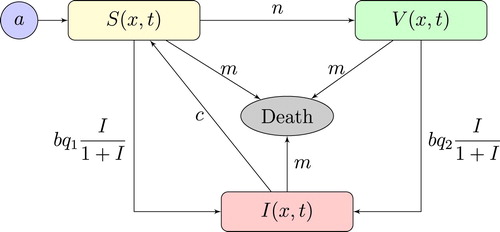a is the recruitment rate of susceptible individuals, $q_{1}$ and $q_{2}$ are the transmission probabilities of susceptible and vaccinated individuals, the parameter b is the average number of contact partners, n is the vaccination coverage of susceptible individuals, m is the natural death. Since the model monitors population dynamics, it follows that all it's dependent variables and parameters must be non-negative. Further, it is assumed that the prevalent disease does not kill infectious individuals, and treatment does not offer permanent immunity.

Periodic fluctuations occurs in many infectious diseases. Such periodic fluctuations may be driven by extrinsic factors, as reflected in periodic transmission rates, e.g. seasonality [Citation4, Citation20, Citation27], or may be caused by time delays [Citation13], age structure [Citation26], or non-linearity of incidence rates [Citation34]. In the above SIS model, the incidence rate is bilinear, and is given by $b q_{1} I S$ . The bilinear model generally admits a trivial equilibrium (I = 0) corresponding to the case in which the disease is not present. It also may admit a stable non-trivial equilibrium corresponding to the situation in which the disease is maintained. Wilson and Worcester [Citation34] were the first to consider the more general incidence rate with a factor $S^{p}$ and their primarily goal was to investigate the consequences of various assumptions when the laws are not known. In 1969, Severo [Citation28] considered a more general bilinear form $k I^{p} S^{q}$ with q<1. Severo [Citation28] also considered a nonlinear recovery rate. Capasso and Serio [Citation7] generalized the incidence rate by considering the bilinear term of the form $k g (I) S$ with the condition $g' (0)$ positive and finite. The model of Capasso and Serio [Citation7] excludes the form $k I^{p} S$ if $p \neq 1.$ Cunningham [Citation33] pointed out that there may exist periodic solutions in a model with an incidence rate $k (I S)^{p}$ with $p > 1.$

In 1986 and 1987 respectively, Liu et. al. [Citation18, Citation19] considered some general incidence rates. They also analysed the conditions under which a Hopf bifurcation occurs for a stable periodic solution and they discussed possible mechanisms for underlying nonlinear incidence rates of the following system $\begin{aligned} \begin{array}{lll} \frac{d S}{d t} = a - b q_{1} H (I) S - (m + n) S, & f o r t \in (0, \infty) w i t h S (0) = S^{0}, \\ \frac{d V}{d t} = n S - b q_{2} H (I) V - m V, & f o r t \in (0, \infty) w i t h V (0) = V^{0}, \\ \frac{d I}{d t} = b q_{1} H (I) S + b q_{2} H (I) V - m I, & f o r t \in (0, \infty) w i t h I (0) = I^{0} . \end{array} \end{aligned}$ The authors also suggested to consider other forms for the incidence rate and the effects of disease-induced mortality.

In recent years, many other mathematical and epidemiological models have been studied by researchers with different types of interesting incidence rates. Gumel and Moghadas [Citation10] studied the following deterministic epidemic model with non-linear incidence $H (I) = \frac{I}{1 + I}$ (1) $\begin{aligned} \begin{array}{lll} \frac{d S}{d t} = a - b q_{1} \frac{I}{1 + I} S - (m + n) S + c I & f o r t \in (0, \infty), w i t h S (0) = S^{0}; \\ \frac{d V}{d t} = n S - b q_{2} \frac{I}{1 + I} V - m V & f o r t \in (0, \infty), w i t h V (0) = V^{0}; \\ \frac{d I}{d t} = b q_{1} \frac{I}{1 + I} S + b q_{2} \frac{I}{1 + I} V - m I - c I & f o r t \in (0, \infty), w i t h I (0) = I^{0} . \end{array} \end{aligned}$ (1) In the above model, the authors introduced the parameter c, the therapeutic treatment coverage of infectious individuals $I (t)$ removed to $S (t)$ compartment. Note that the above model is an SIS model and it was shown that the effectively treated infectious individuals return to the susceptible compartments and behaves similarly. The authors also observed realistically that $q_{2} \leq q_{1}$ from the fact that vaccination can reduce or eliminate the incidence of infection. Also, Gumel and Moghadas [Citation10] analysed the corresponding characteristic equation and studied the local stability of its disease-free and disease equilibria and the optimal vaccine coverage threshold needed for disease control and eradication analytically. In 2014, Buonomo et al. [Citation5] constructed suitable Lyapunov functions and established global stability of disease-free and disease equilibrium of the above system (Equation1(1) $\begin{aligned} \begin{array}{lll} \frac{d S}{d t} = a - b q_{1} \frac{I}{1 + I} S - (m + n) S + c I & f o r t \in (0, \infty), w i t h S (0) = S^{0}; \\ \frac{d V}{d t} = n S - b q_{2} \frac{I}{1 + I} V - m V & f o r t \in (0, \infty), w i t h V (0) = V^{0}; \\ \frac{d I}{d t} = b q_{1} \frac{I}{1 + I} S + b q_{2} \frac{I}{1 + I} V - m I - c I & f o r t \in (0, \infty), w i t h I (0) = I^{0} . \end{array} \end{aligned}$ (1) ) by using LaSalle's invariance principle [Citation16]. The authors also presented optimal vaccination and treatment strategies to minimize both the disease burden and intervention.

Recently, many researchers have considered spatial structure as a central factor because it affects the spatial spreading of disease [Citation1, Citation2, Citation6, Citation14, Citation15, Citation24, Citation38, Citation39]. In this paper, we propose a spatially dependent vaccination model which is a diffusive version of the above model (Equation1(1) $\begin{aligned} \begin{array}{lll} \frac{d S}{d t} = a - b q_{1} \frac{I}{1 + I} S - (m + n) S + c I & f o r t \in (0, \infty), w i t h S (0) = S^{0}; \\ \frac{d V}{d t} = n S - b q_{2} \frac{I}{1 + I} V - m V & f o r t \in (0, \infty), w i t h V (0) = V^{0}; \\ \frac{d I}{d t} = b q_{1} \frac{I}{1 + I} S + b q_{2} \frac{I}{1 + I} V - m I - c I & f o r t \in (0, \infty), w i t h I (0) = I^{0} . \end{array} \end{aligned}$ (1) ), where we consider the individual movements of all three compartment cells. We strongly believe that our proposed model is a more general and realistic biological and epidemiological model. Throughout the paper, we use the following notation for simplicity: $A = Ω \times (0, \infty)$ and $\partial A = \partial Ω \times (0, \infty) .$ In the following, we present our proposed spatially dependent vaccination model with nonlinear incidence (2) $\begin{aligned} \begin{aligned} \frac{\partial S}{\partial t} & = δ_{1} Δ S + a - b q_{1} \frac{I (x, t)}{1 + I (x, t)} S (x, t) - (m + n) S (x, t) + c I (x, t) & i n A, \\ \frac{\partial V}{\partial t} & = δ_{2} Δ V + n S (x, t) - b q_{2} \frac{I (x, t)}{1 + I (x, t)} V (x, t) - m V (x, t) & i n A, \\ \frac{\partial I}{\partial t} & = δ_{3} Δ I + b (q_{1} S (x, t) + q_{2} V (x, t)) \frac{I (x, t)}{1 + I (x, t)} - m I (x, t) - c I (x, t) & i n A . \end{aligned} \end{aligned}$ (2) with the following initial values (3) $\begin{aligned} \begin{aligned} S (x, 0) & = S^{0} (x) \geq 0 & i n Ω, \\ V (x, 0) & = V^{0} (x) \geq 0 & i n Ω, \\ I (x, 0) & = I^{0} (x) \geq 0 & i n Ω, \end{aligned} \end{aligned}$ (3) and the zero-flux Neumann boundary conditions (4) $\frac{\partial S}{\partial ω} (x, t) = \frac{\partial V}{\partial ω} (x, t) = \frac{\partial I}{\partial ω} (x, t) = 0 o n \partial A .$ (4) where $\frac{\partial}{\partial ω}$ denotes the outward normal on $\partial Ω .$ The Neumann boundary conditions imply that the populations do not move across the boundary $\partial Ω$ or the population going out and coming in are equal on the boundary. It is also noted that $S (x, t), V (x, t), I (x, t)$ are the number of compartments of susceptible individuals, vaccinated individuals and infectious individuals at time t>0 and in location $x \in Ω$ , respectively. The notion Ω is a spatial habitat in $R^{n}$ with a smooth boundary $\partial Ω$ , Δ is the usual Laplacian Operator, and $δ_{1}, δ_{2}$ and $δ_{3}$ are the diffusion rates of susceptible, vaccinated and infectious compartments respectively. Since the model monitors dynamics of population, it follows that all its dependent variables and parameters, for examples, $a, b, c, m, n, q_{1}$ and $q_{2}$ must be non-negative as in the non-spatial model (Equation1(1) $\begin{aligned} \begin{array}{lll} \frac{d S}{d t} = a - b q_{1} \frac{I}{1 + I} S - (m + n) S + c I & f o r t \in (0, \infty), w i t h S (0) = S^{0}; \\ \frac{d V}{d t} = n S - b q_{2} \frac{I}{1 + I} V - m V & f o r t \in (0, \infty), w i t h V (0) = V^{0}; \\ \frac{d I}{d t} = b q_{1} \frac{I}{1 + I} S + b q_{2} \frac{I}{1 + I} V - m I - c I & f o r t \in (0, \infty), w i t h I (0) = I^{0} . \end{array} \end{aligned}$ (1) ). We also set the upper bound of c as $c < c^{*}$ , which can be found in the proof of Lemma A.1.

A schematic representation of the model (Equation2(2) $\begin{aligned} \begin{aligned} \frac{\partial S}{\partial t} & = δ_{1} Δ S + a - b q_{1} \frac{I (x, t)}{1 + I (x, t)} S (x, t) - (m + n) S (x, t) + c I (x, t) & i n A, \\ \frac{\partial V}{\partial t} & = δ_{2} Δ V + n S (x, t) - b q_{2} \frac{I (x, t)}{1 + I (x, t)} V (x, t) - m V (x, t) & i n A, \\ \frac{\partial I}{\partial t} & = δ_{3} Δ I + b (q_{1} S (x, t) + q_{2} V (x, t)) \frac{I (x, t)}{1 + I (x, t)} - m I (x, t) - c I (x, t) & i n A . \end{aligned} \end{aligned}$ (2) ) is shown in the following Figure .

Figure 1. Modeling scheme.

One of the fundamental issues in the study of infectious diseases via mathematical and epidemiological models is to find the stability of the two constant equilibria, that is, disease-free equilibrium and disease equilibrium. In this paper, we study both local and global stability of our model. Our study shows that if the threshold level $R_{0} \leq 1,$ the disease-free equilibrium $E_{0}$ is globally asymptotically stable. On the other hand, if $R_{0} > 1$ then there exists a unique stable disease equilibrium $E^{*}$ . The existence of solutions of the model and the uniform persistence results for the model are studied. Finally, using finite difference scheme, we present a number of numerical examples to verify our analytical results. Our results indicate that the global dynamics of the model are completely determined by the threshold value $R_{0} .$

The paper is organized in the following manner. In Section 2, we present disease-free and disease equilibrium respectively. Moreover, we present basic reproduction number in Section 2. We present our main results in Section 3. In Section 4, we present a number of numerical examples to verify our analytical results using finite difference scheme. Bifurcation results are also supported with parameter varying graphs. In section 5, we present existence and uniqueness of the solution of the system (Equation2(2) $\begin{aligned} \begin{aligned} \frac{\partial S}{\partial t} & = δ_{1} Δ S + a - b q_{1} \frac{I (x, t)}{1 + I (x, t)} S (x, t) - (m + n) S (x, t) + c I (x, t) & i n A, \\ \frac{\partial V}{\partial t} & = δ_{2} Δ V + n S (x, t) - b q_{2} \frac{I (x, t)}{1 + I (x, t)} V (x, t) - m V (x, t) & i n A, \\ \frac{\partial I}{\partial t} & = δ_{3} Δ I + b (q_{1} S (x, t) + q_{2} V (x, t)) \frac{I (x, t)}{1 + I (x, t)} - m I (x, t) - c I (x, t) & i n A . \end{aligned} \end{aligned}$ (2) ), local and global steady states along with responsible constraints are presented. Uniform persistence theorems for the model (Equation2(2) $\begin{aligned} \begin{aligned} \frac{\partial S}{\partial t} & = δ_{1} Δ S + a - b q_{1} \frac{I (x, t)}{1 + I (x, t)} S (x, t) - (m + n) S (x, t) + c I (x, t) & i n A, \\ \frac{\partial V}{\partial t} & = δ_{2} Δ V + n S (x, t) - b q_{2} \frac{I (x, t)}{1 + I (x, t)} V (x, t) - m V (x, t) & i n A, \\ \frac{\partial I}{\partial t} & = δ_{3} Δ I + b (q_{1} S (x, t) + q_{2} V (x, t)) \frac{I (x, t)}{1 + I (x, t)} - m I (x, t) - c I (x, t) & i n A . \end{aligned} \end{aligned}$ (2) ) are also highlighted as an interplay of our study. Finally, Section 6 discloses the summary of the results.

2. Preliminaries

For a deep look in the dynamics of the system (Equation2(2) $\begin{aligned} \begin{aligned} \frac{\partial S}{\partial t} & = δ_{1} Δ S + a - b q_{1} \frac{I (x, t)}{1 + I (x, t)} S (x, t) - (m + n) S (x, t) + c I (x, t) & i n A, \\ \frac{\partial V}{\partial t} & = δ_{2} Δ V + n S (x, t) - b q_{2} \frac{I (x, t)}{1 + I (x, t)} V (x, t) - m V (x, t) & i n A, \\ \frac{\partial I}{\partial t} & = δ_{3} Δ I + b (q_{1} S (x, t) + q_{2} V (x, t)) \frac{I (x, t)}{1 + I (x, t)} - m I (x, t) - c I (x, t) & i n A . \end{aligned} \end{aligned}$ (2) ), in this section, we will keep an eye on the basic reproduction number, the expected number of secondary cases reproduced by one infected individual in its entire infectious period.

2.1. Disease-free equilibrium

To define the disease-free equilibrium $(S_{0}, V_{0}, I_{0})$ of the system (Equation2(2) $\begin{aligned} \begin{aligned} \frac{\partial S}{\partial t} & = δ_{1} Δ S + a - b q_{1} \frac{I (x, t)}{1 + I (x, t)} S (x, t) - (m + n) S (x, t) + c I (x, t) & i n A, \\ \frac{\partial V}{\partial t} & = δ_{2} Δ V + n S (x, t) - b q_{2} \frac{I (x, t)}{1 + I (x, t)} V (x, t) - m V (x, t) & i n A, \\ \frac{\partial I}{\partial t} & = δ_{3} Δ I + b (q_{1} S (x, t) + q_{2} V (x, t)) \frac{I (x, t)}{1 + I (x, t)} - m I (x, t) - c I (x, t) & i n A . \end{aligned} \end{aligned}$ (2) ), we write the diffusion rates $δ_{i} = 0$ , since disease-free equilibrium state is not spatially dependent; then $\begin{aligned} a - b q_{1} \frac{I_{0}}{1 + I_{0}} S_{0} - (m + n) S_{0} + c I_{0} = 0, \\ n S_{0} - b q_{2} \frac{I_{0}}{1 + I_{0}} V_{0} - m V_{0} = 0, \\ b (q_{1} S_{0} + q_{2} V_{0}) \frac{I_{0}}{1 + I_{0}} - m I_{0} - c I_{0} = 0. \end{aligned}$ It is noted that for the disease-free equilibrium, we consider the count of compartments of infectious individuals $I_{0} = 0$ . Then we find, $\begin{aligned} a - (m + n) S_{0} = 0, \\ n S_{0} - m V_{0} = 0, \\ I_{0} = 0. \end{aligned}$ This gives the disease-free equilibrium: (5) $E_{0} = (\frac{a}{m + n}, \frac{a n}{m (m + n)}, 0) .$ (5) Let us now find the disease equilibrium of the governing system (Equation2(2) $\begin{aligned} \begin{aligned} \frac{\partial S}{\partial t} & = δ_{1} Δ S + a - b q_{1} \frac{I (x, t)}{1 + I (x, t)} S (x, t) - (m + n) S (x, t) + c I (x, t) & i n A, \\ \frac{\partial V}{\partial t} & = δ_{2} Δ V + n S (x, t) - b q_{2} \frac{I (x, t)}{1 + I (x, t)} V (x, t) - m V (x, t) & i n A, \\ \frac{\partial I}{\partial t} & = δ_{3} Δ I + b (q_{1} S (x, t) + q_{2} V (x, t)) \frac{I (x, t)}{1 + I (x, t)} - m I (x, t) - c I (x, t) & i n A . \end{aligned} \end{aligned}$ (2) ).

2.2. Disease equilibrium

In the case of equilibrium state, we have the disease equilibrium $(S^{*}, V^{*}, I^{*})$ , where the diffusion rates $δ_{i} = 0$ . Then we write (Equation2(2) $\begin{aligned} \begin{aligned} \frac{\partial S}{\partial t} & = δ_{1} Δ S + a - b q_{1} \frac{I (x, t)}{1 + I (x, t)} S (x, t) - (m + n) S (x, t) + c I (x, t) & i n A, \\ \frac{\partial V}{\partial t} & = δ_{2} Δ V + n S (x, t) - b q_{2} \frac{I (x, t)}{1 + I (x, t)} V (x, t) - m V (x, t) & i n A, \\ \frac{\partial I}{\partial t} & = δ_{3} Δ I + b (q_{1} S (x, t) + q_{2} V (x, t)) \frac{I (x, t)}{1 + I (x, t)} - m I (x, t) - c I (x, t) & i n A . \end{aligned} \end{aligned}$ (2) ) as (6) $\begin{aligned} a - b q_{1} \frac{I^{*}}{1 + I^{*}} S^{*} - (m + n) S^{*} + c I^{*} = 0, \\ n S^{*} - b q_{2} \frac{I^{*}}{1 + I^{*}} V^{*} - m V^{*} = 0, \\ b (q_{1} S^{*} + q_{2} V^{*}) \frac{I^{*}}{1 + I^{*}} - m I^{*} - c I^{*} = 0. \end{aligned}$ (6) Here, the number of compartments of infectious individuals $I^{*} \neq 0$ . Then, we find the count of susceptible individuals in the form (7) $S^{*} = \frac{(a + c I^{*}) (1 + I^{*})}{b q_{1} I^{*} + (m + n) (1 + I^{*})},$ (7) and the vaccinated individuals (8) $V^{*} = \frac{n (1 + I^{*})^{2} (a + c I^{*})}{(b q_{1} I^{*} + (m + n) (1 + I^{*})) (b q_{2} I^{*} + m (1 + I^{*}))} .$ (8) Then, for the count of infectious individuals, we get the following polynomial of degree two (9) $α_{2} (I^{*})^{2} + α_{1} I^{*} + α_{0} = 0,$ (9) where $\begin{aligned} α_{2} = - m (m^{2} + m n + b m q_{1} + b m q_{2} + b n q_{2} + b^{2} q_{1} q_{2}) - c (m^{2} + m n + b m q_{2}), \\ α_{1} = a (b m q_{1} + b n q_{2} + b^{2} q_{1} q_{2}) - m (2 m^{2} + 2 m n + b m q_{1} + b m q_{2} + b n q_{2}) \\ - c (2 m^{2} + 2 m n + b m q_{2}), \\ α_{0} = a b (m q_{1} + n q_{2}) - m (m + c) (m + n) . \end{aligned}$ The real positive roots of (Equation9(9) $α_{2} (I^{*})^{2} + α_{1} I^{*} + α_{0} = 0,$ (9) ) define the count of infectious individuals $I^{*}$ ; where the constant term of the quadratic Equation (Equation9(9) $α_{2} (I^{*})^{2} + α_{1} I^{*} + α_{0} = 0,$ (9) ) $\frac{α_{0}}{α_{2}} = \frac{m (m + n) (m + c) (1 - R_{0})}{m (m^{2} + m n + b m q_{1} + b m q_{2} + b n q_{2} + b^{2} q_{1} q_{2}) + c (m^{2} + m n + b m q_{2})}$ is negative when $R_{0} > 1$ .

Thereby, when $R_{0} > 1$ , we get the unique disease equilibrium $E^{*} (S^{*}, V^{*}, I^{*})$ of the model (Equation2(2) $\begin{aligned} \begin{aligned} \frac{\partial S}{\partial t} & = δ_{1} Δ S + a - b q_{1} \frac{I (x, t)}{1 + I (x, t)} S (x, t) - (m + n) S (x, t) + c I (x, t) & i n A, \\ \frac{\partial V}{\partial t} & = δ_{2} Δ V + n S (x, t) - b q_{2} \frac{I (x, t)}{1 + I (x, t)} V (x, t) - m V (x, t) & i n A, \\ \frac{\partial I}{\partial t} & = δ_{3} Δ I + b (q_{1} S (x, t) + q_{2} V (x, t)) \frac{I (x, t)}{1 + I (x, t)} - m I (x, t) - c I (x, t) & i n A . \end{aligned} \end{aligned}$ (2) ).

Now, from (Equation7(7) $S^{*} = \frac{(a + c I^{*}) (1 + I^{*})}{b q_{1} I^{*} + (m + n) (1 + I^{*})},$ (7) ) and (Equation8(8) $V^{*} = \frac{n (1 + I^{*})^{2} (a + c I^{*})}{(b q_{1} I^{*} + (m + n) (1 + I^{*})) (b q_{2} I^{*} + m (1 + I^{*}))} .$ (8) ) we claim that $0 < S^{*} < \frac{a}{m + n}, 0 < V^{*} < \frac{a n}{m (m + n)},$ and similarly for $I^{*}$ $0 < I^{*} < \frac{a b q_{1}}{(m + n) (m + c)} + \frac{a b n q_{2}}{m (m + n) (m + c)} .$ The proof of these claims are given in Lemma A.1 in Appendix.

2.3. Basic reproduction number

The Jacobian matrix of the linearized model (Equation2(2) $\begin{aligned} \begin{aligned} \frac{\partial S}{\partial t} & = δ_{1} Δ S + a - b q_{1} \frac{I (x, t)}{1 + I (x, t)} S (x, t) - (m + n) S (x, t) + c I (x, t) & i n A, \\ \frac{\partial V}{\partial t} & = δ_{2} Δ V + n S (x, t) - b q_{2} \frac{I (x, t)}{1 + I (x, t)} V (x, t) - m V (x, t) & i n A, \\ \frac{\partial I}{\partial t} & = δ_{3} Δ I + b (q_{1} S (x, t) + q_{2} V (x, t)) \frac{I (x, t)}{1 + I (x, t)} - m I (x, t) - c I (x, t) & i n A . \end{aligned} \end{aligned}$ (2) ) at $E_{0}$ is: $J = (\begin{matrix} - (m + n) & 0 & - \frac{a b q_{1}}{m + n} + c \\ n & - m & - \frac{a b n q_{2}}{m (m + n)} \\ 0 & 0 & \frac{a b q_{1}}{m + n} + \frac{a b n q_{2}}{m (m + n)} - (m + c) \end{matrix}) .$ with eigenvalues $λ_{1} = - (m + n), λ_{2} = - m$ and $λ_{3} = \frac{a b q_{1}}{m + n} + \frac{a b n q_{2}}{m (m + n)} - (m + c)$ . Since all the model parameters are positive, it can be easily observed that $λ_{1}, λ_{2} < 0$ . Thus, the equilibrium $E_{0}$ is locally asymptotically stable provides $λ_{3} < 0$ . Hence, by the definition of basic reproduction number [Citation3], $R_{0}$ of (Equation2(2) $\begin{aligned} \begin{aligned} \frac{\partial S}{\partial t} & = δ_{1} Δ S + a - b q_{1} \frac{I (x, t)}{1 + I (x, t)} S (x, t) - (m + n) S (x, t) + c I (x, t) & i n A, \\ \frac{\partial V}{\partial t} & = δ_{2} Δ V + n S (x, t) - b q_{2} \frac{I (x, t)}{1 + I (x, t)} V (x, t) - m V (x, t) & i n A, \\ \frac{\partial I}{\partial t} & = δ_{3} Δ I + b (q_{1} S (x, t) + q_{2} V (x, t)) \frac{I (x, t)}{1 + I (x, t)} - m I (x, t) - c I (x, t) & i n A . \end{aligned} \end{aligned}$ (2) ) is (10) $R_{0} = \frac{a b q_{1}}{(m + n) (m + c)} + \frac{a b n q_{2}}{m (m + n) (m + c)}$ (10) For the sake of comprehension and clarity, we state our key results in the following section.

3. Main results

Theorem 3.1

Assume that $δ_{1} = δ_{2} = δ_{3} =: Λ$ . Then for any given initial data $ρ \in X^{+}$ , system (Equation2(2) $\begin{aligned} \begin{aligned} \frac{\partial S}{\partial t} & = δ_{1} Δ S + a - b q_{1} \frac{I (x, t)}{1 + I (x, t)} S (x, t) - (m + n) S (x, t) + c I (x, t) & i n A, \\ \frac{\partial V}{\partial t} & = δ_{2} Δ V + n S (x, t) - b q_{2} \frac{I (x, t)}{1 + I (x, t)} V (x, t) - m V (x, t) & i n A, \\ \frac{\partial I}{\partial t} & = δ_{3} Δ I + b (q_{1} S (x, t) + q_{2} V (x, t)) \frac{I (x, t)}{1 + I (x, t)} - m I (x, t) - c I (x, t) & i n A . \end{aligned} \end{aligned}$ (2) )–(Equation4(4) $\frac{\partial S}{\partial ω} (x, t) = \frac{\partial V}{\partial ω} (x, t) = \frac{\partial I}{\partial ω} (x, t) = 0 o n \partial A .$ (4) ) has a unique solution $u (\cdot, t, ρ)$ on $[0, \infty)$ and further the solution semiflow $Φ (t) := u (\cdot, t) : X^{+} \to X^{+}, t \geq 0$ , has a global compact attractor in $X^{+}$ .

Theorem 3.2

When $R_{0} < 1$ , the disease-free equilibrium $E_{0}$ of the system (Equation2(2) $\begin{aligned} \begin{aligned} \frac{\partial S}{\partial t} & = δ_{1} Δ S + a - b q_{1} \frac{I (x, t)}{1 + I (x, t)} S (x, t) - (m + n) S (x, t) + c I (x, t) & i n A, \\ \frac{\partial V}{\partial t} & = δ_{2} Δ V + n S (x, t) - b q_{2} \frac{I (x, t)}{1 + I (x, t)} V (x, t) - m V (x, t) & i n A, \\ \frac{\partial I}{\partial t} & = δ_{3} Δ I + b (q_{1} S (x, t) + q_{2} V (x, t)) \frac{I (x, t)}{1 + I (x, t)} - m I (x, t) - c I (x, t) & i n A . \end{aligned} \end{aligned}$ (2) ) is locally asymptotically stable;
When $R_{0} > 1$ , the disease equilibrium $E^{*}$ of the system (Equation2(2) $\begin{aligned} \begin{aligned} \frac{\partial S}{\partial t} & = δ_{1} Δ S + a - b q_{1} \frac{I (x, t)}{1 + I (x, t)} S (x, t) - (m + n) S (x, t) + c I (x, t) & i n A, \\ \frac{\partial V}{\partial t} & = δ_{2} Δ V + n S (x, t) - b q_{2} \frac{I (x, t)}{1 + I (x, t)} V (x, t) - m V (x, t) & i n A, \\ \frac{\partial I}{\partial t} & = δ_{3} Δ I + b (q_{1} S (x, t) + q_{2} V (x, t)) \frac{I (x, t)}{1 + I (x, t)} - m I (x, t) - c I (x, t) & i n A . \end{aligned} \end{aligned}$ (2) ) is locally asymptotically stable.

Theorem 3.3

If $R_{0} \leq 1$ , then the disease-free equilibrium $E_{0} (S_{0}, V_{0}, I_{0})$ of system (Equation2(2) $\begin{aligned} \begin{aligned} \frac{\partial S}{\partial t} & = δ_{1} Δ S + a - b q_{1} \frac{I (x, t)}{1 + I (x, t)} S (x, t) - (m + n) S (x, t) + c I (x, t) & i n A, \\ \frac{\partial V}{\partial t} & = δ_{2} Δ V + n S (x, t) - b q_{2} \frac{I (x, t)}{1 + I (x, t)} V (x, t) - m V (x, t) & i n A, \\ \frac{\partial I}{\partial t} & = δ_{3} Δ I + b (q_{1} S (x, t) + q_{2} V (x, t)) \frac{I (x, t)}{1 + I (x, t)} - m I (x, t) - c I (x, t) & i n A . \end{aligned} \end{aligned}$ (2) ) is globally asymptotically stable.

Theorem 3.4

If $R_{0} > 1$ , then the disease equilibrium $E^{*} (S^{*}, V^{*}, I^{*})$ of system (Equation2(2) $\begin{aligned} \begin{aligned} \frac{\partial S}{\partial t} & = δ_{1} Δ S + a - b q_{1} \frac{I (x, t)}{1 + I (x, t)} S (x, t) - (m + n) S (x, t) + c I (x, t) & i n A, \\ \frac{\partial V}{\partial t} & = δ_{2} Δ V + n S (x, t) - b q_{2} \frac{I (x, t)}{1 + I (x, t)} V (x, t) - m V (x, t) & i n A, \\ \frac{\partial I}{\partial t} & = δ_{3} Δ I + b (q_{1} S (x, t) + q_{2} V (x, t)) \frac{I (x, t)}{1 + I (x, t)} - m I (x, t) - c I (x, t) & i n A . \end{aligned} \end{aligned}$ (2) ) is globally asymptotically stable if c = 0 or when the integral $Z = \int_{Ω} (\frac{S^{*}}{S} + \frac{I}{I^{*}} - \frac{S^{*}}{S} \frac{I}{I^{*}} - 1) d x$ is non-positive or is dominated by negative values in the responsible Lyapunov function.

Remark 3.1

See the last part of the proof of Theorem 3.4 in Section 5. The result in [Citation5] that corresponds to Theorem 3.4, and on whose proof the proof of Theorem 3.4 is based, simply requires $c = 0.$

Theorem 3.5

Assume that $δ_{1} = δ_{2} = δ_{3} =: Λ$ . If $R_{0} > 1$ , then there exists a constant $η > 0$ such that for any $ρ \in X^{+}$ with $ρ_{3} (\cdot) ≢ 0$ , we have $lim_{t \to \infty} inf S (x, t) \geq η, lim_{t \to \infty} inf V (x, t) \geq η, lim_{t \to \infty} inf I (x, t) \geq η, u n i f o r m l y f o r x \in Ω .$

The proofs of the Theorems 3.1–3.5 are formulated through a series of steps in the Section 5.

At this stage, first we want to justify all the key results by considering several numerical examples.

4. Examples and applications

For numerical verification for our analytic work, we choose finite-difference method based on Crank-Nicolson implicit time difference [Citation8, Citation17].

We can nicely observe the simulation part of the model (Equation2(2) $\begin{aligned} \begin{aligned} \frac{\partial S}{\partial t} & = δ_{1} Δ S + a - b q_{1} \frac{I (x, t)}{1 + I (x, t)} S (x, t) - (m + n) S (x, t) + c I (x, t) & i n A, \\ \frac{\partial V}{\partial t} & = δ_{2} Δ V + n S (x, t) - b q_{2} \frac{I (x, t)}{1 + I (x, t)} V (x, t) - m V (x, t) & i n A, \\ \frac{\partial I}{\partial t} & = δ_{3} Δ I + b (q_{1} S (x, t) + q_{2} V (x, t)) \frac{I (x, t)}{1 + I (x, t)} - m I (x, t) - c I (x, t) & i n A . \end{aligned} \end{aligned}$ (2) ) by using some graphical presentations. We take the initial conditions as: $\begin{aligned} S^{0} (x) & = 100 \sin (x) + 500, & i n Ω, \\ V^{0} (x) & = 100 \cos (x) + 500, & i n Ω, \\ I^{0} (x) & = 100 \sin (0.5 x) + 10, & i n Ω, \end{aligned}$ and the boundary condition is: $\frac{\partial S}{\partial ω} = \frac{\partial V}{\partial ω} = \frac{\partial I}{\partial ω} = 0, o n \partial A .$ Let us assume the diffusion rates $δ_{1} = δ_{2} = δ_{3} = 1$ .

Example 4.1

Let set the system parameters as followings: $a = 1000, b = 5, q_{1} = 0.0001, q_{2} = 0.000001, m = 0.7, n = 0.8, c = 0.05.$ Then the formula (Equation10(10) $R_{0} = \frac{a b q_{1}}{(m + n) (m + c)} + \frac{a b n q_{2}}{m (m + n) (m + c)}$ (10) ) gives us the basic reproduction number as $R_{0} = 0.4495 < 1$ . Of course, Theorem 3.3 ensures that, these values of parameters lead us to the disease-free equilibrium results as shown in Figure .

Figure 2. Disease free equilibrium of the model (Equation2(2) $\begin{aligned} \begin{aligned} \frac{\partial S}{\partial t} & = δ_{1} Δ S + a - b q_{1} \frac{I (x, t)}{1 + I (x, t)} S (x, t) - (m + n) S (x, t) + c I (x, t) & i n A, \\ \frac{\partial V}{\partial t} & = δ_{2} Δ V + n S (x, t) - b q_{2} \frac{I (x, t)}{1 + I (x, t)} V (x, t) - m V (x, t) & i n A, \\ \frac{\partial I}{\partial t} & = δ_{3} Δ I + b (q_{1} S (x, t) + q_{2} V (x, t)) \frac{I (x, t)}{1 + I (x, t)} - m I (x, t) - c I (x, t) & i n A . \end{aligned} \end{aligned}$ (2) ) with time and spatial domain.

Figure 2. Disease free equilibrium of the model (Equation2(2) ∂S∂t=δ1ΔS+a−bq1I(x,t)1+I(x,t)S(x,t)−m+nS(x,t)+cI(x,t)in A,∂V∂t=δ2ΔV+nS(x,t)−bq2I(x,t)1+I(x,t)V(x,t)−mV(x,t)in A,∂I∂t=δ3ΔI+bq1S(x,t)+q2V(x,t)I(x,t)1+I(x,t)−mI(x,t)−cI(x,t)in A.(2) ) with time and spatial domain.

From the formula (Equation5(5) $E_{0} = (\frac{a}{m + n}, \frac{a n}{m (m + n)}, 0) .$ (5) ), we can calculate our analytic values of disease-free equilibrium $E_{0} (666.67, 761.90, 0)$ and compare with the graphical interpretations to be accepted.

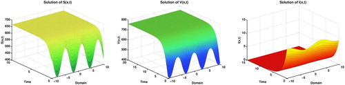
Example 4.2

Now let the system parameters are: $a = 1000, b = 5, q_{1} = 0.0001, q_{2} = 0.000001, m = 0.1, n = 0.1, c = 0.01.$ Then the formula (Equation10(10) $R_{0} = \frac{a b q_{1}}{(m + n) (m + c)} + \frac{a b n q_{2}}{m (m + n) (m + c)}$ (10) ) gives us the basic reproduction number as $R_{0} = 22.9545 > 1$ which ensures by Theorem 3.4 that, these values of parameters leads us to the disease equilibrium results as shown in Figure .

Figure 3. Disease equilibrium of the model (Equation2(2) $\begin{aligned} \begin{aligned} \frac{\partial S}{\partial t} & = δ_{1} Δ S + a - b q_{1} \frac{I (x, t)}{1 + I (x, t)} S (x, t) - (m + n) S (x, t) + c I (x, t) & i n A, \\ \frac{\partial V}{\partial t} & = δ_{2} Δ V + n S (x, t) - b q_{2} \frac{I (x, t)}{1 + I (x, t)} V (x, t) - m V (x, t) & i n A, \\ \frac{\partial I}{\partial t} & = δ_{3} Δ I + b (q_{1} S (x, t) + q_{2} V (x, t)) \frac{I (x, t)}{1 + I (x, t)} - m I (x, t) - c I (x, t) & i n A . \end{aligned} \end{aligned}$ (2) ) with time and spatial domain.

Figure 3. Disease equilibrium of the model (Equation2(2) ∂S∂t=δ1ΔS+a−bq1I(x,t)1+I(x,t)S(x,t)−m+nS(x,t)+cI(x,t)in A,∂V∂t=δ2ΔV+nS(x,t)−bq2I(x,t)1+I(x,t)V(x,t)−mV(x,t)in A,∂I∂t=δ3ΔI+bq1S(x,t)+q2V(x,t)I(x,t)1+I(x,t)−mI(x,t)−cI(x,t)in A.(2) ) with time and spatial domain.

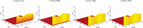
4.1. Parameter bifurcation observations

Now we are interested to know how the system (Equation2(2) $\begin{aligned} \begin{aligned} \frac{\partial S}{\partial t} & = δ_{1} Δ S + a - b q_{1} \frac{I (x, t)}{1 + I (x, t)} S (x, t) - (m + n) S (x, t) + c I (x, t) & i n A, \\ \frac{\partial V}{\partial t} & = δ_{2} Δ V + n S (x, t) - b q_{2} \frac{I (x, t)}{1 + I (x, t)} V (x, t) - m V (x, t) & i n A, \\ \frac{\partial I}{\partial t} & = δ_{3} Δ I + b (q_{1} S (x, t) + q_{2} V (x, t)) \frac{I (x, t)}{1 + I (x, t)} - m I (x, t) - c I (x, t) & i n A . \end{aligned} \end{aligned}$ (2) ) responses for different values of the system parameters.

From these Figures (Figure ), we clearly see that the disease is being extincted faster as c is increasing. But when c is more than $24.0$ then c has no valuable effect for the disease for this parametric setup and more interestingly we get a cusp at $t = 0$ .

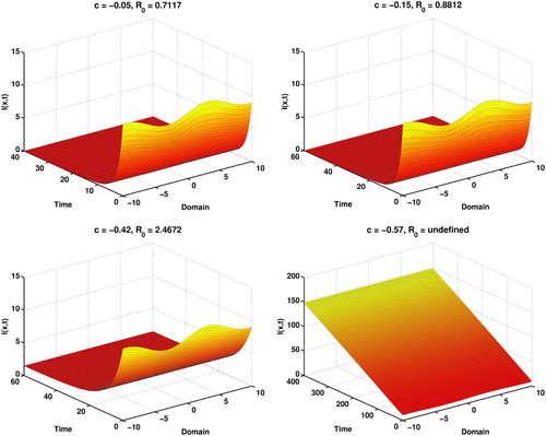
Figure 4. Bifurcation over therapeutic treatment impact c for $a = 1000, b = 5, q_{1} = 0.0001, q_{2} = 0.000001, m = 0.57, n = 0.1$ .

Though, in our system (Equation2(2) $\begin{aligned} \begin{aligned} \frac{\partial S}{\partial t} & = δ_{1} Δ S + a - b q_{1} \frac{I (x, t)}{1 + I (x, t)} S (x, t) - (m + n) S (x, t) + c I (x, t) & i n A, \\ \frac{\partial V}{\partial t} & = δ_{2} Δ V + n S (x, t) - b q_{2} \frac{I (x, t)}{1 + I (x, t)} V (x, t) - m V (x, t) & i n A, \\ \frac{\partial I}{\partial t} & = δ_{3} Δ I + b (q_{1} S (x, t) + q_{2} V (x, t)) \frac{I (x, t)}{1 + I (x, t)} - m I (x, t) - c I (x, t) & i n A . \end{aligned} \end{aligned}$ (2) ) we assumed c to be non-negative anyhow; but if the disease causing environment still predominates, then we may consider c to be negative, for example, $c \in [- m, 0)$ . And in that scenario, we get the following results,

Figure shows that, if c is negative i.e. in disease causing environment when basic reproduction number $R_{0} < 0.001$ , then it is a disease-free equilibrium while $R_{0} > 0.001$ reveals disease equilibrium. We also see the infection is increasing in a constant rate very roughly when $R_{0}$ is undefined in the case of $c = - m$ .

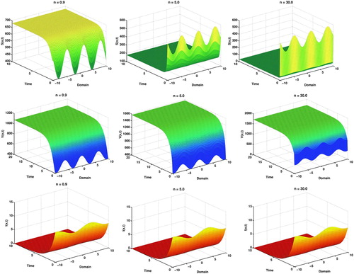
Figure 5. Bifurcation over therapeutic treatment impact c for $a = 1000, b = 5, q_{1} = 0.0001, q_{2} = 0.000001, m = 0.57, n = 0.8$ .

Here, in Figure , we clearly observe the impacts of vaccination coverage parameter n over susceptible $(S)$ and vaccinated $(V)$ individuals. Susceptible $(S)$ count converges to a minimum level and vaccinated $(V)$ count increases to a maximum level as n growing large. But infectious $(I)$ count remains approximately same for each cases.

Figure 6. Bifurcation over vaccination coverage impact n for $a = 1000, b = 5, q_{1} = 0.0001, q_{2} = 0.000001, m = 0.57, c = 0.25$ .

5. Auxiliary results and proofs

5.1. Existence and uniqueness of solution

In this portion, we prove the existence and uniqueness of the solution of the system (Equation2(2) $\begin{aligned} \begin{aligned} \frac{\partial S}{\partial t} & = δ_{1} Δ S + a - b q_{1} \frac{I (x, t)}{1 + I (x, t)} S (x, t) - (m + n) S (x, t) + c I (x, t) & i n A, \\ \frac{\partial V}{\partial t} & = δ_{2} Δ V + n S (x, t) - b q_{2} \frac{I (x, t)}{1 + I (x, t)} V (x, t) - m V (x, t) & i n A, \\ \frac{\partial I}{\partial t} & = δ_{3} Δ I + b (q_{1} S (x, t) + q_{2} V (x, t)) \frac{I (x, t)}{1 + I (x, t)} - m I (x, t) - c I (x, t) & i n A . \end{aligned} \end{aligned}$ (2) ) by learning the algorithm partially from a similar study of Xu et al. [Citation36].

Let us denote the subset of $R^{3}$ with vectors $x \geq 0$ as $R_{+}^{3}$ and $X := C (Ω, R)$ be a Banach space with the supremum norm $∥ \cdot ∥_{X}$ . Also we define $X^{+} := C (Ω, R_{+}^{3})$ then $(X, X^{+})$ is a strongly ordered space. Suppose that $(T_{1} (t), T_{2} (t), T_{3} (t)) : C (Ω, R) \to C (Ω, R)$ is the $C_{0}$ semigroups associated with $δ_{1} Δ - (m + n), δ_{2} Δ - m$ and $δ_{3} Δ - (m + c)$ subject to the Neumann boundary conditions, respectively. Then it follows that for any $ρ \in C (Ω, R)$ and $t \geq 0$ $\begin{aligned} (T_{1} (t) ρ) (x) & = e^{- (m + n) t} \int_{Ω} Γ_{1} (x, y, t) ρ (y) d x \\ (T_{2} (t) ρ) (x) & = e^{- m t} \int_{Ω} Γ_{2} (x, y, t) ρ (y) d x \\ (T_{3} (t) ρ) (x) & = e^{- (m + c) t} \int_{Ω} Γ_{3} (x, y, t) ρ (y) d x \end{aligned}$ where, $Γ_{i}, i = 1, 2, 3$ are the Green functions associated with $δ_{i} Δ, i = 1, 2, 3$ , subject to the Neumann boundary conditions, respectively. It then follows from [Citation29] that the function $T_{i} (t) : C (Ω, R) \to C (Ω, R), i = 1, 2, 3, f o r a l l t > 0$ is compact and strongly positive. Particularly, $T (t) = (T_{1} (t), T_{2} (t), T_{3} (t)) : C (Ω, R) \to C (Ω, R), \forall t \geq 0$ is a strongly continuous semigroup.

If $A_{i} : G (A_{i}) \to X$ is the generator of $T_{i}, i = 1, 2, 3$ , then $T (t) = (T_{1} (t), T_{2} (t), T_{3} (t)) : X \to X$ is a semigroup generated by the operator $A = (A_{1}, A_{2}, A_{3})$ which is defined on $G (A) := G (A_{1}) \times G (A_{2}) \times G (A_{3})$ . Now for any $ρ = (ρ_{1}, ρ_{2}, ρ_{3}) \in X$ , let us define $F = (F_{1}, F_{2}, F_{3}) : X^{+} \to X$ by: $\begin{aligned} \begin{array}{lll} F_{1} (ρ) (x) = a - b q_{1} \frac{ρ_{3} (x)}{1 + ρ_{3} (x)} ρ_{1} (x) - (m + n) ρ_{1} (x) + c ρ_{3} (x), & \forall x \in Ω \\ F_{2} (ρ) (x) = n ρ_{1} (x) - b q_{2} \frac{ρ_{3} (x)}{1 + ρ_{3} (x)} ρ_{2} (x) - m ρ_{2} (x), & \forall x \in Ω \\ F_{3} (ρ) (x) = b q_{1} \frac{ρ_{3} (x)}{1 + ρ_{3} (x)} ρ_{1} (x) + b q_{2} \frac{ρ_{3} (x)}{1 + ρ_{3} (x)} ρ_{2} (x) - (m + c) ρ_{3} (x), & \forall x \in Ω . \end{array} \end{aligned}$ Using these operators, we can write (Equation2(2) $\begin{aligned} \begin{aligned} \frac{\partial S}{\partial t} & = δ_{1} Δ S + a - b q_{1} \frac{I (x, t)}{1 + I (x, t)} S (x, t) - (m + n) S (x, t) + c I (x, t) & i n A, \\ \frac{\partial V}{\partial t} & = δ_{2} Δ V + n S (x, t) - b q_{2} \frac{I (x, t)}{1 + I (x, t)} V (x, t) - m V (x, t) & i n A, \\ \frac{\partial I}{\partial t} & = δ_{3} Δ I + b (q_{1} S (x, t) + q_{2} V (x, t)) \frac{I (x, t)}{1 + I (x, t)} - m I (x, t) - c I (x, t) & i n A . \end{aligned} \end{aligned}$ (2) )–(Equation4(4) $\frac{\partial S}{\partial ω} (x, t) = \frac{\partial V}{\partial ω} (x, t) = \frac{\partial I}{\partial ω} (x, t) = 0 o n \partial A .$ (4) ) as the following integral equation $u (t) = T (t) ρ + \int_{0}^{t} T (t - s) F (u (s)) d s,$ where, $u (t) = (\begin{matrix} S (t) \\ V (t) \\ I (t) \end{matrix}), T (t) = (\begin{matrix} T_{1} (t) & 0 & 0 \\ 0 & T_{2} (t) & 0 \\ 0 & 0 & T_{3} (t) \end{matrix}) .$ It can also be rewritten as the following abstract differential equation (11) $\begin{aligned} \frac{d u}{d t} = A u + F (u), t > 0, \\ u_{0} = ρ \in X^{+}, \end{aligned}$ (11) where, $u = (S, V, I)$ and $ρ = (S_{0}, V_{0}, I_{0})$ .

Since $F (ρ)$ is local Lipschitz continuous on $X^{+}$ , it then follows that for any $ρ \in X^{+}$ , (Equation11(11) $\begin{aligned} \frac{d u}{d t} = A u + F (u), t > 0, \\ u_{0} = ρ \in X^{+}, \end{aligned}$ (11) ) admits a unique noncontinuous mild solution $u (\cdot, t, ρ)$ such that $u (\cdot, t, ρ) \in X$ for all t in its maximum interval of existence. Moreover, it follows from ([Citation35], Corollary 2.2.5) that $u (\cdot, t, ρ)$ is a class solution of (Equation2(2) $\begin{aligned} \begin{aligned} \frac{\partial S}{\partial t} & = δ_{1} Δ S + a - b q_{1} \frac{I (x, t)}{1 + I (x, t)} S (x, t) - (m + n) S (x, t) + c I (x, t) & i n A, \\ \frac{\partial V}{\partial t} & = δ_{2} Δ V + n S (x, t) - b q_{2} \frac{I (x, t)}{1 + I (x, t)} V (x, t) - m V (x, t) & i n A, \\ \frac{\partial I}{\partial t} & = δ_{3} Δ I + b (q_{1} S (x, t) + q_{2} V (x, t)) \frac{I (x, t)}{1 + I (x, t)} - m I (x, t) - c I (x, t) & i n A . \end{aligned} \end{aligned}$ (2) ) with Neumann boundary conditions (Equation4(4) $\frac{\partial S}{\partial ω} (x, t) = \frac{\partial V}{\partial ω} (x, t) = \frac{\partial I}{\partial ω} (x, t) = 0 o n \partial A .$ (4) ) for all $t > 0$ . Further, by the scalar parabolic maximum principle, we see from the equation in (Equation2(2) $\begin{aligned} \begin{aligned} \frac{\partial S}{\partial t} & = δ_{1} Δ S + a - b q_{1} \frac{I (x, t)}{1 + I (x, t)} S (x, t) - (m + n) S (x, t) + c I (x, t) & i n A, \\ \frac{\partial V}{\partial t} & = δ_{2} Δ V + n S (x, t) - b q_{2} \frac{I (x, t)}{1 + I (x, t)} V (x, t) - m V (x, t) & i n A, \\ \frac{\partial I}{\partial t} & = δ_{3} Δ I + b (q_{1} S (x, t) + q_{2} V (x, t)) \frac{I (x, t)}{1 + I (x, t)} - m I (x, t) - c I (x, t) & i n A . \end{aligned} \end{aligned}$ (2) ) that $S (x, t), V (x, t)$ and $I (x, t)$ are all non-negative. Therefore, we obtain the following basic result on solution of the governing system (Equation2(2) $\begin{aligned} \begin{aligned} \frac{\partial S}{\partial t} & = δ_{1} Δ S + a - b q_{1} \frac{I (x, t)}{1 + I (x, t)} S (x, t) - (m + n) S (x, t) + c I (x, t) & i n A, \\ \frac{\partial V}{\partial t} & = δ_{2} Δ V + n S (x, t) - b q_{2} \frac{I (x, t)}{1 + I (x, t)} V (x, t) - m V (x, t) & i n A, \\ \frac{\partial I}{\partial t} & = δ_{3} Δ I + b (q_{1} S (x, t) + q_{2} V (x, t)) \frac{I (x, t)}{1 + I (x, t)} - m I (x, t) - c I (x, t) & i n A . \end{aligned} \end{aligned}$ (2) )–(Equation4(4) $\frac{\partial S}{\partial ω} (x, t) = \frac{\partial V}{\partial ω} (x, t) = \frac{\partial I}{\partial ω} (x, t) = 0 o n \partial A .$ (4) ).

Lemma 5.1

For any initial value function $ρ = (ρ_{1}, ρ_{2}, ρ_{3}) \in X^{+}$ , system (Equation2(2) $\begin{aligned} \begin{aligned} \frac{\partial S}{\partial t} & = δ_{1} Δ S + a - b q_{1} \frac{I (x, t)}{1 + I (x, t)} S (x, t) - (m + n) S (x, t) + c I (x, t) & i n A, \\ \frac{\partial V}{\partial t} & = δ_{2} Δ V + n S (x, t) - b q_{2} \frac{I (x, t)}{1 + I (x, t)} V (x, t) - m V (x, t) & i n A, \\ \frac{\partial I}{\partial t} & = δ_{3} Δ I + b (q_{1} S (x, t) + q_{2} V (x, t)) \frac{I (x, t)}{1 + I (x, t)} - m I (x, t) - c I (x, t) & i n A . \end{aligned} \end{aligned}$ (2) )–(Equation4(4) $\frac{\partial S}{\partial ω} (x, t) = \frac{\partial V}{\partial ω} (x, t) = \frac{\partial I}{\partial ω} (x, t) = 0 o n \partial A .$ (4) ) has a unique solution $u (x, t, ρ)$ on $[0, σ_{ρ})$ with $u (x, t, ρ) = ρ$ and $u (\cdot, t, ρ) \in X^{+}, \forall t \in [0, σ_{ρ})$ , where $σ_{ρ} \leq \infty$ .

Next, we show that the solution of the system (Equation2(2) $\begin{aligned} \begin{aligned} \frac{\partial S}{\partial t} & = δ_{1} Δ S + a - b q_{1} \frac{I (x, t)}{1 + I (x, t)} S (x, t) - (m + n) S (x, t) + c I (x, t) & i n A, \\ \frac{\partial V}{\partial t} & = δ_{2} Δ V + n S (x, t) - b q_{2} \frac{I (x, t)}{1 + I (x, t)} V (x, t) - m V (x, t) & i n A, \\ \frac{\partial I}{\partial t} & = δ_{3} Δ I + b (q_{1} S (x, t) + q_{2} V (x, t)) \frac{I (x, t)}{1 + I (x, t)} - m I (x, t) - c I (x, t) & i n A . \end{aligned} \end{aligned}$ (2) )–(Equation4(4) $\frac{\partial S}{\partial ω} (x, t) = \frac{\partial V}{\partial ω} (x, t) = \frac{\partial I}{\partial ω} (x, t) = 0 o n \partial A .$ (4) ) with the initial value function $ρ \in X^{+}$ actually exists globally, that is, $σ = \infty$ . To this end, we need the following result ([Citation21], Lemma 5.1).

Consider the following reaction-diffusion equation (12) $\begin{aligned} \begin{array}{lll} \frac{\partial v (x, t)}{\partial t} = D Δ v (x, t) + A - d v (x, t), & i n A, \\ \frac{\partial v}{\partial ω} (x, t) = 0, & o n \partial A, \end{array} \end{aligned}$ (12) where $D > 0, A > 0$ and $d > 0$ are positive constants.

Lemma 5.2

The system (Equation12(12) $\begin{aligned} \begin{array}{lll} \frac{\partial v (x, t)}{\partial t} = D Δ v (x, t) + A - d v (x, t), & i n A, \\ \frac{\partial v}{\partial ω} (x, t) = 0, & o n \partial A, \end{array} \end{aligned}$ (12) ) admits a unique positive steady state $v^{*} = \frac{A}{d}$ which is globally attractive in $C (Ω, R)$ .

Now we are ready to produce the proof of the Theorem 3.1.

Proof of Theorem 3.1.

By Lemma 5.1, the system (Equation2(2) $\begin{aligned} \begin{aligned} \frac{\partial S}{\partial t} & = δ_{1} Δ S + a - b q_{1} \frac{I (x, t)}{1 + I (x, t)} S (x, t) - (m + n) S (x, t) + c I (x, t) & i n A, \\ \frac{\partial V}{\partial t} & = δ_{2} Δ V + n S (x, t) - b q_{2} \frac{I (x, t)}{1 + I (x, t)} V (x, t) - m V (x, t) & i n A, \\ \frac{\partial I}{\partial t} & = δ_{3} Δ I + b (q_{1} S (x, t) + q_{2} V (x, t)) \frac{I (x, t)}{1 + I (x, t)} - m I (x, t) - c I (x, t) & i n A . \end{aligned} \end{aligned}$ (2) )–(Equation4(4) $\frac{\partial S}{\partial ω} (x, t) = \frac{\partial V}{\partial ω} (x, t) = \frac{\partial I}{\partial ω} (x, t) = 0 o n \partial A .$ (4) ) has a unique solution $u (\cdot, t, ρ)$ on $[0, σ_{ρ})$ and $u (x, t, ρ) \geq 0$ for any $t \in [0, σ_{ρ})$ and $x \in Ω$ .

Now, let define the total population (13) $N (x, t) = S (x, t) + V (x, t) + I (x, t)$ (13) and recall the primary assumption of Theorem 3.1 statement: $δ_{1} = δ_{2} = δ_{3} =: Λ$ . Then (14) $\begin{aligned} \frac{\partial N (x, t)}{\partial t} & = \frac{\partial S (x, t)}{\partial t} + \frac{\partial V (x, t)}{\partial t} + \frac{\partial I (x, t)}{\partial t} \\ = Λ Δ S + a - b q_{1} \frac{I (x, t)}{1 + I (x, t)} S (x, t) - (m + n) S (x, t) + c I (x, t) \\ + Λ Δ V + n S (x, t) - b q_{2} \frac{I (x, t)}{1 + I (x, t)} V (x, t) - m V (x, t) \\ + Λ Δ I + b (q_{1} S (x, t) + q_{2} V (x, t)) \frac{I (x, t)}{1 + I (x, t)} - m I (x, t) - c I (x, t) \\ = Λ N (x, t) + a - m N (x, t) . \end{aligned}$ (14) It follows from Lemma 5.2 that $\frac{a}{m}$ is a global attractor for the reaction-diffusion Equation (Equation14(14) $\begin{aligned} \frac{\partial N (x, t)}{\partial t} & = \frac{\partial S (x, t)}{\partial t} + \frac{\partial V (x, t)}{\partial t} + \frac{\partial I (x, t)}{\partial t} \\ = Λ Δ S + a - b q_{1} \frac{I (x, t)}{1 + I (x, t)} S (x, t) - (m + n) S (x, t) + c I (x, t) \\ + Λ Δ V + n S (x, t) - b q_{2} \frac{I (x, t)}{1 + I (x, t)} V (x, t) - m V (x, t) \\ + Λ Δ I + b (q_{1} S (x, t) + q_{2} V (x, t)) \frac{I (x, t)}{1 + I (x, t)} - m I (x, t) - c I (x, t) \\ = Λ N (x, t) + a - m N (x, t) . \end{aligned}$ (14) ).

By (Equation14(14) $\begin{aligned} \frac{\partial N (x, t)}{\partial t} & = \frac{\partial S (x, t)}{\partial t} + \frac{\partial V (x, t)}{\partial t} + \frac{\partial I (x, t)}{\partial t} \\ = Λ Δ S + a - b q_{1} \frac{I (x, t)}{1 + I (x, t)} S (x, t) - (m + n) S (x, t) + c I (x, t) \\ + Λ Δ V + n S (x, t) - b q_{2} \frac{I (x, t)}{1 + I (x, t)} V (x, t) - m V (x, t) \\ + Λ Δ I + b (q_{1} S (x, t) + q_{2} V (x, t)) \frac{I (x, t)}{1 + I (x, t)} - m I (x, t) - c I (x, t) \\ = Λ N (x, t) + a - m N (x, t) . \end{aligned}$ (14) ), for any $ρ \in X^{+}$ , we see that there exist some $t_{1} = t_{1} (ρ) > 0$ such that $N (x, t) \leq \frac{a}{m} + 1 := M, \forall t \geq t_{1}, x \in Ω .$ Now, according to (Equation13(13) $N (x, t) = S (x, t) + V (x, t) + I (x, t)$ (13) ), as the first equation of (Equation2(2) $\begin{aligned} \begin{aligned} \frac{\partial S}{\partial t} & = δ_{1} Δ S + a - b q_{1} \frac{I (x, t)}{1 + I (x, t)} S (x, t) - (m + n) S (x, t) + c I (x, t) & i n A, \\ \frac{\partial V}{\partial t} & = δ_{2} Δ V + n S (x, t) - b q_{2} \frac{I (x, t)}{1 + I (x, t)} V (x, t) - m V (x, t) & i n A, \\ \frac{\partial I}{\partial t} & = δ_{3} Δ I + b (q_{1} S (x, t) + q_{2} V (x, t)) \frac{I (x, t)}{1 + I (x, t)} - m I (x, t) - c I (x, t) & i n A . \end{aligned} \end{aligned}$ (2) ) is local Lipschitz continuous on $X^{+}$ , it can easily be said that, for any $ρ \in X^{+}$ , there exist some $t_{1} = t_{1} (ρ) > 0$ such that $S (x, t) \leq M_{1}, \forall t \geq t_{1}, x \in Ω .$ Then by the similar argument as above, we also show that there are $M_{i} > 0$ , independent of the choice of $ρ \in X^{+}$ , and $t_{i} = t_{i} (ρ) > 0, i = 1, 2, 3$ , such that $V (x, t) \leq M_{2}, I (x, t) \leq M_{3}, \forall t \geq t_{1}, x \in Ω .$ Therefore, the non-negative solution of (Equation2(2) $\begin{aligned} \begin{aligned} \frac{\partial S}{\partial t} & = δ_{1} Δ S + a - b q_{1} \frac{I (x, t)}{1 + I (x, t)} S (x, t) - (m + n) S (x, t) + c I (x, t) & i n A, \\ \frac{\partial V}{\partial t} & = δ_{2} Δ V + n S (x, t) - b q_{2} \frac{I (x, t)}{1 + I (x, t)} V (x, t) - m V (x, t) & i n A, \\ \frac{\partial I}{\partial t} & = δ_{3} Δ I + b (q_{1} S (x, t) + q_{2} V (x, t)) \frac{I (x, t)}{1 + I (x, t)} - m I (x, t) - c I (x, t) & i n A . \end{aligned} \end{aligned}$ (2) )–(Equation4(4) $\frac{\partial S}{\partial ω} (x, t) = \frac{\partial V}{\partial ω} (x, t) = \frac{\partial I}{\partial ω} (x, t) = 0 o n \partial A .$ (4) ) is ultimately bounded with respect to the maximum norm. This means that the solution semiflow $Φ (t) : X^{+} \to X^{+}$ defined by $(Φ (t) ρ) (x) = u (x, t, ρ), x \in Ω$ , is point dissipative. In view of [Citation35], $Φ (t)$ is compact for any $t > 0$ . Thus, [Citation11] implies that $Φ (t) : X^{+} \to X^{+}, t \geq 0$ , has a global compact attractor in $X^{+}$ .

This completes the proof.

5.2. Analysis of local steady states

In this section, we want to explain the local stability of the equilibria for the system (Equation2(2) $\begin{aligned} \begin{aligned} \frac{\partial S}{\partial t} & = δ_{1} Δ S + a - b q_{1} \frac{I (x, t)}{1 + I (x, t)} S (x, t) - (m + n) S (x, t) + c I (x, t) & i n A, \\ \frac{\partial V}{\partial t} & = δ_{2} Δ V + n S (x, t) - b q_{2} \frac{I (x, t)}{1 + I (x, t)} V (x, t) - m V (x, t) & i n A, \\ \frac{\partial I}{\partial t} & = δ_{3} Δ I + b (q_{1} S (x, t) + q_{2} V (x, t)) \frac{I (x, t)}{1 + I (x, t)} - m I (x, t) - c I (x, t) & i n A . \end{aligned} \end{aligned}$ (2) ). Thus we consider the proof of our second result, Theorem 3.2.

Proof of Theorem 3.2.

By linearizing the system (Equation2(2) $\begin{aligned} \begin{aligned} \frac{\partial S}{\partial t} & = δ_{1} Δ S + a - b q_{1} \frac{I (x, t)}{1 + I (x, t)} S (x, t) - (m + n) S (x, t) + c I (x, t) & i n A, \\ \frac{\partial V}{\partial t} & = δ_{2} Δ V + n S (x, t) - b q_{2} \frac{I (x, t)}{1 + I (x, t)} V (x, t) - m V (x, t) & i n A, \\ \frac{\partial I}{\partial t} & = δ_{3} Δ I + b (q_{1} S (x, t) + q_{2} V (x, t)) \frac{I (x, t)}{1 + I (x, t)} - m I (x, t) - c I (x, t) & i n A . \end{aligned} \end{aligned}$ (2) ) at $E_{0}$ , we get $\frac{\partial u}{\partial t} = δ Δ u (x, t) + κ_{1} u (x, t),$ where, $\begin{aligned} δ & = (\begin{matrix} δ_{1} & 0 & 0 \\ 0 & δ_{2} & 0 \\ 0 & 0 & δ_{3} \end{matrix}), \\ κ_{1} & = (\begin{matrix} - (m + n) & 0 & - b q_{1} S_{0} + c \\ n & - m & - b q_{2} V_{0} \\ 0 & 0 & b q_{1} S_{0} + b q_{2} V_{0} - (m + c) \end{matrix}) . \end{aligned}$ Then, we can obtain the following characteristic polynomial $| λ I + δ L^{2} - κ_{1} | = 0,$ where, λ is the eigenvalue which determines temporal growth, $I$ is the $3 \times 3$ identity matrix and $L$ is the wave-number [Citation24]. Then, we have (15) $(λ + δ_{1} L^{2} + m + n) (λ + δ_{2} L^{2} + m) (λ + δ_{3} L^{2} + m + c - b q_{1} S_{0} - b q_{2} V_{0}) = 0.$ (15) Now, it is clear that $\begin{aligned} λ_{1} & = - (δ_{1} L^{2} + m + n) < 0, \\ λ_{2} & = - (δ_{1} L^{3} + m) < 0, \\ a n d λ_{3} & = - (δ_{3} L^{2} + m + c - b q_{1} S_{0} - b q_{2} V_{0}) \\ = - (δ_{3} L^{2} + (m + c) (1 - R_{0})) . \end{aligned}$ It follows from $R_{0} < 1$ that $E_{0}$ is locally asymptotically stable.

In the following, we prove the second part of the theorem. Linearizing the system (Equation2(2) $\begin{aligned} \begin{aligned} \frac{\partial S}{\partial t} & = δ_{1} Δ S + a - b q_{1} \frac{I (x, t)}{1 + I (x, t)} S (x, t) - (m + n) S (x, t) + c I (x, t) & i n A, \\ \frac{\partial V}{\partial t} & = δ_{2} Δ V + n S (x, t) - b q_{2} \frac{I (x, t)}{1 + I (x, t)} V (x, t) - m V (x, t) & i n A, \\ \frac{\partial I}{\partial t} & = δ_{3} Δ I + b (q_{1} S (x, t) + q_{2} V (x, t)) \frac{I (x, t)}{1 + I (x, t)} - m I (x, t) - c I (x, t) & i n A . \end{aligned} \end{aligned}$ (2) ) at $E^{*}$ , we obtain $\frac{\partial u}{\partial t} = δ Δ u (x, t) + κ_{2} u (x, t),$ where, $\begin{aligned} κ_{2} & = (\begin{matrix} - (m + n + b q_{1} \frac{I^{*}}{1 + I^{*}}) & 0 \\ n & - (m + b q_{2} \frac{I^{*}}{1 + I^{*}}) \\ b q_{1} \frac{I^{*}}{1 + I^{*}} & b q_{2} \frac{I^{*}}{1 + I^{*}} \end{matrix} \\ \begin{matrix} c - b q_{1} \frac{1}{(1 + I^{*})^{2}} S^{*} \\ - b q_{2} \frac{1}{(1 + I^{*})^{2}} V^{*} \\ b (q_{1} S^{*} + q_{2} V^{*}) \frac{1}{(1 + I^{*})^{2}} - (m + c) \end{matrix}) . \end{aligned}$ Then we obtain the following characteristic equation (16) $λ^{3} + G_{1} (L^{2}) λ^{2} + G_{2} (L^{2}) λ + G_{3} (L^{2}) = 0$ (16) where, $\begin{aligned} G_{1} (L^{2}) & = δ_{1} L^{2} + m + n + b q_{1} \frac{I^{*}}{1 + I^{*}} + δ_{2} L^{2} + m + b q_{2} \frac{I^{*}}{1 + I^{*}} \\ + δ_{3} L^{2} + m + c - b (q_{1} S^{*} + q_{2} V^{*}) \frac{I^{*}}{1 + I^{*}}, \\ G_{2} (L^{2}) & = (δ_{2} L^{2} + m + b q_{2} \frac{I^{*}}{1 + I^{*}}) (δ_{3} L^{2} + m + c) + b q_{1} S^{*} \frac{1}{(1 + I^{*})^{2}} b q_{1} \frac{I^{*}}{1 + I^{*}} \\ + (δ_{1} L^{2} + m + n + b q_{1} \frac{I^{*}}{1 + I^{*}}) \\ \times (δ_{2} L^{2} + m + b q_{2} \frac{I^{*}}{1 + I^{*}} + δ_{3} L^{2} + m + c) \\ + b q_{2} V^{*} \frac{1}{(1 + I^{*})^{2}} b q_{2} \frac{I^{*}}{1 + I^{*}} \\ - (δ_{1} L^{2} + m + n + b q_{1} \frac{I^{*}}{1 + I^{*}} + δ_{2} L^{2} + m + b q_{2} \frac{I^{*}}{1 + I^{*}}) \\ \times (b q_{1} S^{*} \frac{1}{(1 + I^{*})^{2}} + b q_{2} V^{*} \frac{1}{(1 + I^{*})^{2}}), \\ G_{3} (L^{2}) = & (δ_{1} L^{2} + m + n + b q_{1} \frac{I^{*}}{1 + I^{*}}) (δ_{2} L^{2} + m + b q_{2} \frac{I^{*}}{1 + I^{*}}) (δ_{3} L^{2} + m + c) \\ + b q_{2} V^{*} \frac{1}{(1 + I^{*})^{2}} b q_{2} \frac{I^{*}}{1 + I^{*}} (δ_{3} L^{2} + m + c) + n b q_{1} S^{*} \frac{1}{(1 + I^{*})^{2}} b q_{2} \frac{I^{*}}{1 + I^{*}} \\ + b q_{1} S^{*} \frac{1}{(1 + I^{*})^{2}} b q_{1} \frac{I^{*}}{1 + I^{*}} (δ_{2} L^{2} + m + b q_{2} \frac{I^{*}}{1 + I^{*}}) \\ - (δ_{1} L^{2} + m + n + b q_{1} \frac{I^{*}}{1 + I^{*}}) (δ_{2} L^{2} + m + b q_{2} \frac{I^{*}}{1 + I^{*}}) \\ \times (b q_{1} S^{*} \frac{1}{(1 + I^{*})^{2}} + b q_{2} V^{*} \frac{1}{(1 + I^{*})^{2}}) \\ - b q_{2} \frac{I^{*}}{1 + I^{*}} b q_{2} \frac{1}{(1 + I^{*})^{2}} (b q_{1} S^{*} \frac{1}{(1 + I^{*})^{2}} + b q_{2} V^{*} \frac{1}{(1 + I^{*})^{2}}) . \end{aligned}$ Now, let us take $b q_{1} S^{*} \frac{1}{(1 + I^{*})^{2}} + b q_{2} V^{*} \frac{1}{(1 + I^{*})^{2}} \leq b (q_{1} S^{*} + q_{2} V^{*}) \frac{1}{1 + I^{*}} = m + c,$ then we can get $\begin{aligned} G_{1} (L^{2}) & \geq δ_{1} L^{2} + m + n + b q_{1} \frac{I^{*}}{1 + I^{*}} + δ_{2} L^{2} + m + b q_{2} \frac{I^{*}}{1 + I^{*}} + δ_{3} L^{2} > 0, \\ G_{2} (L^{2}) & > δ_{3} L^{2} (δ_{2} L^{2} + m + b q_{2} \frac{I^{*}}{1 + I^{*}}) > 0, \\ G_{3} (L^{2}) & > (δ_{1} L^{2} + m + n + b q_{1} \frac{I^{*}}{1 + I^{*}}) (δ_{2} L^{2} + m + b q_{2} \frac{I^{*}}{1 + I^{*}}) δ_{3} L^{2} > 0. \end{aligned}$ These lead us to the following conclusion $G_{1} (L^{2}) G_{2} (L^{2}) - G_{3} (L^{2}) > b q_{2} \frac{I^{*}}{1 + I^{*}} b q_{2} V^{*} \frac{1}{(1 + I^{*})^{2}} b (q_{1} S^{*} + q_{2} V^{*}) \frac{1}{(1 + I^{*})^{2}} > 0.$ By the Routh-Hurwitz criterion, we know that all eigenvalues of (Equation16(16) $λ^{3} + G_{1} (L^{2}) λ^{2} + G_{2} (L^{2}) λ + G_{3} (L^{2}) = 0$ (16) ) have negative real parts. It means that the disease equilibrium $E^{*}$ of system (Equation16(16) $λ^{3} + G_{1} (L^{2}) λ^{2} + G_{2} (L^{2}) λ + G_{3} (L^{2}) = 0$ (16) ) is locally asymptotically stable when $R_{0} > 1$ .

5.3. Global stability analysis

In this section, we investigate the global stability of the two constant equilibria $E_{0} a n d E^{*}$ in the case of a bounded domain Ω in which $(S (x, t), V (x, t), I (x, t))$ is an arbitrary positive solution of the system (Equation2(2) $\begin{aligned} \begin{aligned} \frac{\partial S}{\partial t} & = δ_{1} Δ S + a - b q_{1} \frac{I (x, t)}{1 + I (x, t)} S (x, t) - (m + n) S (x, t) + c I (x, t) & i n A, \\ \frac{\partial V}{\partial t} & = δ_{2} Δ V + n S (x, t) - b q_{2} \frac{I (x, t)}{1 + I (x, t)} V (x, t) - m V (x, t) & i n A, \\ \frac{\partial I}{\partial t} & = δ_{3} Δ I + b (q_{1} S (x, t) + q_{2} V (x, t)) \frac{I (x, t)}{1 + I (x, t)} - m I (x, t) - c I (x, t) & i n A . \end{aligned} \end{aligned}$ (2) ). First, let us consider the following shortcuts for convenience $S = S (x, t), V = V (x, t), I = I (x, t) .$ In case of global analysis, we consider the Lyapunov functional and the results varies with basic reproduction number. We stated two important results in the earlier Section 2.

At this phase, we are in stable setting to establish the Theorem 3.3 as long as the basic reporduction number $R_{0} \leq 1$ .

Proof of Theorem 3.3.

Let define a Lyapunov function as $V_{1} (t) = \int_{Ω} W_{1} (x, t) d x,$ where, $W_{1} (x, t) = S_{0} (\frac{S}{S_{0}} - 1 - \ln \frac{S}{S_{0}}) + V_{0} (\frac{V}{V_{0}} - 1 - \ln \frac{V}{V_{0}}) + I .$ Calculating the time derivative of $W_{1} (x, t)$ along the solution of (Equation2(2) $\begin{aligned} \begin{aligned} \frac{\partial S}{\partial t} & = δ_{1} Δ S + a - b q_{1} \frac{I (x, t)}{1 + I (x, t)} S (x, t) - (m + n) S (x, t) + c I (x, t) & i n A, \\ \frac{\partial V}{\partial t} & = δ_{2} Δ V + n S (x, t) - b q_{2} \frac{I (x, t)}{1 + I (x, t)} V (x, t) - m V (x, t) & i n A, \\ \frac{\partial I}{\partial t} & = δ_{3} Δ I + b (q_{1} S (x, t) + q_{2} V (x, t)) \frac{I (x, t)}{1 + I (x, t)} - m I (x, t) - c I (x, t) & i n A . \end{aligned} \end{aligned}$ (2) ) gives $\frac{\partial W_{1}}{\partial t} = (1 - \frac{S_{0}}{S}) \frac{\partial S}{\partial t} + (1 - \frac{V_{0}}{V}) \frac{\partial V}{\partial t} + \frac{\partial I}{\partial t} .$ Then from (Equation2(2) $\begin{aligned} \begin{aligned} \frac{\partial S}{\partial t} & = δ_{1} Δ S + a - b q_{1} \frac{I (x, t)}{1 + I (x, t)} S (x, t) - (m + n) S (x, t) + c I (x, t) & i n A, \\ \frac{\partial V}{\partial t} & = δ_{2} Δ V + n S (x, t) - b q_{2} \frac{I (x, t)}{1 + I (x, t)} V (x, t) - m V (x, t) & i n A, \\ \frac{\partial I}{\partial t} & = δ_{3} Δ I + b (q_{1} S (x, t) + q_{2} V (x, t)) \frac{I (x, t)}{1 + I (x, t)} - m I (x, t) - c I (x, t) & i n A . \end{aligned} \end{aligned}$ (2) ), we can write $\begin{aligned} \frac{\partial W_{1}}{\partial t} & = (1 - \frac{S_{0}}{S}) (δ_{1} Δ S + a - b q_{1} \frac{I}{1 + I} S - (m + n) S + c I) \\ + (1 - \frac{V_{0}}{V}) (δ_{2} Δ V + n S - b q_{2} \frac{I}{1 + I} V - m V) \\ + (δ_{3} Δ I + b q_{1} \frac{I}{1 + I} S + b q_{2} \frac{I}{1 + I} V - m I - c I) . \end{aligned}$ But, as $a = (m + n) S_{0} a n d m V_{0} = n S_{0}$ , we can write $\begin{aligned} \frac{\partial W_{1}}{\partial t} & = (1 - \frac{S_{0}}{S}) δ_{1} Δ S + (1 - \frac{V_{0}}{V}) δ_{2} Δ V + δ_{3} Δ I + m S_{0} (2 - \frac{S}{S_{0}} - \frac{S_{0}}{S}) \\ + n S_{0} (3 - \frac{S_{0}}{S} - \frac{V}{V_{0}} - \frac{S}{S_{0}} \frac{V_{0}}{V}) - (m + c) (1 + I - R_{0}) \frac{I}{1 + I} + (1 - \frac{S_{0}}{S}) c I . \end{aligned}$ By Green's formula and Neumann boundary conditions (Equation4(4) $\frac{\partial S}{\partial ω} (x, t) = \frac{\partial V}{\partial ω} (x, t) = \frac{\partial I}{\partial ω} (x, t) = 0 o n \partial A .$ (4) ), we get (17) $\int_{Ω} Δ S d x = \int_{\partial Ω} \frac{\partial S}{\partial ω} d S = 0.$ (17) Similarly, (18) $\int_{Ω} Δ V d x = \int_{Ω} Δ I d x = 0.$ (18) Again, by Green's formula and the Neumann boundary conditions (Equation4(4) $\frac{\partial S}{\partial ω} (x, t) = \frac{\partial V}{\partial ω} (x, t) = \frac{\partial I}{\partial ω} (x, t) = 0 o n \partial A .$ (4) ), we have the Green's first identity as $\int_{Ω} (\frac{Δ S}{S} - \frac{{∥ \nabla S ∥}^{2}}{S^{2}}) d x = \int_{\partial Ω} \frac{1}{S} (\nabla S \cdot ω) d S = 0,$ which implies (19) $\int_{Ω} \frac{Δ S}{S} d x = \int_{Ω} \frac{{∥ \nabla S ∥}^{2}}{S^{2}} d x .$ (19) By the same arguments, we also can write (20) $\begin{aligned} \int_{Ω} \frac{Δ V}{V} d x = \int_{Ω} \frac{{∥ \nabla V ∥}^{2}}{V^{2}} d x, \end{aligned}$ (20) (21) $\begin{aligned} a n d & \int_{Ω} \frac{Δ I}{I} d x = \int_{Ω} \frac{{∥ \nabla I ∥}^{2}}{I^{2}} d x . \end{aligned}$ (21) Then using the above arguments, we have (22) $\begin{aligned} \frac{d V_{1}}{d t} & = - δ_{1} S_{0} \int_{Ω} \frac{{∥ \nabla S ∥}^{2}}{S^{2}} d x - δ_{2} V_{0} \int_{Ω} \frac{{∥ \nabla V ∥}^{2}}{V^{2}} d x + m S_{0} \int_{Ω} (2 - \frac{S}{S_{0}} - \frac{S_{0}}{S}) d x \\ + n S_{0} \int_{Ω} (3 - \frac{S_{0}}{S} - \frac{V}{V_{0}} - \frac{S}{S_{0}} \frac{V_{0}}{V}) d x - (m + c) \int_{Ω} ((1 + I - R_{0}) \frac{I}{1 + I}) d x \\ + c \int_{Ω} I (1 - \frac{S_{0}}{S}) d x, \\ = - δ_{1} S_{0} \int_{Ω} \frac{{∥ \nabla S ∥}^{2}}{S^{2}} d x - δ_{2} V_{0} \int_{Ω} \frac{{∥ \nabla V ∥}^{2}}{V^{2}} d x - m S_{0} \int_{Ω} \frac{(S - S_{0})^{2}}{S_{0} S} d x \\ - n S_{0} \int_{Ω} (\frac{S_{0}}{S} + \frac{V}{V_{0}} + \frac{S}{S_{0}} \frac{V_{0}}{V} - 3) d x - (m + c) \int_{Ω} ((1 + I - R_{0}) \frac{I}{1 + I}) d x \\ - c \int_{Ω} I (\frac{S_{0}}{S} - 1) d x . \end{aligned}$ (22) Recall the Equation (EquationA6(A6) $S \leq \frac{a}{m + n} .$ (A6) ) which is described in the proof of Theorem A.1 (Appendix) (23) $S \leq \frac{a}{m + n} \equiv S_{0} .$ (23) Since c>0, then using (Equation23(23) $S \leq \frac{a}{m + n} \equiv S_{0} .$ (23) ) the last integral of (Equation22(22) $\begin{aligned} \frac{d V_{1}}{d t} & = - δ_{1} S_{0} \int_{Ω} \frac{{∥ \nabla S ∥}^{2}}{S^{2}} d x - δ_{2} V_{0} \int_{Ω} \frac{{∥ \nabla V ∥}^{2}}{V^{2}} d x + m S_{0} \int_{Ω} (2 - \frac{S}{S_{0}} - \frac{S_{0}}{S}) d x \\ + n S_{0} \int_{Ω} (3 - \frac{S_{0}}{S} - \frac{V}{V_{0}} - \frac{S}{S_{0}} \frac{V_{0}}{V}) d x - (m + c) \int_{Ω} ((1 + I - R_{0}) \frac{I}{1 + I}) d x \\ + c \int_{Ω} I (1 - \frac{S_{0}}{S}) d x, \\ = - δ_{1} S_{0} \int_{Ω} \frac{{∥ \nabla S ∥}^{2}}{S^{2}} d x - δ_{2} V_{0} \int_{Ω} \frac{{∥ \nabla V ∥}^{2}}{V^{2}} d x - m S_{0} \int_{Ω} \frac{(S - S_{0})^{2}}{S_{0} S} d x \\ - n S_{0} \int_{Ω} (\frac{S_{0}}{S} + \frac{V}{V_{0}} + \frac{S}{S_{0}} \frac{V_{0}}{V} - 3) d x - (m + c) \int_{Ω} ((1 + I - R_{0}) \frac{I}{1 + I}) d x \\ - c \int_{Ω} I (\frac{S_{0}}{S} - 1) d x . \end{aligned}$ (22) ) satisfies $\int_{Ω} I (\frac{S_{0}}{S} - 1) d x \geq 0.$ Hence, $\frac{d V_{1}}{d t} < 0$ whenever $R_{0} \leq 1$ .

And, when $S = S_{0}, V = V_{0}, I = 0$ ; we calculate, $\frac{d V_{1}}{d t} = 0$ and vice-versa. Consequently, the singleton $E_{0}$ is the greatest compact invariant set in ${(S, V, I) \in C (Ω, R_{+}^{3}) : \frac{d V_{1}}{d t} = 0}$ . Then, LaSalle's invariance principle [Citation12] refers to $lim_{t \to \infty} (S (x, t), V (x, t), I (x, t)) \to E_{0}$ ; which means, whenever $R_{0} \leq 1$ , the disease-free equilibrium $E_{0} = (S_{0}, V_{0}, 0)$ is globally asymptotically stable. This establishes Theorem 3.3.

In a similar manner, it is stated that the disease equilibrium of (Equation2(2) $\begin{aligned} \begin{aligned} \frac{\partial S}{\partial t} & = δ_{1} Δ S + a - b q_{1} \frac{I (x, t)}{1 + I (x, t)} S (x, t) - (m + n) S (x, t) + c I (x, t) & i n A, \\ \frac{\partial V}{\partial t} & = δ_{2} Δ V + n S (x, t) - b q_{2} \frac{I (x, t)}{1 + I (x, t)} V (x, t) - m V (x, t) & i n A, \\ \frac{\partial I}{\partial t} & = δ_{3} Δ I + b (q_{1} S (x, t) + q_{2} V (x, t)) \frac{I (x, t)}{1 + I (x, t)} - m I (x, t) - c I (x, t) & i n A . \end{aligned} \end{aligned}$ (2) ) is globally asymptotically stable and the proof is prescribed as follows:

Proof of Theorem 3.4.

Let us define a Lyapunov function as $V_{2} (t) = \int_{Ω} W_{2} (x, t) d x,$ where, $W_{2} (x, t) = S^{*} (\frac{S}{S^{*}} - 1 - \ln \frac{S}{S^{*}}) + V^{*} (\frac{V}{V^{*}} - 1 - \ln \frac{V}{V^{*}}) + I^{*} (\frac{I}{I^{*}} - 1 - \ln \frac{I}{I^{*}}) .$ Calculating the time derivative of $W_{2} (x, t)$ along the solution of (Equation2(2) $\begin{aligned} \begin{aligned} \frac{\partial S}{\partial t} & = δ_{1} Δ S + a - b q_{1} \frac{I (x, t)}{1 + I (x, t)} S (x, t) - (m + n) S (x, t) + c I (x, t) & i n A, \\ \frac{\partial V}{\partial t} & = δ_{2} Δ V + n S (x, t) - b q_{2} \frac{I (x, t)}{1 + I (x, t)} V (x, t) - m V (x, t) & i n A, \\ \frac{\partial I}{\partial t} & = δ_{3} Δ I + b (q_{1} S (x, t) + q_{2} V (x, t)) \frac{I (x, t)}{1 + I (x, t)} - m I (x, t) - c I (x, t) & i n A . \end{aligned} \end{aligned}$ (2) ) gives $\frac{\partial W_{2}}{\partial t} = (1 - \frac{S^{*}}{S}) \frac{\partial S}{\partial t} + (1 - \frac{V^{*}}{V}) \frac{\partial V}{\partial t} + (1 - \frac{I^{*}}{I}) \frac{\partial I}{\partial t} .$ Then from (Equation2(2) $\begin{aligned} \begin{aligned} \frac{\partial S}{\partial t} & = δ_{1} Δ S + a - b q_{1} \frac{I (x, t)}{1 + I (x, t)} S (x, t) - (m + n) S (x, t) + c I (x, t) & i n A, \\ \frac{\partial V}{\partial t} & = δ_{2} Δ V + n S (x, t) - b q_{2} \frac{I (x, t)}{1 + I (x, t)} V (x, t) - m V (x, t) & i n A, \\ \frac{\partial I}{\partial t} & = δ_{3} Δ I + b (q_{1} S (x, t) + q_{2} V (x, t)) \frac{I (x, t)}{1 + I (x, t)} - m I (x, t) - c I (x, t) & i n A . \end{aligned} \end{aligned}$ (2) ), it can written as (24) $\begin{aligned} \frac{\partial W_{2}}{\partial t} & = (1 - \frac{S^{*}}{S}) (δ_{1} Δ S + a - b q_{1} \frac{I}{1 + I} S - (m + n) S + c I) \\ + (1 - \frac{V^{*}}{V}) (δ_{2} Δ V + n S - b q_{2} \frac{I}{1 + I} V - m V) \\ + (I - I^{*}) (\frac{δ_{3} Δ I}{I} + b q_{1} \frac{1}{1 + I} S + b q_{2} \frac{1}{1 + I} V - (m + c)) . \end{aligned}$ (24) Note that from (Equation6(6) $\begin{aligned} a - b q_{1} \frac{I^{*}}{1 + I^{*}} S^{*} - (m + n) S^{*} + c I^{*} = 0, \\ n S^{*} - b q_{2} \frac{I^{*}}{1 + I^{*}} V^{*} - m V^{*} = 0, \\ b (q_{1} S^{*} + q_{2} V^{*}) \frac{I^{*}}{1 + I^{*}} - m I^{*} - c I^{*} = 0. \end{aligned}$ (6) ), we have $\begin{aligned} a & = b q_{1} \frac{I^{*}}{1 + I^{*}} S^{*} + (m + n) S^{*} - c I^{*}, \\ n S^{*} & = b q_{2} \frac{I^{*}}{1 + I^{*}} V^{*} + m V^{*}, \\ (m + c) I^{*} & = b (q_{1} S^{*} + q_{2} V^{*}) \frac{I^{*}}{1 + I^{*}} . \end{aligned}$ and by substituting these in (Equation24(24) $\begin{aligned} \frac{\partial W_{2}}{\partial t} & = (1 - \frac{S^{*}}{S}) (δ_{1} Δ S + a - b q_{1} \frac{I}{1 + I} S - (m + n) S + c I) \\ + (1 - \frac{V^{*}}{V}) (δ_{2} Δ V + n S - b q_{2} \frac{I}{1 + I} V - m V) \\ + (I - I^{*}) (\frac{δ_{3} Δ I}{I} + b q_{1} \frac{1}{1 + I} S + b q_{2} \frac{1}{1 + I} V - (m + c)) . \end{aligned}$ (24) ) yields $\begin{aligned} \frac{\partial W_{2}}{\partial t} & = (1 - \frac{S^{*}}{S}) δ_{1} Δ S + (1 - \frac{V^{*}}{V}) δ_{2} Δ V + (1 - \frac{I^{*}}{I}) δ_{3} Δ I \\ + (1 - \frac{S^{*}}{S}) (b q_{1} \frac{I^{*}}{1 + I^{*}} S^{*} + (m + n) S^{*} - c I^{*} - b q_{1} \frac{I}{1 + I} S - (m + n) S + c I) \\ + (1 - \frac{V^{*}}{V}) (n S^{*} (\frac{S}{S^{*}} - \frac{V}{V^{*}}) + n S^{*} \frac{V}{V^{*}} - b q_{2} \frac{I}{1 + I} V - m V) \\ + (\frac{I}{I^{*}} - 1) (b q_{1} \frac{I^{*}}{1 + I} S + b q_{2} \frac{I^{*}}{1 + I} V - (m + c) I^{*}) . \end{aligned}$ For writing convenience, let assume, $f (I) = \frac{I}{1 + I}$ such that $\begin{aligned} \frac{\partial W_{2}}{\partial t} & = (1 - \frac{S^{*}}{S}) δ_{1} Δ S + (1 - \frac{V^{*}}{V}) δ_{2} Δ V + (1 - \frac{I^{*}}{I}) δ_{3} Δ I \\ + m S^{*} (2 - \frac{S}{S^{*}} - \frac{S^{*}}{S}) + m V^{*} (3 - \frac{S^{*}}{S} - \frac{V}{V^{*}} - \frac{S}{S^{*}} \frac{V^{*}}{V}) \\ + b q_{1} f (I^{*}) S^{*} (3 - \frac{S^{*}}{S} - \frac{S}{S^{*}} \frac{1 + I^{*}}{1 + I} - \frac{1 + I}{1 + I^{*}}) \\ - b (q_{1} S^{*} + q_{2} V^{*}) \frac{(I - I^{*})^{2}}{(1 + I) (1 + I^{*})^{2}} \\ + b q_{2} f (I^{*}) V^{*} (4 - \frac{S^{*}}{S} - \frac{S}{S^{*}} \frac{V^{*}}{V} - \frac{1 + I}{1 + I^{*}} - \frac{V}{V^{*}} \frac{1 + I^{*}}{1 + I}) \\ - (1 - \frac{S^{*}}{S}) c I^{*} (1 - \frac{I}{I^{*}}) . \end{aligned}$ Applying the Green's formula and zero Neumann boundary conditions, we obtain (25) $\begin{aligned} \frac{d V_{2}}{d t} & = - δ_{1} S^{*} \int_{Ω} \frac{{∥ \nabla S ∥}^{2}}{S^{2}} d x - δ_{2} V^{*} \int_{Ω} \frac{{∥ \nabla V ∥}^{2}}{V^{2}} d x - δ_{3} I^{*} \int_{Ω} \frac{{∥ \nabla I ∥}^{2}}{I^{2}} d x \\ + m S^{*} \int_{Ω} (2 - \frac{S}{S^{*}} - \frac{S^{*}}{S}) d x + m V^{*} \int_{Ω} (3 - \frac{S^{*}}{S} - \frac{V}{V^{*}} - \frac{S}{S^{*}} \frac{V^{*}}{V}) d x \\ + b q_{1} f (I^{*}) S^{*} \int_{Ω} (3 - \frac{S^{*}}{S} - \frac{S}{S^{*}} \frac{1 + I^{*}}{1 + I} - \frac{1 + I}{1 + I^{*}}) d x \\ - b (q_{1} S^{*} + q_{2} V^{*}) \int_{Ω} \frac{(I - I^{*})^{2}}{(1 + I) (1 + I^{*})^{2}} d x \\ + b q_{2} f (I^{*}) V^{*} \int_{Ω} (4 - \frac{S^{*}}{S} - \frac{S}{S^{*}} \frac{V^{*}}{V} - \frac{1 + I}{1 + I^{*}} - \frac{V}{V^{*}} \frac{1 + I^{*}}{1 + I}) d x \\ + c I^{*} \int_{Ω} (\frac{S^{*}}{S} + \frac{I}{I^{*}} - \frac{S^{*}}{S} \frac{I}{I^{*}} - 1) d x . \end{aligned}$ (25) We know the arithmetic mean is greater than or equal to the geometric mean. Consequently, for all $S > 0, V > 0 a n d I > 0$ , we find $\begin{aligned} 2 - \frac{S}{S^{*}} - \frac{S^{*}}{S} \leq 0, \\ 3 - \frac{S^{*}}{S} - \frac{V}{V^{*}} - \frac{S}{S^{*}} \frac{V^{*}}{V} \leq 0, \\ 3 - \frac{S^{*}}{S} - \frac{S}{S^{*}} \frac{1 + I^{*}}{1 + I} - \frac{1 + I}{1 + I^{*}} \leq 0, \\ a n d & 4 - \frac{S^{*}}{S} - \frac{S}{S^{*}} \frac{V^{*}}{V} - \frac{1 + I}{1 + I^{*}} - \frac{V}{V^{*}} \frac{1 + I^{*}}{1 + I} \leq 0. \end{aligned}$ Moreover, if either c = 0 or $S = S^{*}, a n d I = I^{*}$ then $Z = c I^{*} \int_{Ω} (\frac{S^{*}}{S} + \frac{I}{I^{*}} - \frac{S^{*}}{S} \frac{I}{I^{*}} - 1) d x = 0,$ and the result is immediately proved. Rewrite $Z$ in the following form $Z = - c \int_{Ω} \frac{(S - S^{*}) (I^{*} - I)}{S} d x .$ For c>0, it is remarked that the outcome of the integral $Z$ can be either negative or non-negative depending on the sign of $(S - S^{*}) (I^{*} - I)$ and these two different scenarios are

Case (a):	$(S - S^{}) (I^{} - I) \geq 0$ ,
Case (b):	$(S - S^{}) (I^{} - I) < 0$ .

When Case (a) is true for all $t \in (0, \infty)$ , or for at-least large $t > t_{1}$ or $t \to \infty$ , the situation is clearly in favour and the result is well established.

But for Case (b) to be true, the integral function $Z$ coincides with our expected result if the rest part of (Equation25(25) $\begin{aligned} \frac{d V_{2}}{d t} & = - δ_{1} S^{*} \int_{Ω} \frac{{∥ \nabla S ∥}^{2}}{S^{2}} d x - δ_{2} V^{*} \int_{Ω} \frac{{∥ \nabla V ∥}^{2}}{V^{2}} d x - δ_{3} I^{*} \int_{Ω} \frac{{∥ \nabla I ∥}^{2}}{I^{2}} d x \\ + m S^{*} \int_{Ω} (2 - \frac{S}{S^{*}} - \frac{S^{*}}{S}) d x + m V^{*} \int_{Ω} (3 - \frac{S^{*}}{S} - \frac{V}{V^{*}} - \frac{S}{S^{*}} \frac{V^{*}}{V}) d x \\ + b q_{1} f (I^{*}) S^{*} \int_{Ω} (3 - \frac{S^{*}}{S} - \frac{S}{S^{*}} \frac{1 + I^{*}}{1 + I} - \frac{1 + I}{1 + I^{*}}) d x \\ - b (q_{1} S^{*} + q_{2} V^{*}) \int_{Ω} \frac{(I - I^{*})^{2}}{(1 + I) (1 + I^{*})^{2}} d x \\ + b q_{2} f (I^{*}) V^{*} \int_{Ω} (4 - \frac{S^{*}}{S} - \frac{S}{S^{*}} \frac{V^{*}}{V} - \frac{1 + I}{1 + I^{*}} - \frac{V}{V^{*}} \frac{1 + I^{*}}{1 + I}) d x \\ + c I^{*} \int_{Ω} (\frac{S^{*}}{S} + \frac{I}{I^{*}} - \frac{S^{*}}{S} \frac{I}{I^{*}} - 1) d x . \end{aligned}$ (25) ) equates or dominates on $Z$ for all $t \in (0, \infty)$ , or for at-least large t or $t \to \infty$ .

Hence, the Equation (Equation25(25) $\begin{aligned} \frac{d V_{2}}{d t} & = - δ_{1} S^{*} \int_{Ω} \frac{{∥ \nabla S ∥}^{2}}{S^{2}} d x - δ_{2} V^{*} \int_{Ω} \frac{{∥ \nabla V ∥}^{2}}{V^{2}} d x - δ_{3} I^{*} \int_{Ω} \frac{{∥ \nabla I ∥}^{2}}{I^{2}} d x \\ + m S^{*} \int_{Ω} (2 - \frac{S}{S^{*}} - \frac{S^{*}}{S}) d x + m V^{*} \int_{Ω} (3 - \frac{S^{*}}{S} - \frac{V}{V^{*}} - \frac{S}{S^{*}} \frac{V^{*}}{V}) d x \\ + b q_{1} f (I^{*}) S^{*} \int_{Ω} (3 - \frac{S^{*}}{S} - \frac{S}{S^{*}} \frac{1 + I^{*}}{1 + I} - \frac{1 + I}{1 + I^{*}}) d x \\ - b (q_{1} S^{*} + q_{2} V^{*}) \int_{Ω} \frac{(I - I^{*})^{2}}{(1 + I) (1 + I^{*})^{2}} d x \\ + b q_{2} f (I^{*}) V^{*} \int_{Ω} (4 - \frac{S^{*}}{S} - \frac{S}{S^{*}} \frac{V^{*}}{V} - \frac{1 + I}{1 + I^{*}} - \frac{V}{V^{*}} \frac{1 + I^{*}}{1 + I}) d x \\ + c I^{*} \int_{Ω} (\frac{S^{*}}{S} + \frac{I}{I^{*}} - \frac{S^{*}}{S} \frac{I}{I^{*}} - 1) d x . \end{aligned}$ (25) ) reveals that, $\frac{d V_{2}}{d t} \leq 0$ for $S, V, I > 0$ . Since the above inequalities become equalities whenever $S = S^{*}, V = V^{*} a n d I = I^{*}$ and hence $\frac{d V_{2}}{d t} = 0$ for $(S, V, I) = (S^{*}, V^{*}, I^{*})$ . Now, LaSalle's invariance principle [Citation12] refers to $lim_{t \to \infty} (S (x, t), V (x, t), I (x, t)) \to E^{*}$ which means, when $R_{0} > 1$ , the disease equilibrium $E^{*} = (S^{*}, V^{*}, I^{*})$ is globally asymptotically stable. This concludes the proof.

5.4. Uniform persistence

By linearizing the third equation of system (Equation2(2) $\begin{aligned} \begin{aligned} \frac{\partial S}{\partial t} & = δ_{1} Δ S + a - b q_{1} \frac{I (x, t)}{1 + I (x, t)} S (x, t) - (m + n) S (x, t) + c I (x, t) & i n A, \\ \frac{\partial V}{\partial t} & = δ_{2} Δ V + n S (x, t) - b q_{2} \frac{I (x, t)}{1 + I (x, t)} V (x, t) - m V (x, t) & i n A, \\ \frac{\partial I}{\partial t} & = δ_{3} Δ I + b (q_{1} S (x, t) + q_{2} V (x, t)) \frac{I (x, t)}{1 + I (x, t)} - m I (x, t) - c I (x, t) & i n A . \end{aligned} \end{aligned}$ (2) ) at $E_{0}$ , the disease-free equilibrium, we get the followings: (26) $\begin{aligned} \begin{array}{lll} \frac{\partial I}{\partial t} = δ_{3} Δ I + b (q_{1} S_{0} + q_{2} V_{0}) I - (m + c) I & i n A, \\ \frac{\partial I}{\partial ω} = 0 & i n \partial A . \end{array} \end{aligned}$ (26) Then referring the arguments as in the proof of ([Citation6], Theorem 2.2), ([Citation24], Theorem 2), ([Citation12], Theorem 4.2), ([Citation21], Theorem 2.11), ([Citation32], Theorem 3.4), ([Citation36], Theorem 3.2), ([Citation29], Theorem 4.2); Yang et al. [Citation37] established the uniform persistence result for the respective system through the following procedure.

Setting $I (x, t) = e^{λ t} \hat{ρ} (x)$ , we get (27) $\begin{aligned} \begin{array}{lll} λ \hat{ρ} (x) = δ_{3} Δ \hat{ρ} (x) + (b q_{1} S_{0} + b q_{2} V_{0}) \hat{ρ} (x) - (m + c) \hat{ρ} (x) & f o r x \in Ω, \\ \frac{\partial \hat{ρ} (x)}{\partial ω} = 0 & f o r x \in \partial Ω . \end{array} \end{aligned}$ (27) Now substituting $\hat{ρ} (x) \equiv 1$ and the values of $S_{0}, V_{0}$ into (5.4) we obtain the principal eigenvalue of (Equation26(26) $\begin{aligned} \begin{array}{lll} \frac{\partial I}{\partial t} = δ_{3} Δ I + b (q_{1} S_{0} + q_{2} V_{0}) I - (m + c) I & i n A, \\ \frac{\partial I}{\partial ω} = 0 & i n \partial A . \end{array} \end{aligned}$ (26) ) $λ (S_{0}, V_{0}) = b (q_{1} S_{0} + q_{2} V_{0}) - (m + c) = (m + c) (R_{0} - 1),$ corresponding to which there is the unique positive eigen-function $\hat{ρ} (x) \equiv 1$ .

Thus, observing this equation we can claim the following lemma:

Lemma 5.3

The principal eigenvalue, $λ (S_{0}, V_{0})$ has the same sign as $(R_{0} - 1)$ .

To claim the uniform persistence of the system (Equation2(2) $\begin{aligned} \begin{aligned} \frac{\partial S}{\partial t} & = δ_{1} Δ S + a - b q_{1} \frac{I (x, t)}{1 + I (x, t)} S (x, t) - (m + n) S (x, t) + c I (x, t) & i n A, \\ \frac{\partial V}{\partial t} & = δ_{2} Δ V + n S (x, t) - b q_{2} \frac{I (x, t)}{1 + I (x, t)} V (x, t) - m V (x, t) & i n A, \\ \frac{\partial I}{\partial t} & = δ_{3} Δ I + b (q_{1} S (x, t) + q_{2} V (x, t)) \frac{I (x, t)}{1 + I (x, t)} - m I (x, t) - c I (x, t) & i n A . \end{aligned} \end{aligned}$ (2) )–(Equation4(4) $\frac{\partial S}{\partial ω} (x, t) = \frac{\partial V}{\partial ω} (x, t) = \frac{\partial I}{\partial ω} (x, t) = 0 o n \partial A .$ (4) ), we now establish the following lemma and theorem using the similar arguments from [Citation37].

Lemma 5.4

If $u (x, t, ρ)$ is the solution of the system (Equation2(2) $\begin{aligned} \begin{aligned} \frac{\partial S}{\partial t} & = δ_{1} Δ S + a - b q_{1} \frac{I (x, t)}{1 + I (x, t)} S (x, t) - (m + n) S (x, t) + c I (x, t) & i n A, \\ \frac{\partial V}{\partial t} & = δ_{2} Δ V + n S (x, t) - b q_{2} \frac{I (x, t)}{1 + I (x, t)} V (x, t) - m V (x, t) & i n A, \\ \frac{\partial I}{\partial t} & = δ_{3} Δ I + b (q_{1} S (x, t) + q_{2} V (x, t)) \frac{I (x, t)}{1 + I (x, t)} - m I (x, t) - c I (x, t) & i n A . \end{aligned} \end{aligned}$ (2) )–(Equation4(4) $\frac{\partial S}{\partial ω} (x, t) = \frac{\partial V}{\partial ω} (x, t) = \frac{\partial I}{\partial ω} (x, t) = 0 o n \partial A .$ (4) ) with $u (\cdot, 0, ρ) = ρ \in X^{+}$ , then

for any $ρ \in X^{+}$ , we always have $S (x, t, ρ) > 0$ and $V (x, t, ρ) > 0 i n A$ . Furthermore, we have $lim_{t \to \infty} inf S (x, t) \geq \frac{a}{b q_{1} + m + n}, u n i f o r m l y f o r x \in Ω,$ and $lim_{t \to \infty} inf V (x, t) \geq \frac{a n}{2 (b q_{1} + m + n) (b q_{2} + m)}, u n i f o r m l y f o r x \in Ω,$
if there exists some $t_{0} \geq 0$ such that $I (\cdot, t_{0}, ρ) ≢ 0$ is not true, then $I (x, t, ρ) > 0, \forall x \in Ω, t > t_{0}$ .

Proof.

From the system (Equation2(2) $\begin{aligned} \begin{aligned} \frac{\partial S}{\partial t} & = δ_{1} Δ S + a - b q_{1} \frac{I (x, t)}{1 + I (x, t)} S (x, t) - (m + n) S (x, t) + c I (x, t) & i n A, \\ \frac{\partial V}{\partial t} & = δ_{2} Δ V + n S (x, t) - b q_{2} \frac{I (x, t)}{1 + I (x, t)} V (x, t) - m V (x, t) & i n A, \\ \frac{\partial I}{\partial t} & = δ_{3} Δ I + b (q_{1} S (x, t) + q_{2} V (x, t)) \frac{I (x, t)}{1 + I (x, t)} - m I (x, t) - c I (x, t) & i n A . \end{aligned} \end{aligned}$ (2) ), it is clear that $S (x, t, ρ) > 0$ and $V (x, t, ρ) > 0$ in $A$ for any $ρ \in X^{+}$ . Then, $\begin{aligned} \begin{array}{lll} \frac{\partial S}{\partial t} \geq δ_{1} Δ S + a - (b q_{1} + m + n) S + c I & i n A \\ \Rightarrow & \frac{\partial S}{\partial t} \geq δ_{1} Δ S + a - (b q_{1} + m + n) S & i n A s i n c e c I \geq 0. \end{array} \end{aligned}$ Now applying ([Citation21], Lemma 1) and the comparison principle, we get $lim_{t \to \infty} inf S (x, t) \geq \frac{a}{b q_{1} + m + n}, u n i f o r m l y f o r x \in Ω .$ Then there exists a $t_{1} > 0$ such that $S (x, t) \geq \frac{1}{2} \frac{a}{b q_{1} + m + n}, \forall t \geq t_{1} .$ Consequently, the second equation of system (Equation2(2) $\begin{aligned} \begin{aligned} \frac{\partial S}{\partial t} & = δ_{1} Δ S + a - b q_{1} \frac{I (x, t)}{1 + I (x, t)} S (x, t) - (m + n) S (x, t) + c I (x, t) & i n A, \\ \frac{\partial V}{\partial t} & = δ_{2} Δ V + n S (x, t) - b q_{2} \frac{I (x, t)}{1 + I (x, t)} V (x, t) - m V (x, t) & i n A, \\ \frac{\partial I}{\partial t} & = δ_{3} Δ I + b (q_{1} S (x, t) + q_{2} V (x, t)) \frac{I (x, t)}{1 + I (x, t)} - m I (x, t) - c I (x, t) & i n A . \end{aligned} \end{aligned}$ (2) ) follows that $lim_{t \to \infty} inf V (x, t) \geq \frac{a n}{2 (b q_{1} + m + n) (b q_{2} + m)}, u n i f o r m l y f o r x \in Ω,$ Finally, from the third equation of the system (Equation2(2) $\begin{aligned} \begin{aligned} \frac{\partial S}{\partial t} & = δ_{1} Δ S + a - b q_{1} \frac{I (x, t)}{1 + I (x, t)} S (x, t) - (m + n) S (x, t) + c I (x, t) & i n A, \\ \frac{\partial V}{\partial t} & = δ_{2} Δ V + n S (x, t) - b q_{2} \frac{I (x, t)}{1 + I (x, t)} V (x, t) - m V (x, t) & i n A, \\ \frac{\partial I}{\partial t} & = δ_{3} Δ I + b (q_{1} S (x, t) + q_{2} V (x, t)) \frac{I (x, t)}{1 + I (x, t)} - m I (x, t) - c I (x, t) & i n A . \end{aligned} \end{aligned}$ (2) ), we can write $\begin{aligned} \begin{array}{lll} \frac{\partial I}{\partial t} \geq δ_{3} Δ I - (m + c) I & i n A, \\ \frac{\partial I}{\partial ω} = 0 & i n \partial A . \end{array} \end{aligned}$ By the strong maximum principle and the Hopf boundary Lemma [Citation25], this validates the second part.

After the completion of the above arguments, we obtain the results for disease persistence as described in Theorem 3.5 in Section 2. Now, it is time to produce the last result, Theorem 3.5 when the disease are persisting.

Proof of Theorem 3.5.

Let us assume that $δ_{1} = δ_{2} = δ_{3} = Λ$ and also suppose $X_{0} := {ρ \in X^{+} : ρ_{3} (\cdot) \neq 0},$ and $\partial X_{0} := X^{+} ∖ X_{0} = {ρ \in X^{+} : ρ_{3} (\cdot) = 0},$ From Lemma 5.4, for any $ρ \in X_{0}$ , we get $I (x, t, ρ) > 0, i n A$ , that is, $Θ_{t} X_{0} \subseteq X_{0}, \forall t \geq 0$ .

Let define $R_{\partial} := {θ \in X_{0} : Θ_{t} (θ) \in \partial X_{0}, \forall t \geq 0},$ and $ω (θ)$ be the omega limit set of the orbit $O^{+} (θ) := {Θ_{t} (θ) : t \geq 0}$ . Now, first, let us claim that $ω (ρ) = {(S_{0}, V_{0}, 0)}, \forall θ \in R_{\partial} .$

Since $ρ \in R_{\partial}$ , we have $Θ_{t} (ρ) \in \partial X_{0}, \forall t \geq 0$ . Hence, $I (\cdot, t, ρ) \equiv 0$ . From the first equation of system (Equation2(2) $\begin{aligned} \begin{aligned} \frac{\partial S}{\partial t} & = δ_{1} Δ S + a - b q_{1} \frac{I (x, t)}{1 + I (x, t)} S (x, t) - (m + n) S (x, t) + c I (x, t) & i n A, \\ \frac{\partial V}{\partial t} & = δ_{2} Δ V + n S (x, t) - b q_{2} \frac{I (x, t)}{1 + I (x, t)} V (x, t) - m V (x, t) & i n A, \\ \frac{\partial I}{\partial t} & = δ_{3} Δ I + b (q_{1} S (x, t) + q_{2} V (x, t)) \frac{I (x, t)}{1 + I (x, t)} - m I (x, t) - c I (x, t) & i n A . \end{aligned} \end{aligned}$ (2) ), we know that $lim_{t \to \infty} S (x, t, ρ) = S_{0}$ uniformly for $x \in Ω$ . Hence $ω (ρ) = {(S_{0}, V_{0}, 0)}, \forall ρ \in R_{\partial}$ . It follows from Lemma 5.3 that $λ (S_{0}, V_{0}) > 0$ when $R_{0} > 1$ . By the continuity of $λ (S_{0}, V_{0})$ , there exists a sufficiently small positive number $δ_{0} > 0$ such that $λ (\frac{S_{0} - δ_{0}}{1 + δ_{0}}, \frac{V_{0} - δ_{0}}{1 + δ_{0}}) > 0$ .

Let us now claim that $(S_{0}, V_{0}, 0)$ is a uniform weak repeller for $X_{0}$ in the sense that $lim_{t \to \infty} sup | Θ_{t} (ρ) - (S_{0}, V_{0}, 0) | \geq δ_{0}, \forall ρ \in X_{0} .$ Suppose, by contradiction, there exists $ρ_{0} \in X_{0}$ such that $lim_{t \to \infty} sup | Θ_{t} (ρ_{0}) - (S_{0}, V_{0}, 0) | < δ_{0} .$ Then there exists $t_{2} > 0$ such that $S (x, t, ρ_{0}) > S_{0} - δ_{0}, V (x, t, ρ_{0}) > V_{0} - δ_{0}$ and $0 < I (x, t, ρ_{0}) < δ_{0}$ , for all $x \in Ω$ and $t \geq t_{2}$ . Therefore, $I (x, t, ρ_{0})$ satisfies $\begin{aligned} \begin{array}{lll} \frac{\partial I}{\partial t} \geq Λ Δ I + \frac{b (q_{1} (S_{0} - δ_{0}) + q_{2} (V_{0} - δ_{0}))}{1 + δ_{0}} I - (m + c) I & f o r x \in Ω a n d t \geq t_{2}, \\ \frac{\partial I}{\partial ω} = 0 & f o r x \in \partial Ω a n d t \geq t_{2} . \end{array} \end{aligned}$ By Lemma 5.3, we conclude that $\hat{ρ}$ is the strongly positive eigenfunction corresponding to $λ (\frac{S_{0} - δ_{0}}{1 + δ_{0}}, \frac{V_{0} - δ_{0}}{1 + δ_{0}})$ . It follows from $I (x, t, ρ_{0}) > 0$ for all $x \in Ω$ and $t > 0$ that there exists $ϵ > 0$ such that $I (x, t, ρ_{0}) \geq ϵ \hat{ρ}$ . Clearly, $u (x, t) = ϵ \exp (λ (\frac{S_{0} - δ_{0}}{1 + δ_{0}}, \frac{V_{0} - δ_{0}}{1 + δ_{0}}) (t - t_{2})) \hat{ρ}$ is a solution of the following system $\begin{aligned} \begin{array}{lll} \frac{\partial u}{\partial t} \geq Λ Δ u + \frac{b (q_{1} (S_{0} - δ_{0}) + q_{2} (V_{0} - δ_{0}))}{1 + δ_{0}} u - (m + c) u & f o r x \in Ω a n d t \geq t_{2}, \\ \frac{\partial u}{\partial ω} = 0 & f o r x \in \partial Ω a n d t \geq t_{2} . \end{array} \end{aligned}$ According to the comparison principle, we can obtain $I (x, t, ρ_{0}) \geq ϵ \exp (λ (\frac{S_{0} - δ_{0}}{1 + δ_{0}}, \frac{V_{0} - δ_{0}}{1 + δ_{0}}) (t - t_{2})) \hat{ρ}, f o r x \in Ω a n d t \geq t_{2} .$ This implies that $I (x, t, ρ_{0})$ is unbounded, which is a contradiction.

Define a continuous function $P : X^{+} \to [0, \infty)$ by $P (ρ) = min_{x \in Ω} ρ_{3} (x), \forall ρ \in X^{+} .$ It is easy to see that $P^{- 1} (0, \infty) \subseteq X_{0}$ . Moreover, we conclude that if $P (ρ) > 0$ or $P (ρ) = 0$ and $ρ \in X_{0}$ , then $P (Θ_{t} (ρ)) > 0$ for all $t > 0$ . Thus, $P$ is a generalized distance function for the semiflow $Θ_{t} : X^{+} \to X^{+}$ . It follows from the above discussion that any forward orbit of $Θ_{t}$ in $R_{\partial}$ converges to ${(S_{0}, V_{0}, 0)}$ . It is obvious that ${(S_{0}, V_{0}, 0)}$ is isolated in $X^{+}$ and $W^{s} (S_{0}, V_{0}, 0) \cap X_{0} = \emptyset$ . Further, there is no cycle in $R_{\partial}$ from ${(S_{0}, V_{0}, 0)}$ to ${(S_{0}, V_{0}, 0)}$ . Applying ([Citation30], Theorem 3), there exists a $ϱ > 0$ such that $min_{ψ \in ω (ρ)} P (ψ) > ϱ, \forall ρ \in X_{0} .$ Therefore, $lim_{t \to \infty} inf I (\cdot, t, ρ) \geq ϱ, \forall ρ \in X_{0} .$ Then by Lemma 5.4(i), the proof of this theorem is established.

Since Theorem A.1 from appendix proves existence of global solution for the system (Equation2(2) $\begin{aligned} \begin{aligned} \frac{\partial S}{\partial t} & = δ_{1} Δ S + a - b q_{1} \frac{I (x, t)}{1 + I (x, t)} S (x, t) - (m + n) S (x, t) + c I (x, t) & i n A, \\ \frac{\partial V}{\partial t} & = δ_{2} Δ V + n S (x, t) - b q_{2} \frac{I (x, t)}{1 + I (x, t)} V (x, t) - m V (x, t) & i n A, \\ \frac{\partial I}{\partial t} & = δ_{3} Δ I + b (q_{1} S (x, t) + q_{2} V (x, t)) \frac{I (x, t)}{1 + I (x, t)} - m I (x, t) - c I (x, t) & i n A . \end{aligned} \end{aligned}$ (2) ) with distinct diffusion rates, the persistence theorem is also true for the system (Equation2(2) $\begin{aligned} \begin{aligned} \frac{\partial S}{\partial t} & = δ_{1} Δ S + a - b q_{1} \frac{I (x, t)}{1 + I (x, t)} S (x, t) - (m + n) S (x, t) + c I (x, t) & i n A, \\ \frac{\partial V}{\partial t} & = δ_{2} Δ V + n S (x, t) - b q_{2} \frac{I (x, t)}{1 + I (x, t)} V (x, t) - m V (x, t) & i n A, \\ \frac{\partial I}{\partial t} & = δ_{3} Δ I + b (q_{1} S (x, t) + q_{2} V (x, t)) \frac{I (x, t)}{1 + I (x, t)} - m I (x, t) - c I (x, t) & i n A . \end{aligned} \end{aligned}$ (2) ) where the diffusion rates $(δ_{1}, δ_{2}, δ_{3})$ are not identical and we describe the following statement as a remark.

Remark 5.1

If $R_{0} > 1$ , then there exists a constant $η > 0$ such that for any $ρ \in X^{+}$ with $ρ_{3} (\cdot) ≢ 0$ , we have $lim_{t \to \infty} inf S (x, t) \geq η, lim_{t \to \infty} inf V (x, t) \geq η, lim_{t \to \infty} inf I (x, t) \geq η, u n i f o r m l y f o r x \in Ω .$

6. Conclusion

In this manuscript, a spatially dependent vaccination model is proposed for infectious diseases. We have studied analytic inter-locution of disease-free equilibrium, disease equilibrium, basic reproduction number, existence and uniqueness of the solution of the corresponding system, local stability, global stability and uniform persistence theorem for the system. We present a number of numerical examples to verify our analytical results. It is shown that the numerical solution of the system corresponds to the analytical results. Our study may help to predict the upcoming probable results of treatments via vaccination and therapy against malignant diseases.

Acknowledgments

The author is grateful to the anonymous referees for their valuable comments and constructive suggestions to get the final version of the manuscript. The author M. Kamrujjaman research was partially supported by the University Grant Commission (UGC), year 2019-2020, Bangladesh.

Disclosure statement

No potential conflict of interest was reported by the author(s).

References

S. Ahmed, M. Kamrujjaman, and S. Rahman, Dynamics of a viral infectiology under treatment, J. Appl. Anal. Comput. 10(5) (2020), pp. 1800–1822.
Google Scholar
M.S. Alam, M. Kamrujjaman, and M.S. Islam, Parameter sensitivity and qualitative analysis of dynamics of ovarian tumor growth model with treatment strategy, J. Appl. Math. Phys. 8 (2020), pp. 941–955.
Google Scholar
R.M. Anderson and R.M. May, Infectious Diseases of Humans, Oxford University Press, London, 1991.
Google Scholar
J. L. Aron and I. B. Schwartz, Seasonality and period-doubling bifurcations in an epidemic model, J. Theor. Biol. 110 (1984), pp. 665–679.
PubMed Web of Science ®Google Scholar
B. Buonomo, D. Lacitignola, and C. Vargar-De-Leon, Qualitative analysis and optimal control of an epidemic model with vaccination and treatment, Math. Comput. Simulation 100 (2014), pp. 88–120.
Web of Science ®Google Scholar
R.S. Cantrell and C. Cosner, Spatial Ecology Via Reaction-Diffusion Equations, John Wiley and Sons. Ltd., 2003.
Google Scholar
V. Capasso and G. Serio, A generalization of the Kermack-McKendrick deterministic epidemic model, Math. Biosci. 42 (1978), pp. 41–61.
Web of Science ®Google Scholar
L.C. Evans, Partial Differential Equations, AMS, Providence, 1998.
Google Scholar
W. Fitzgibbon, C. Martin, and J. Morgan, Uniform bounds and asymptotic behavior for a diffusive epidemic model with criss-cross dynamics, J. Math. Anal. Appl. 184 (1994), pp. 39–414.
Google Scholar
A.B. Gumel and S.M. Moghadas, A qualitative study of a vaccination model with non-linear incidence, App. Math. Comput. 143 (2003), pp. 409–419.
Web of Science ®Google Scholar
J. Hale, Asymptotic Behavior of Dissipative Systems, American Mathematical Society, Providence, 1988.
Google Scholar
D. Henry, Geometric Theory of Semilinear Parabolic Equations, Springer, New York, 1981.
Google Scholar
H. W. Hethcote, H. W. Stech, and P. Van Den Driessche, Nonlinear oscillations in epidemic models, SIAM J. Appl. Math. 40(1) (1981), pp. 1–9.
Web of Science ®Google Scholar
Z. Hossine, A.A. Megla, and M. Kamrujjaman, A short review and the prediction of tumor growth based on numerical analysis, Adv. Res. 19(1) (2019), pp. 1–10.
Google Scholar
J.I. Ira, Md. Shahidul Islam, J.C. Misra, and Md. Kamrujjaman, Mathematical modelling of the dynamics of tumor growth and its optimal control, Int. J. Ground Sediment & Water. (2020) in press.
Google Scholar
J.P. LaSalle, The Stability of Dynamical System. Regional Conference Series in Applied Mathematics, SIAM, Philadelphia, 1976.
Google Scholar
R.J. LeVeque, Numerical Methods for Conservation Laws, Birkhauser, Boston, Basel, Berlin, 1998.
Google Scholar
W.M. Liu, H.W. Hetchote, and S.A. Levin, Dynamical behavior of epidemiological models with non-linear incidence rates, J. Math. Biol. 25 (1987), pp. 359–380.
PubMed Web of Science ®Google Scholar
W. Liu, S.A. Levin, and Y. Iwasa, Influence of nonlinear incidence rates upon the behavior of SIRS epidemiological models, J. Math. Biol. 23 (1986), pp. 187–204.
PubMed Web of Science ®Google Scholar
W. P. London and J. A. Yorke, Recurrent outbreak of measles, chickenpox and mumps: I. seasonal variation in contact rates, Am. J. Epidemiol. 98 (1973), pp. 453–468.
PubMed Web of Science ®Google Scholar
Y. Lou and X.-Q. Zhao, A reaction-diffusion malaria model with incubation period in the vector population, J. Math. Biol. 62 (2011), pp. 543–568.
PubMed Web of Science ®Google Scholar
M. Martcheva, An Introduction to Mathematical Epidemiology, Springer, 2015.
Google Scholar
J. Morgan, Global existence for semilinear parabolic systems, SIAM J. Math. Anal. 20 (1989), pp. 1128–1144.
Web of Science ®Google Scholar
J.D. Murray, Mathematical Biology, I and II, 3rd ed., Springer, New York, 2002.
Google Scholar
M.H. Protter and H.F. Weinberger, Maximum Principles in Differential Equations, Springer-Verlag, New York, 1984.
Google Scholar
D. Schenzle, An age-structured model of pre- and post-vaccination measles transmission, IMA J. Math. Appl. Med. Biol. 1(2) (1984), pp. 169–91.
PubMedGoogle Scholar
I. B. Schwartz, Multiple stable recurrent outbreaks and predictability in seasonally forced nonlinear epidemic models, J. Math. Biol. 21 (1985), pp. 347–361.
PubMed Web of Science ®Google Scholar
N. C. Severo, Generalizations of some stochastic epidemic models, Math. Biosci. 4 (1969), pp. 395–402.
Google Scholar
H.L. Smith, Monotone Dynamical Systems: An Introduction to the Theory of Competitive and Cooperative Systems: Mathematical Surveys and Monographs, Amer. Math. Soc., 1995.
Google Scholar
H.L. Smith and X. Zhao, Robust persistence for semi-dynamical systems, Nonlinear Anal. TMA 47 (2001), pp. 6169–6179.
Web of Science ®Google Scholar
J. Smoller, Shock Waves and Reaction-Diffusion Equations, Springer Science & Business Media, Vol. 258, 2012.
Google Scholar
W. Wang and X.-Q. Zhao, A nonlocal and time-delayed reaction-diffusion model of dengue transmission, SIAM. Appl. Math. 71 (2011), pp. 147–168.
Web of Science ®Google Scholar
P. J. Wangersky and W.J. Cunningham, Time lag in Prey-Predator population models, Ecology 38 (1979), pp. 136–139.
Google Scholar
E. B. Wilson and J. Worcester, The law of mass action in epidemiology, Proc. Natl. Acad. Sci. U. S. A. 31(1) (1945), pp. 24–31.
PubMed Web of Science ®Google Scholar
J. Wu, Theory and Applications of Partial Functional Differential Equations, Springer, New York, 1996.
Google Scholar
Z. Xu, Y. Xu, and Y. Huang, Stability and traveling waves of a vaccination model with nonlinear incidence, Comput. Math. App. 75 (2018), pp. 561–581.
Google Scholar
Y. Yang and S. Zhang, Dynamics of a diffusive vaccination model with nonlinear incidence, Comput. Math. Appl. 75(12) (2018), pp. 4355–4360.
Web of Science ®Google Scholar
Y. Yang, J. Zhou, and C.-H. Hsu, Threshold dynamics of a diffusive SIRI model with nonlinear incidence rate, J. Math. Analy. App. 478(2) (2019), pp. 874–896.
Web of Science ®Google Scholar
Y. Yang, L. Zou, J. Zhou, and C.-H. Hsu, Dynamics of a waterborne pathogen model with spatial heterogeneity and general incidence rate, Nonlinear Anal. Real World Appl. 53 (2020), p. 103065.
Web of Science ®Google Scholar

Appendix

Lemma A.1 For disease equilibrium

E^{*} (S, V, I) \equiv E^{*} (S^{*}, V^{*}, I^{*})

, we claim that

\begin{aligned} 0 < S^{*} < \frac{a}{m + n}, 0 < V^{*} < \frac{a n}{m (m + n)}, \\ 0 < I^{*} < \frac{a b q_{1}}{(m + n) (m + c)} + \frac{a b n q_{2}}{m (m + n) (m + c)}; \end{aligned}

when,

ξ = sup {I^{*}, I}

and

c < c^{*} = \frac{a b q_{1}}{(m + n) (1 + ξ)}

Proof.

Recall the disease-free equilibrium: (A1) $E_{0} \equiv (\frac{a}{m + n}, \frac{a n}{m (m + n)}, 0) \equiv (S_{0}, V_{0}, I_{0}) .$ (A1) For endemic equilibrium, similarly we also recall the equations which counts $S^{*}$ and $V^{*}$ , respectively such that (A2) $\begin{aligned} S^{*} & = \frac{(a + c I^{*}) (1 + I^{*})}{b q_{1} I^{*} + (m + n) (1 + I^{*})}, \end{aligned}$ (A2) (A3) $\begin{aligned} V^{*} & = \frac{n (1 + I^{*})^{2} (a + c I^{*})}{(b q_{1} I^{*} + (m + n) (1 + I^{*})) (b q_{2} I^{*} + m (1 + I^{*}))} . \end{aligned}$ (A3) Now, from (EquationA1(A1) $E_{0} \equiv (\frac{a}{m + n}, \frac{a n}{m (m + n)}, 0) \equiv (S_{0}, V_{0}, I_{0}) .$ (A1) ) and (EquationA2(A2) $\begin{aligned} S^{*} & = \frac{(a + c I^{*}) (1 + I^{*})}{b q_{1} I^{*} + (m + n) (1 + I^{*})}, \end{aligned}$ (A2) ) $\frac{S_{0}}{S^{*}} = \frac{a}{a + c I^{*}} \times \frac{m + n + b q_{1} \frac{I^{*}}{1 + I^{*}}}{m + n}$ Then, $\frac{S_{0}}{S^{*}} - 1 > 0$ is equivalent to $\begin{aligned} \frac{a}{a + c I^{*}} \times \frac{m + n + b q_{1} \frac{I^{*}}{1 + I^{*}}}{m + n} > 1 \\ \Leftrightarrow & \frac{a + c I^{*}}{a} < \frac{m + n + b q_{1} \frac{I^{*}}{1 + I^{*}}}{m + n} \\ \Leftrightarrow & 1 + \frac{c I^{*}}{a} < 1 + \frac{b q_{1}}{m + n} \times \frac{I^{*}}{1 + I^{*}} \\ \Leftrightarrow & \frac{c}{a} < \frac{b q_{1}}{m + n} \times \frac{1}{1 + I^{*}}, s i n c e I^{*} > 0 \\ \Leftrightarrow & c < \frac{a b q_{1}}{(m + n) (1 + I^{*})} . \end{aligned}$ Hence, we consider $c < c^{*} = \frac{a b q_{1}}{(m + n) (1 + ξ)} \leq \frac{a b q_{1}}{(m + n) (1 + I^{*})},$ where $ξ = sup {I^{*}, I}$ and $I^{*}$ is defined later in (EquationA5(A5) $0 < I^{*} < \frac{a b q_{1}}{(m + n) (m + c)} + \frac{a b n q_{2}}{m (m + n) (m + c)} .$ (A5) ). Thus, this condition indicates the inequality as $0 < S^{*} < S_{0} .$ Next, it is time to show that $0 < V^{*} < V_{0} .$ Similarly, from (EquationA1(A1) $E_{0} \equiv (\frac{a}{m + n}, \frac{a n}{m (m + n)}, 0) \equiv (S_{0}, V_{0}, I_{0}) .$ (A1) ), (EquationA2(A2) $\begin{aligned} S^{*} & = \frac{(a + c I^{*}) (1 + I^{*})}{b q_{1} I^{*} + (m + n) (1 + I^{*})}, \end{aligned}$ (A2) ) and (EquationA3(A3) $\begin{aligned} V^{*} & = \frac{n (1 + I^{*})^{2} (a + c I^{*})}{(b q_{1} I^{*} + (m + n) (1 + I^{*})) (b q_{2} I^{*} + m (1 + I^{*}))} . \end{aligned}$ (A3) ), we obtain $\frac{V_{0}}{V^{*}} \times \frac{S^{*}}{S_{0}} = \frac{b q_{2} I^{*} + m (1 + I^{*})}{m (1 + I^{*})}$ which yields (A4) $\frac{V_{0}}{V^{*}} = (1 + b q_{2} \frac{I^{*}}{1 + I^{*}}) \times \frac{S_{0}}{S^{*}} .$ (A4) Introducing an inequality $1 \leq 1 + b q_{2} \frac{I^{*}}{1 + I^{*}},$ and using the relation $\frac{S_{0}}{S^{*}} > 1$ , from the equation (EquationA4(A4) $\frac{V_{0}}{V^{*}} = (1 + b q_{2} \frac{I^{*}}{1 + I^{*}}) \times \frac{S_{0}}{S^{*}} .$ (A4) ), it is easy to show that $1 \leq 1 + b q_{2} \frac{I^{*}}{1 + I^{*}} < (1 + b q_{2} \frac{I^{*}}{1 + I^{*}}) \times \frac{S_{0}}{S^{*}} = \frac{V_{0}}{V^{*}}$ Finally, from the third equation of system (Equation6(6) $\begin{aligned} a - b q_{1} \frac{I^{*}}{1 + I^{*}} S^{*} - (m + n) S^{*} + c I^{*} = 0, \\ n S^{*} - b q_{2} \frac{I^{*}}{1 + I^{*}} V^{*} - m V^{*} = 0, \\ b (q_{1} S^{*} + q_{2} V^{*}) \frac{I^{*}}{1 + I^{*}} - m I^{*} - c I^{*} = 0. \end{aligned}$ (6) ), we get $\begin{aligned} b (q_{1} S^{*} + q_{2} V^{*}) \frac{I^{*}}{1 + I^{*}} - (m + c) I^{*} = 0 \\ \Rightarrow & b (q_{1} S^{*} + q_{2} V^{*}) - (m + c) (1 + I^{*}) = 0 \\ \Rightarrow & 1 + I^{*} = \frac{b (q_{1} S^{*} + q_{2} V^{*})}{(m + c)} \\ \Rightarrow & I^{*} = \frac{b (q_{1} S^{*} + q_{2} V^{*})}{(m + c)} - 1 \\ \Rightarrow & I^{*} < \frac{b (q_{1} S_{0} + q_{2} V_{0})}{(m + c)} - 1 < \frac{a b q_{1}}{(m + n) (m + c)} + \frac{a b n q_{2}}{m (m + n) (m + c)} . \end{aligned}$ Therefore, (A5) $0 < I^{*} < \frac{a b q_{1}}{(m + n) (m + c)} + \frac{a b n q_{2}}{m (m + n) (m + c)} .$ (A5) Hence the proof is completed.

Now we are going to state and prove the Theorem 3.1 for distinct diffusion coefficients:

Theorem A.1

For any given initial data $ρ \in X^{+}$ , system (Equation2(2) $\begin{aligned} \begin{aligned} \frac{\partial S}{\partial t} & = δ_{1} Δ S + a - b q_{1} \frac{I (x, t)}{1 + I (x, t)} S (x, t) - (m + n) S (x, t) + c I (x, t) & i n A, \\ \frac{\partial V}{\partial t} & = δ_{2} Δ V + n S (x, t) - b q_{2} \frac{I (x, t)}{1 + I (x, t)} V (x, t) - m V (x, t) & i n A, \\ \frac{\partial I}{\partial t} & = δ_{3} Δ I + b (q_{1} S (x, t) + q_{2} V (x, t)) \frac{I (x, t)}{1 + I (x, t)} - m I (x, t) - c I (x, t) & i n A . \end{aligned} \end{aligned}$ (2) )–(Equation4(4) $\frac{\partial S}{\partial ω} (x, t) = \frac{\partial V}{\partial ω} (x, t) = \frac{\partial I}{\partial ω} (x, t) = 0 o n \partial A .$ (4) ) has a unique solution $u (\cdot, t, ρ)$ on $[0, \infty)$ and further the solution semiflow $Φ (t) := u (\cdot, t) : X^{+} \to X^{+}, t \geq 0$ , has a global compact attractor in $X^{+}$ .

Proof.

We want now to find the upper bound of $u \equiv (S, V, I)$ that will be enough to complete the proof [Citation9, Citation23, Citation31]. First, we assume the following $Σ = {(S, V, I) : 0 \leq S \leq \frac{a}{m + n}, 0 \leq V \leq \frac{a n}{m (m + n)}, 0 \leq I \leq R_{0}} .$ We claim that Σ is invariant [Citation31]. To see this, we set $U = [f_{1}, f_{2}, f_{3}]$ , where $\begin{aligned} f_{1} & = a - b q_{1} \frac{I}{1 + I} S - (m + n) S + c I, \\ f_{2} & = n S - b q_{2} \frac{I}{1 + I} V - m V, \\ f_{3} & = b (q_{1} S + q_{2} V) \frac{I}{1 + I} - (m + c) I . \end{aligned}$ Then successively, if $G = S - \frac{a}{m + n}$ then $\begin{aligned} Δ G \cdot U ∣_{S = \frac{a}{m + n}} & = - b q_{1} \frac{I}{1 + I} \times \frac{a}{m + n} + c I \\ = - (\frac{a b q_{1}}{(m + n) (1 + I)} - c) I \\ \leq - (\frac{a b q_{1}}{(m + n) (1 + ξ)} - c) I = - (c^{*} - c) I \leq 0 i n Σ, \end{aligned}$ where $c^{*}$ is defined in Lemma A.1 and $c^{*} > c$ . Which implies, (A6) $S \leq \frac{a}{m + n} .$ (A6) Again if $G = V - \frac{a n}{m (m + n)}$ then $\begin{aligned} Δ G \cdot U ∣_{V = \frac{a n}{m (m + n)}} & = n S - b q_{2} \frac{I}{1 + I} \times \frac{a n}{m (m + n)} - m \frac{a n}{m (m + n)} \\ = n S - \frac{a b n q_{2}}{m (m + n)} \times \frac{I}{1 + I} - \frac{a n}{m + n} \\ \leq n S - \frac{a b n q_{2}}{m (m + n)} \times \frac{I}{1 + I} - n S \\ \leq - \frac{a b n q_{2}}{m (m + n)} \times \frac{I}{1 + I} \leq 0 i n Σ . \end{aligned}$ Hence, (A7) $V \leq \frac{a n}{m (m + n)} .$ (A7) Now, we take $G = I - R_{0}$ such that $\begin{aligned} Δ G \cdot U ∣_{I = R_{0}} & = b (q_{1} S + q_{2} V) \times \frac{R_{0}}{1 + R_{0}} - (m + c) R_{0} \\ \leq b (q_{1} \frac{a}{m + n} + q_{2} \frac{a n}{m (m + n)}) \times \frac{R_{0}}{1 + R_{0}} - (m + c) R_{0} \\ = (m + c) R_{0} \times (1 - \frac{1}{1 + R_{0}}) - (m + c) R_{0} \\ = - (m + c) \frac{R_{0}}{1 + R_{0}} \leq 0 i n Σ . \end{aligned}$ Therefore, (A8) $I \leq R_{0} .$ (A8) Which proves that Σ is invariant [Citation9, Citation23, Citation31].

Therefore, the non-negative solutions of (Equation2(2) $\begin{aligned} \begin{aligned} \frac{\partial S}{\partial t} & = δ_{1} Δ S + a - b q_{1} \frac{I (x, t)}{1 + I (x, t)} S (x, t) - (m + n) S (x, t) + c I (x, t) & i n A, \\ \frac{\partial V}{\partial t} & = δ_{2} Δ V + n S (x, t) - b q_{2} \frac{I (x, t)}{1 + I (x, t)} V (x, t) - m V (x, t) & i n A, \\ \frac{\partial I}{\partial t} & = δ_{3} Δ I + b (q_{1} S (x, t) + q_{2} V (x, t)) \frac{I (x, t)}{1 + I (x, t)} - m I (x, t) - c I (x, t) & i n A . \end{aligned} \end{aligned}$ (2) )–(Equation4(4) $\frac{\partial S}{\partial ω} (x, t) = \frac{\partial V}{\partial ω} (x, t) = \frac{\partial I}{\partial ω} (x, t) = 0 o n \partial A .$ (4) ) are ultimately bounded with respect to the maximum norm. This means that the solution semiflow $Φ (t) := u (\cdot, t) : X^{+} \to X^{+}, t \geq 0$ defined by $(Φ (t) φ) (x) = u (x, t, φ), x \in Ω$ , is point dissipative. In view of [[Citation35], Corollary 2.2.6], $Φ (t)$ is compact for any $t > 0$ . Thus, [[Citation11], Theorem 3.4.8] implies that $Φ (t) : X^{+} \to X^{+}, t \geq 0$ , has a global compact attract in $X^{+}$ .

This completes the proof.

Glossary of Notation

Ω	=	Bounded spatial habitat
$\partial Ω$	=	Smooth boundary of bounded spatial habitat Ω
$R$	=	Set of real numbers
$R^{n}$	=	Set of ordered n-tuples of real numbers
$R_{0}$	=	Basic reproduction number
$E_{0}$	=	Disease-free equilibrium
$E^{*}$	=	Disease equilibrium
N	=	Total population
S	=	Number of susceptible individuals
V	=	Number of vaccinated individuals
I	=	Number of infectious individuals
a	=	Recruitment rate of susceptible individuals
b	=	Average number of contact partners
$q_{1}$	=	Transmission probability of susceptible individuals
$q_{2}$	=	Transmission probability of vaccinated individuals
m	=	Natural death
n	=	Vaccination coverage of susceptible individuals
c	=	Therapeutic treatment coverage of infected individuals
t	=	Time
$x$	=	Column vector or element of $R^{n}$
$\frac{I}{1 + I}$	=	Nonlinear incidence rate
$A$	=	$Ω \times (0, \infty)$
$\partial A$	=	$\partial Ω \times (0, \infty)$
$δ_{i}$	=	Diffusion rates
Δ	=	Laplacian Operator
ω	=	Outward normal to the boundary
J	=	Jacobian matrix
λ	=	Eigenvalue
$C$	=	Banach space
$∥ \cdot ∥$	=	Arbitrary norm
$∥ \cdot ∥_{X}$	=	Supremum norm
Γ	=	Green function
$G$	=	Generator set
Φ	=	Solution semiflow
V	=	Lyapunov function

Dynamics of a diffusive vaccination model with therapeutic impact and non-linear incidence in epidemiology

Abstract

1. Introduction