Evaluating different epidemiological models with the identical basic reproduction number ℛ₀

Abstract

Epidemiological models with the identical basic reproduction number ${\mathcal{R}}_0$ may behave differently on both short time scale and long time scale. In this paper, we compare the predicted final sizes for several deterministic epidemic models and estimate the probabilities of a minor/major outbreak for continuous-time Markov chain (CTMC) models, all epidemic models have the identical ${\mathcal{R}}_0$. It is proved that the final size predicted by the epidemic model with homogeneous mixing is larger than with heterogeneous mixing. For CTMC models with heterogeneous mixing, the probabilities of a minor outbreak initiated by superspreaders and non-superspreaders are calculated and compared. For both deterministic modelling and stochastic modelling, numerical simulations are performed to support the mathematical analysis.

Keywords:

• Deterministic modelling
• continuous-time Markov chain models
• final epidemic size
• probability of a minor outbreak
• stochastic simulation algorithm

AMS Subject Classifications:

• 92D30
• 60J28

1. Motivation and introduction

Mathematical epidemiological models are widely used to study the outbreaks of infectious diseases. Such models are important in aiding public health authorities to assess the risks associated with the epidemics, especially for emerging infectious diseases. It has been mentioned in [13–15,26] that the standard practice to analyse epidemic outbreaks is to formulate a compartmental model, then to apply observed early epidemiological data to infer the key parameters in the model, finally to use this model to predict the long-term behaviour of the transmission and compare different public health management strategies. The key variable basic reproduction number ${\mathcal{R}}_0$ is generally inferred from the early observed exponential growth rate which is indicated by daily data [32]. However, starting from the fixed value of ${\mathcal{R}}_0$, there are many choices of epidemiological models. Therefore, in order to make relatively accurate prediction of how an epidemic will develop, it is crucial to select reliable mathematical models to correctly reflect the initial behaviours of the outbreaks and calculate the final sizes based on these mathematical models.

As discussed in [12,13,18,31], the progress of the epidemic can be significantly slower than expected and the real final epidemic size can be much smaller than the estimated final size. The general growth model was proposed as (1) $C^{\mathrm{\prime }}(t)=r{C}^p(t),$(1) where $C(t)$ is the cumulative cases up to time t and $0\le p\le 1$ is the ‘deceleration of growth’ parameter. If p = 1 the formula has the exponential solution, while if p<1 the growth is sub-exponential. In [18], it was pointed out that the sub-exponential growth in the early phase of an epidemic is a rule rather the exception. The phenomenon of smaller actual final sizes is more common for diseases which are considered very dangerous [12,13]. One reasonable explanation for the discrepancy between the estimated final size and the real epidemic size is the sub-exponential early growth of the epidemic. Sub-exponential growth has been observed in variety of epidemiological situations [12,13,18]. Some possible factors to cause sub-exponential growth include the spatial structure of the population under study such as clustering [17], the reactive behavioural changes of individuals in the population [12,13], the consideration of nonlinear incidence rates [17] and other possible contact patterns [12,13,19]. Therefore, the concept of effective reproduction numbers has been introduced in [18] to accurately track the development of transmissions. The second possible explanation is the heterogeneous mixing of the population in a single location [12,13]. It has been argued in [13] that heterogeneity of mixing can be modelled by the autonomous dynamical models and the linearization theory shows that the early growth is always exponential. However, the consideration of heterogeneous mixing indeed has an impact on the final epidemic size. Early efforts have been made in [12,13] in order to prove that, with the identical basic reproduction number ${\mathcal{R}}_0$, the epidemic model with heterogeneous mixing always predicts a smaller final size than the model with homogeneous mixing. Although the analytical proof was not obtained in [12,13], several numerical simulations were performed in [12,13] to support this statement. Thus, the first aim of this paper is to provide more detailed analysis of different deterministic epidemic models with regard to final size estimations and comparison. It is suggested in [13] that the research on how to derive and analyse mechanistic models to determine the situations that have smaller final epidemic sizes and slower early growths will be one of the important and challenging directions for epidemic modelling.

Throughout this paper, the final size of an epidemic is defined as the number of individuals who have been affected during the course of the transmission (2) $\text{The final size of an epidemic}=S_0-S_{\mathrm{\infty }},$(2) where $S_{\mathrm{\infty }}$ is the number of susceptible individuals who eventually escape from the epidemic. For the case that the number of initial infectious cases is small, the total population size N can be used to measure the initial size of susceptible population $S_0$ [12,13].

The second aim of this paper is to study and compare the dynamical behaviours in early phases for different stochastic epidemic models with identical ${\mathcal{R}}_0$. Such stochastic epidemic models are formulated based on the corresponding deterministic compartmental models. Although the topic of stochastic modelling is huge and there are many types of stochastic models to choose [22], the most commonly used and natural form is Markov jump processes, or the continuous-time Markov chain (CTMC) models [1,22]. When the size of initial infectious cases is very small, the CTMC models are appropriate to describe and simulate the epidemic outbreaks. The multivariate branching process (BP) analysis is usually applied to approximate the probability of a minor epidemic outbreak [1,2,5,6,16]. The term ‘probability of a minor/major outbreak’ originates from [33] to quantify whether an outbreak of a relatively large number of individuals being infected can be established. With the development of epidemics, deterministic epidemic models can be used to describe further dynamics. It has been suggested in several publications that the combination of deterministic modelling and stochastic modelling provides a more accurate description for the transmission [14]. Some of the previous major work in stochastic modelling with applications in epidemiology include [1,2,7,16,22,24]. There is also some previous work discussing the stochastic epidemic modelling with heterogeneous mixing [8,30]. It has been shown in [30] that the probability of a major outbreak is greater if the epidemic is initiated by the group of superspreaders. In this paper, with the constraint that all models share the identical ${\mathcal{R}}_0$, we formulate different CTMC models based on the corresponding deterministic compartmental models and analyse the outbreaks.

This paper is organized as follows: in Section 2, we formulate the deterministic epidemic modes and compare the predicted final epidemic sizes, then perform several sets of numerical simulations to confirm the analytical results. In Section 3, we formulate the CTMC models and apply the multi-type branching process (BP) theory to analyse the behaviours during the early outbreak stage for such stochastic models. The stochastic simulation algorithm (SSA) is then applied to generate exact realizations to verify the analytical results. All numerical simulations are implemented in Python package StochPy [27].

2. Deterministic compartmental modelling

We first formulate the SIR epidemic model (3(3) $\begin{array}{l}{S}^{\mathrm{\prime }}=-\beta S{\displaystyle \frac{I}{N}},\\ I^{\mathrm{\prime }}=\beta S{\displaystyle \frac{I}{N}}-\gamma I,\\ R^{\mathrm{\prime }}=\gamma I.\end{array}$(3) ) with homogeneous mixing. Based on this fundamental model, we consider the epidemic model (7(7) $\begin{array}{rl}{S}^{\mathrm{\prime }}& =-a(t)S{\displaystyle \frac{I}{N}},\\ I^{\mathrm{\prime }}& =a(t)S{\displaystyle \frac{I}{N}}-\gamma I,\\ R^{\mathrm{\prime }}& =\gamma I.\end{array}$(7) ) with time-dependent contact rate, the epidemic model (12(12) $\begin{array}{rl}{S}_1^{\mathrm{\prime }}& =-S_1[p_{11}{\beta }_1{\displaystyle \frac{I_1}{N_1}}+p_{12}{\beta }_1{\displaystyle \frac{I_2}{N_2}}],\\ I_1^{\mathrm{\prime }}& =S_1[p_{11}{\beta }_1{\displaystyle \frac{I_1}{N_1}}+p_{12}{\beta }_1{\displaystyle \frac{I_2}{N_2}}]-\gamma I_1,\\ R_1^{\mathrm{\prime }}& =\gamma I_1,\\ S_2^{\mathrm{\prime }}& =-S_2[p_{21}{\beta }_2{\displaystyle \frac{I_1}{N_1}}+p_{22}{\beta }_2{\displaystyle \frac{I_2}{N_2}}],\\ I_2^{\mathrm{\prime }}& =S_2[p_{21}{\beta }_2{\displaystyle \frac{I_1}{N_1}}+p_{22}{\beta }_2{\displaystyle \frac{I_2}{N_2}}]-\gamma I_2,\\ R_2^{\mathrm{\prime }}& =\gamma I_2.\end{array}$(12) ) with heterogeneous mixing and the epidemic model (19(19) $\begin{array}{rl}{S}_1^{\mathrm{\prime }}& =-S_1{a}_1(t)[p_1{\displaystyle \frac{I_1}{N_1}}+p_2{\displaystyle \frac{I_2}{N_2}}],\\ I_1^{\mathrm{\prime }}& =S_1{a}_1(t)[p_1{\displaystyle \frac{I_1}{N_1}}+p_2{\displaystyle \frac{I_2}{N_2}}]-\gamma I_1,\\ R_1^{\mathrm{\prime }}& =\gamma I_1,\\ S_2^{\mathrm{\prime }}& =-S_2{a}_2(t)[p_1{\displaystyle \frac{I_1}{N_1}}+p_2{\displaystyle \frac{I_2}{N_2}}],\\ I_2^{\mathrm{\prime }}& =S_2{a}_2(t)[p_1{\displaystyle \frac{I_1}{N_1}}+p_2{\displaystyle \frac{I_2}{N_2}}]-\gamma I_2,\\ R_2^{\mathrm{\prime }}& =\gamma I_2.\end{array}$(19) ) that includes both the behavioural changes and the heterogeneity. For each epidemic model, we study the basic reproduction number ${\mathcal{R}}_0$ and the derived final size relations.

2.1. The original SIR epidemic model with homogeneous mixing

The original SIR epidemic model consists of three compartments. $S(t)$ denotes the number of individuals who are susceptible to the disease at time t, $I(t)$ denotes the number of individuals who are infectious at time t, and $R(t)$ denotes the number of individuals who have recovered from the disease and are with full immunity against reinfection. The contact rate β is assumed to be a constant, which means that a member in the population makes contact sufficient to transmit infection with β others per unit time. The recovery rate from the compartment I to the compartment R is γ, which gives the average duration of the infectious period $1/\gamma$. The population size N is constant.

The simple SIR epidemic model is (3) $\begin{array}{l}{S}^{\mathrm{\prime }}=-\beta S{\displaystyle \frac{I}{N}},\\ I^{\mathrm{\prime }}=\beta S{\displaystyle \frac{I}{N}}-\gamma I,\\ R^{\mathrm{\prime }}=\gamma I.\end{array}$(3) The basic reproduction number ${\mathcal{R}}_0=\frac{\beta }{\gamma }$ is defined as the average number of secondary cases generated by introducing only one infectious individual into the whole population (see [11,14]). When ${\mathcal{R}}_0\le 1$, the disease will die out, while when ${\mathcal{R}}_0>1$, a major outbreak will occur. 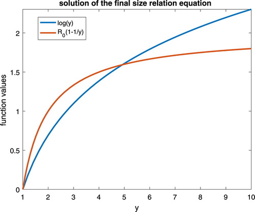Under the condition of ${\mathcal{R}}_0>1$, the population size N is large and the initial size of infectious cases is small, the final epidemic size has been well studied in many publications (e.g. [9,14]) and can be expressed in the following implicit equation: (4) $\log \frac{N}{S_{\mathrm{\infty }}}={\mathcal{R}}_0(1-\frac{S_{\mathrm{\infty }}}{N}).$(4) Once the basic reproduction number $R_0$ is estimated, the final epidemic size can be approximated by Equation (4(4) $\log \frac{N}{S_{\mathrm{\infty }}}={\mathcal{R}}_0(1-\frac{S_{\mathrm{\infty }}}{N}).$(4) ). It can be observed in Equation (4(4) $\log \frac{N}{S_{\mathrm{\infty }}}={\mathcal{R}}_0(1-\frac{S_{\mathrm{\infty }}}{N}).$(4) ) that the final size is solely determined by the value of ${\mathcal{R}}_0$. Furthermore, $S_{\mathrm{\infty }}$ in Equation (4(4) $\log \frac{N}{S_{\mathrm{\infty }}}={\mathcal{R}}_0(1-\frac{S_{\mathrm{\infty }}}{N}).$(4) ) is uniquely determined by ${\mathcal{R}}_0$ and the estimation of its upper bound is available. The final epidemic size can be expressed as a monotonically increasing function of ${\mathcal{R}}_0$. With the larger value of ${\mathcal{R}}_0$, the predicted final epidemic size is larger. The following two lemmas summarize the results.

Lemma 2.1

$S_{\mathrm{\infty }}$ in Equation (4(4) $\log \frac{N}{S_{\mathrm{\infty }}}={\mathcal{R}}_0(1-\frac{S_{\mathrm{\infty }}}{N}).$(4) ) is uniquely determined by the value of ${\mathcal{R}}_0$, and has upper bound of $\frac{N}{{\mathcal{R}}_0}$.

Proof.

We denote $y:=\frac{N}{S_{\mathrm{\infty }}}$, then the left-hand side of Equation (4(4) $\log \frac{N}{S_{\mathrm{\infty }}}={\mathcal{R}}_0(1-\frac{S_{\mathrm{\infty }}}{N}).$(4) ) is denoted by $f_1(y):=\log (y)$, the right-hand side of (4(4) $\log \frac{N}{S_{\mathrm{\infty }}}={\mathcal{R}}_0(1-\frac{S_{\mathrm{\infty }}}{N}).$(4) ) is denoted by $f_2(y):={\mathcal{R}}_0(1-1/y)$. For any fixed ${\mathcal{R}}_0>1$, we analyse the Equation (4(4) $\log \frac{N}{S_{\mathrm{\infty }}}={\mathcal{R}}_0(1-\frac{S_{\mathrm{\infty }}}{N}).$(4) ) step by step:

1. $f_1(1)=0$ and $f_2(1)=0$,

2. $f_1(\mathrm{\infty })=\mathrm{\infty }$ and $f_2(\mathrm{\infty })={\mathcal{R}}_0$,

3. $f_1^{\prime }(y)=1/y$ and $f_2^{\mathrm{\prime }}(y)={\mathcal{R}}_0/y^2$. Both functions $f_1$ and $f_2$ are monotonically increasing functions of y. And we have that if $y\in (1,{\mathcal{R}}_0)$, $f_1^{\prime }(y)<f_2^{\prime }(y)$; while if $y\in ({\mathcal{R}}_0,\mathrm{\infty })$, $f_1^{\prime }(y)>f_2^{\prime }(y)$. If we start from y = 1, the increase of function $f_1$ is slower than the increase of function $f_2$; and starting from $y\ge {\mathcal{R}}_0$, $f_1$ increases faster than $f_2$.

Based on the properties of functions $f_1$ and $f_2$, there exists one and only one solution of Equation (4(4) $\log \frac{N}{S_{\mathrm{\infty }}}={\mathcal{R}}_0(1-\frac{S_{\mathrm{\infty }}}{N}).$(4) ), and $y=\frac{N}{S_{\mathrm{\infty }}}>{\mathcal{R}}_0$. Thus, $S_{\mathrm{\infty }}<\frac{N}{{\mathcal{R}}_0}$. For the case of ${\mathcal{R}}_0<1$, it is clear that two curves generated by $f_1$ and $f_2$ have no intersection for y>1. Only solution for such equation is that y = 1, which indicates there is no outbreak. Because of the linearity between the final size and $S_{\mathrm{\infty }}$, it is straightforward that the final size is uniquely determined by the value of ${\mathcal{R}}_0$ as well. The following Figure 1 shows the case of ${\mathcal{R}}_0=2$.

Figure 1. The uniqueness of the final epidemic size, with respect to the basic reproduction number ${\mathcal{R}}_0$.

Lemma 2.2

As ${\mathcal{R}}_0>1$ increases, $S_{\mathrm{\infty }}$ in (4(4) $\log \frac{N}{S_{\mathrm{\infty }}}={\mathcal{R}}_0(1-\frac{S_{\mathrm{\infty }}}{N}).$(4) ) decreases and the final epidemic size increases.

Proof.

It can be easily proved by considering $S_{\mathrm{\infty }}$ as a function about ${\mathcal{R}}_0$ and differentiate both sides of Equation (4(4) $\log \frac{N}{S_{\mathrm{\infty }}}={\mathcal{R}}_0(1-\frac{S_{\mathrm{\infty }}}{N}).$(4) ) with respect to ${\mathcal{R}}_0$. We have $(\frac{{\mathcal{R}}_0}{N}-\frac{1}{S_{\mathrm{\infty }}})S_{\mathrm{\infty }}^{\mathrm{\prime }}=1-\frac{S_{\mathrm{\infty }}}{N}.$Since we have $1-\frac{S_{\mathrm{\infty }}}{N}>0$ and $\frac{{\mathcal{R}}_0}{N}-\frac{1}{S_{\mathrm{\infty }}}<0$ from the previous lemma, we have $S_{\mathrm{\infty }}^{\prime }<0$. This result is reasonable, because if ${\mathcal{R}}_0$ is larger and the underlying disease is more contagious, the transmission of the epidemic will leave less individuals untouched eventually. The epidemic model predicts a larger final size.

2.2. The epidemic model with behavioural response

We modify model (3(3) $\begin{array}{l}{S}^{\mathrm{\prime }}=-\beta S{\displaystyle \frac{I}{N}},\\ I^{\mathrm{\prime }}=\beta S{\displaystyle \frac{I}{N}}-\gamma I,\\ R^{\mathrm{\prime }}=\gamma I.\end{array}$(3) ) by considering the time-dependent contact rate function (5) $a(t):=\beta ((1-\varphi ){\mathrm{e}}^{-\kappa t}+\varphi )$(5) with $\kappa >0$ (see [18] for more details). β represents the initial contact rate. $a(t)$ is bounded by the initial contact rate $a(0)$ and the eventual contact rate $a(\mathrm{\infty })$, (6) $\beta =a(0)\ge a(t)\ge a(\mathrm{\infty })=\varphi \beta .$(6)

In papers [12,13], the behavioural response function is set to have the form $\beta {\mathrm{e}}^{-\kappa t}$. This is a special case by assuming that, under the circumstance of extremely dangerous infectious diseases, the final contact rate in the population will approach 0 as all individuals tend to avoid any type of contact with others. All other parameters in model (7(7) $\begin{array}{rl}{S}^{\mathrm{\prime }}& =-a(t)S{\displaystyle \frac{I}{N}},\\ I^{\mathrm{\prime }}& =a(t)S{\displaystyle \frac{I}{N}}-\gamma I,\\ R^{\mathrm{\prime }}& =\gamma I.\end{array}$(7) ) are following the assumptions for the SIR epidemic model (3(3) $\begin{array}{l}{S}^{\mathrm{\prime }}=-\beta S{\displaystyle \frac{I}{N}},\\ I^{\mathrm{\prime }}=\beta S{\displaystyle \frac{I}{N}}-\gamma I,\\ R^{\mathrm{\prime }}=\gamma I.\end{array}$(3) ). (7) $\begin{array}{rl}{S}^{\mathrm{\prime }}& =-a(t)S{\displaystyle \frac{I}{N}},\\ I^{\mathrm{\prime }}& =a(t)S{\displaystyle \frac{I}{N}}-\gamma I,\\ R^{\mathrm{\prime }}& =\gamma I.\end{array}$(7) The basic reproduction number ${\mathcal{R}}_0=\frac{\beta }{\gamma }$ of model (7(7) $\begin{array}{rl}{S}^{\mathrm{\prime }}& =-a(t)S{\displaystyle \frac{I}{N}},\\ I^{\mathrm{\prime }}& =a(t)S{\displaystyle \frac{I}{N}}-\gamma I,\\ R^{\mathrm{\prime }}& =\gamma I.\end{array}$(7) ) has the same value as ${\mathcal{R}}_0$ of model (3(3) $\begin{array}{l}{S}^{\mathrm{\prime }}=-\beta S{\displaystyle \frac{I}{N}},\\ I^{\mathrm{\prime }}=\beta S{\displaystyle \frac{I}{N}}-\gamma I,\\ R^{\mathrm{\prime }}=\gamma I.\end{array}$(3) ). Because model (7(7) $\begin{array}{rl}{S}^{\mathrm{\prime }}& =-a(t)S{\displaystyle \frac{I}{N}},\\ I^{\mathrm{\prime }}& =a(t)S{\displaystyle \frac{I}{N}}-\gamma I,\\ R^{\mathrm{\prime }}& =\gamma I.\end{array}$(7) ) is non-autonomous, the explicit formulation of final size relation is impossible to obtain (see [12]). However, we are able to obtain the following result of comparison.

Theorem 2.1

Under the condition of ${\mathcal{R}}_0>1$, the final epidemic size for model (7(7) $\begin{array}{rl}{S}^{\mathrm{\prime }}& =-a(t)S{\displaystyle \frac{I}{N}},\\ I^{\mathrm{\prime }}& =a(t)S{\displaystyle \frac{I}{N}}-\gamma I,\\ R^{\mathrm{\prime }}& =\gamma I.\end{array}$(7) ) is no greater than the final epidemic size for model (3(3) $\begin{array}{l}{S}^{\mathrm{\prime }}=-\beta S{\displaystyle \frac{I}{N}},\\ I^{\mathrm{\prime }}=\beta S{\displaystyle \frac{I}{N}}-\gamma I,\\ R^{\mathrm{\prime }}=\gamma I.\end{array}$(3) ).

Proof.

First, we have $a(t)\le \beta$ for $0\le t<\mathrm{\infty }$. To distinguish populations for two models (3(3) $\begin{array}{l}{S}^{\mathrm{\prime }}=-\beta S{\displaystyle \frac{I}{N}},\\ I^{\mathrm{\prime }}=\beta S{\displaystyle \frac{I}{N}}-\gamma I,\\ R^{\mathrm{\prime }}=\gamma I.\end{array}$(3) ) and (7(7) $\begin{array}{rl}{S}^{\mathrm{\prime }}& =-a(t)S{\displaystyle \frac{I}{N}},\\ I^{\mathrm{\prime }}& =a(t)S{\displaystyle \frac{I}{N}}-\gamma I,\\ R^{\mathrm{\prime }}& =\gamma I.\end{array}$(7) ), we use the subscripts 1 and 2 for model (3(3) $\begin{array}{l}{S}^{\mathrm{\prime }}=-\beta S{\displaystyle \frac{I}{N}},\\ I^{\mathrm{\prime }}=\beta S{\displaystyle \frac{I}{N}}-\gamma I,\\ R^{\mathrm{\prime }}=\gamma I.\end{array}$(3) ) and model (7(7) $\begin{array}{rl}{S}^{\mathrm{\prime }}& =-a(t)S{\displaystyle \frac{I}{N}},\\ I^{\mathrm{\prime }}& =a(t)S{\displaystyle \frac{I}{N}}-\gamma I,\\ R^{\mathrm{\prime }}& =\gamma I.\end{array}$(7) ), respectively. Addition of the first two equations of model (3(3) $\begin{array}{l}{S}^{\mathrm{\prime }}=-\beta S{\displaystyle \frac{I}{N}},\\ I^{\mathrm{\prime }}=\beta S{\displaystyle \frac{I}{N}}-\gamma I,\\ R^{\mathrm{\prime }}=\gamma I.\end{array}$(3) ) gives $[S_1(t)+I_1(t){]}^{\mathrm{\prime }}=-\gamma I_1(t),$and the integration indicates that (8) $N-S_1(\mathrm{\infty })=\gamma {\int }_0^{\mathrm{\infty }}{I}_1(t)\mathrm{d}t.$(8) Similarly, for model (7(7) $\begin{array}{rl}{S}^{\mathrm{\prime }}& =-a(t)S{\displaystyle \frac{I}{N}},\\ I^{\mathrm{\prime }}& =a(t)S{\displaystyle \frac{I}{N}}-\gamma I,\\ R^{\mathrm{\prime }}& =\gamma I.\end{array}$(7) ), (9) $N-S_2(\mathrm{\infty })=\gamma {\int }_0^{\mathrm{\infty }}{I}_2(t)\mathrm{d}t.$(9) Integration of first equations of model (3(3) $\begin{array}{l}{S}^{\mathrm{\prime }}=-\beta S{\displaystyle \frac{I}{N}},\\ I^{\mathrm{\prime }}=\beta S{\displaystyle \frac{I}{N}}-\gamma I,\\ R^{\mathrm{\prime }}=\gamma I.\end{array}$(3) ) and model (7(7) $\begin{array}{rl}{S}^{\mathrm{\prime }}& =-a(t)S{\displaystyle \frac{I}{N}},\\ I^{\mathrm{\prime }}& =a(t)S{\displaystyle \frac{I}{N}}-\gamma I,\\ R^{\mathrm{\prime }}& =\gamma I.\end{array}$(7) ) gives (10) $\begin{array}{rl}\log \frac{N}{S_1(\mathrm{\infty })}& =\frac{\beta }{\gamma }[1-\frac{S_1(\mathrm{\infty })}{N}],\\ \log \frac{N}{S_2(\mathrm{\infty })}& ={\displaystyle \frac{{\int }_0^{\mathrm{\infty }}a(t)I_2(t)\mathrm{d}t}{N}\le \frac{\beta }{\gamma }[1-\frac{S_2(\mathrm{\infty })}{N}].}\end{array}$(10) Since $\log \frac{N}{x}$ is a monotonic decreasing function of x, this implies $S_2(\mathrm{\infty })\ge S_1(\mathrm{\infty }).$We further have $N-S_2(\mathrm{\infty })\le N-S_1(\mathrm{\infty }),$as desired.

2.3. The epidemic model with heterogeneous mixing

As mentioned in [12,13,18], another explanation for the smaller epidemic final size than expected is the heterogeneous mixing of the population. One typical way to consider the heterogeneous mixing is to assume that the population can be divided into two sub-populations based on different activity levels, one is with size $N_1$ and the other one is with size $N_2$ (see [10]). We assume that individuals in group i make ${\beta }_i$ contacts in unit time and then define $p_{ij}$ the probability that one contact made by an individual of group i that is with an individual of group j, for i, j = 1, 2. We have $p_{11}+p_{12}=p_{21}+p_{22}=1,$and the balance relation equation (11) $p_{21}{\beta }_2{N}_2=p_{12}{\beta }_1{N}_1.$(11) We assume that the recover rates for both sub-populations are equal, which suggests that the only source of heterogeneity is the different activity levels. Similar with assumptions made in [10,12,13], we set ${\beta }_1>{\beta }_2$, which indicates that sub-population 1 is more active than sub-population 2. Sub-population 1 can be treated as the group of superspreaders who are responsible for the majority of transmissions.

The epidemic model with two sub-populations is (12) $\begin{array}{rl}{S}_1^{\mathrm{\prime }}& =-S_1[p_{11}{\beta }_1{\displaystyle \frac{I_1}{N_1}}+p_{12}{\beta }_1{\displaystyle \frac{I_2}{N_2}}],\\ I_1^{\mathrm{\prime }}& =S_1[p_{11}{\beta }_1{\displaystyle \frac{I_1}{N_1}}+p_{12}{\beta }_1{\displaystyle \frac{I_2}{N_2}}]-\gamma I_1,\\ R_1^{\mathrm{\prime }}& =\gamma I_1,\\ S_2^{\mathrm{\prime }}& =-S_2[p_{21}{\beta }_2{\displaystyle \frac{I_1}{N_1}}+p_{22}{\beta }_2{\displaystyle \frac{I_2}{N_2}}],\\ I_2^{\mathrm{\prime }}& =S_2[p_{21}{\beta }_2{\displaystyle \frac{I_1}{N_1}}+p_{22}{\beta }_2{\displaystyle \frac{I_2}{N_2}}]-\gamma I_2,\\ R_2^{\mathrm{\prime }}& =\gamma I_2.\end{array}$(12) By using the next generation matrix approach (described in [20]), the basic reproduction number can be expressed as ${\mathcal{R}}_0=\frac{1}{2}(\frac{p_{11}{\beta }_1+p_{22}{\beta }_2}{\gamma }+\frac{\sqrt{(p_{11}{\beta }_1-p_{22}{\beta }_2{)}^2+4p_{12}{p}_{21}{\beta }_1{\beta }_2}}{\gamma }).$As discussed in [10], it is necessary to make some assumptions about the nature of mixing between two sub-populations in order to obtain more useful expression. One reasonable assumption is the proportional mixing, which suggests that mixing is random but constrained by the activity level. Thus, we assume (13) $p_{ij}=\frac{{\beta }_j{N}_j}{{\beta }_1{N}_1+{\beta }_2{N}_2},i,j=1,2.$(13) Then we have $p_{11}=p_{21}=:p_1$ and $p_{12}=p_{22}=:p_2$. Furthermore, the basic reproduction number ${\mathcal{R}}_0$ is (14) ${\mathcal{R}}_0=\frac{p_1{\beta }_1+p_2{\beta }_2}{\gamma }.$(14)

We explain the formula of ${\mathcal{R}}_0$ in Equation (14(14) ${\mathcal{R}}_0=\frac{p_1{\beta }_1+p_2{\beta }_2}{\gamma }.$(14) ) in the following way: suppose that the disease is initiated by an infectious outsider. Then with the probability of $p_1$, the outsider contacts a susceptible individual in sub-population 1, and with the probability of $p_2$, this outsider will contact with a susceptible individual in sub-population 2. Thus, the first infectious case of the wholly susceptible population will appear in sub-population 1 with probability $p_1$ and will appear in sub-population 2 with probability $p_2$. If the first infectious individual belongs to the sub-population 1, the number of secondary infectious cases is ${\beta }_1/\gamma$, while if the first infectious individual belongs to sub-population 2, the number of the secondary infectious cases is ${\beta }_2/\gamma$. So the number of total secondary infectious cases by introducing one infectious individual is $\frac{p_1{\beta }_1+p_2{\beta }_2}{\gamma }$.

For the rest of this paper, we use the notations $p_1$ and $p_2$ to replace the parameters $p_{11}$, $p_{12}$, $p_{21}$ and $p_{22}$ in model (12(12) $\begin{array}{rl}{S}_1^{\mathrm{\prime }}& =-S_1[p_{11}{\beta }_1{\displaystyle \frac{I_1}{N_1}}+p_{12}{\beta }_1{\displaystyle \frac{I_2}{N_2}}],\\ I_1^{\mathrm{\prime }}& =S_1[p_{11}{\beta }_1{\displaystyle \frac{I_1}{N_1}}+p_{12}{\beta }_1{\displaystyle \frac{I_2}{N_2}}]-\gamma I_1,\\ R_1^{\mathrm{\prime }}& =\gamma I_1,\\ S_2^{\mathrm{\prime }}& =-S_2[p_{21}{\beta }_2{\displaystyle \frac{I_1}{N_1}}+p_{22}{\beta }_2{\displaystyle \frac{I_2}{N_2}}],\\ I_2^{\mathrm{\prime }}& =S_2[p_{21}{\beta }_2{\displaystyle \frac{I_1}{N_1}}+p_{22}{\beta }_2{\displaystyle \frac{I_2}{N_2}}]-\gamma I_2,\\ R_2^{\mathrm{\prime }}& =\gamma I_2.\end{array}$(12) ). As mentioned in [12,13], in order to guarantee that the basic reproduction number ${\mathcal{R}}_0$ in (14(14) ${\mathcal{R}}_0=\frac{p_1{\beta }_1+p_2{\beta }_2}{\gamma }.$(14) ) for model (12(12) $\begin{array}{rl}{S}_1^{\mathrm{\prime }}& =-S_1[p_{11}{\beta }_1{\displaystyle \frac{I_1}{N_1}}+p_{12}{\beta }_1{\displaystyle \frac{I_2}{N_2}}],\\ I_1^{\mathrm{\prime }}& =S_1[p_{11}{\beta }_1{\displaystyle \frac{I_1}{N_1}}+p_{12}{\beta }_1{\displaystyle \frac{I_2}{N_2}}]-\gamma I_1,\\ R_1^{\mathrm{\prime }}& =\gamma I_1,\\ S_2^{\mathrm{\prime }}& =-S_2[p_{21}{\beta }_2{\displaystyle \frac{I_1}{N_1}}+p_{22}{\beta }_2{\displaystyle \frac{I_2}{N_2}}],\\ I_2^{\mathrm{\prime }}& =S_2[p_{21}{\beta }_2{\displaystyle \frac{I_1}{N_1}}+p_{22}{\beta }_2{\displaystyle \frac{I_2}{N_2}}]-\gamma I_2,\\ R_2^{\mathrm{\prime }}& =\gamma I_2.\end{array}$(12) ) has the same value as the model (3(3) $\begin{array}{l}{S}^{\mathrm{\prime }}=-\beta S{\displaystyle \frac{I}{N}},\\ I^{\mathrm{\prime }}=\beta S{\displaystyle \frac{I}{N}}-\gamma I,\\ R^{\mathrm{\prime }}=\gamma I.\end{array}$(3) ) with homogeneous mixing, we need to make (15) $\beta =p_1{\beta }_1+p_2{\beta }_2,$(15) which implies that the contact rate β for the homogeneous-mixing model (3(3) $\begin{array}{l}{S}^{\mathrm{\prime }}=-\beta S{\displaystyle \frac{I}{N}},\\ I^{\mathrm{\prime }}=\beta S{\displaystyle \frac{I}{N}}-\gamma I,\\ R^{\mathrm{\prime }}=\gamma I.\end{array}$(3) ) is the weighted average of contact rates ${\beta }_1$ and ${\beta }_2$. Assume that the average contact rate β is estimated from the epidemiological data, then what are the actual activity levels for the group of superspreaders and for the group of non-superspreaders? To answer this question, we first denote $k=\frac{N_2}{N_1}$ representing the ratio between the group size of the non-superspreaders and the group size of the superspreaders. Then we assume that ${\beta }_1=c_1\beta$ with $c_1>1$ and ${\beta }_2=c_2\beta$ with $c_2<1$. $c_1$ and $c_2$ account for the scaled activity levels for each group. Thus, we are able to express the proportion of transmissions due to the group of the superspreaders $\frac{c_1}{c_1+k{c}_2}$.

Moreover, formula (15(15) $\beta =p_1{\beta }_1+p_2{\beta }_2,$(15) ) leads to the equation (16) $c_1(c_1-1)=k{c}_2(1-c_2).$(16) Since we have $c_2\in (0,1)$, it is straightforward to have $k{c}_2(1-c_2)\in (0,\frac{k}{4})$ with the critical point $c_2=\frac{1}{2}$. This indicates the upper bound for $c_1$ (17) $max\{c_1\}=\frac{1+\sqrt{1+k}}{2}.$(17) The final size relation for model (12(12) $\begin{array}{rl}{S}_1^{\mathrm{\prime }}& =-S_1[p_{11}{\beta }_1{\displaystyle \frac{I_1}{N_1}}+p_{12}{\beta }_1{\displaystyle \frac{I_2}{N_2}}],\\ I_1^{\mathrm{\prime }}& =S_1[p_{11}{\beta }_1{\displaystyle \frac{I_1}{N_1}}+p_{12}{\beta }_1{\displaystyle \frac{I_2}{N_2}}]-\gamma I_1,\\ R_1^{\mathrm{\prime }}& =\gamma I_1,\\ S_2^{\mathrm{\prime }}& =-S_2[p_{21}{\beta }_2{\displaystyle \frac{I_1}{N_1}}+p_{22}{\beta }_2{\displaystyle \frac{I_2}{N_2}}],\\ I_2^{\mathrm{\prime }}& =S_2[p_{21}{\beta }_2{\displaystyle \frac{I_1}{N_1}}+p_{22}{\beta }_2{\displaystyle \frac{I_2}{N_2}}]-\gamma I_2,\\ R_2^{\mathrm{\prime }}& =\gamma I_2.\end{array}$(12) ) with heterogeneous mixing can be expressed as the following system of equations (see [10]): (18) $\begin{array}{rl}\log \frac{N_1}{S_1(\mathrm{\infty })}& =\frac{p_1{\beta }_1}{\gamma }\frac{N_1-S_1(\mathrm{\infty })}{N_1}+\frac{p_2{\beta }_1}{\gamma }\frac{N_2-S_2(\mathrm{\infty })}{N_2},\\ \log \frac{N_2}{S_2(\mathrm{\infty })}& =\frac{p_1{\beta }_2}{\gamma }\frac{N_1-S_1(\mathrm{\infty })}{N_1}+\frac{p_2{\beta }_2}{\gamma }\frac{N_2-S_2(\mathrm{\infty })}{N_2}.\end{array}$(18) The above final size relation (18(18) $\begin{array}{rl}\log \frac{N_1}{S_1(\mathrm{\infty })}& =\frac{p_1{\beta }_1}{\gamma }\frac{N_1-S_1(\mathrm{\infty })}{N_1}+\frac{p_2{\beta }_1}{\gamma }\frac{N_2-S_2(\mathrm{\infty })}{N_2},\\ \log \frac{N_2}{S_2(\mathrm{\infty })}& =\frac{p_1{\beta }_2}{\gamma }\frac{N_1-S_1(\mathrm{\infty })}{N_1}+\frac{p_2{\beta }_2}{\gamma }\frac{N_2-S_2(\mathrm{\infty })}{N_2}.\end{array}$(18) ) for the epidemic model with multiple sub-groups has been studied in several papers, such as [4,10,12,13,28,29]. However, if the basic reproduction numbers ${\mathcal{R}}_0$ for model (12(12) $\begin{array}{rl}{S}_1^{\mathrm{\prime }}& =-S_1[p_{11}{\beta }_1{\displaystyle \frac{I_1}{N_1}}+p_{12}{\beta }_1{\displaystyle \frac{I_2}{N_2}}],\\ I_1^{\mathrm{\prime }}& =S_1[p_{11}{\beta }_1{\displaystyle \frac{I_1}{N_1}}+p_{12}{\beta }_1{\displaystyle \frac{I_2}{N_2}}]-\gamma I_1,\\ R_1^{\mathrm{\prime }}& =\gamma I_1,\\ S_2^{\mathrm{\prime }}& =-S_2[p_{21}{\beta }_2{\displaystyle \frac{I_1}{N_1}}+p_{22}{\beta }_2{\displaystyle \frac{I_2}{N_2}}],\\ I_2^{\mathrm{\prime }}& =S_2[p_{21}{\beta }_2{\displaystyle \frac{I_1}{N_1}}+p_{22}{\beta }_2{\displaystyle \frac{I_2}{N_2}}]-\gamma I_2,\\ R_2^{\mathrm{\prime }}& =\gamma I_2.\end{array}$(12) ) and model (7(7) $\begin{array}{rl}{S}^{\mathrm{\prime }}& =-a(t)S{\displaystyle \frac{I}{N}},\\ I^{\mathrm{\prime }}& =a(t)S{\displaystyle \frac{I}{N}}-\gamma I,\\ R^{\mathrm{\prime }}& =\gamma I.\end{array}$(7) ) are set to be identical, what is the relation between the final epidemic size $N-(S_1(\mathrm{\infty })+S_2(\mathrm{\infty }))$ in Equation (18(18) $\begin{array}{rl}\log \frac{N_1}{S_1(\mathrm{\infty })}& =\frac{p_1{\beta }_1}{\gamma }\frac{N_1-S_1(\mathrm{\infty })}{N_1}+\frac{p_2{\beta }_1}{\gamma }\frac{N_2-S_2(\mathrm{\infty })}{N_2},\\ \log \frac{N_2}{S_2(\mathrm{\infty })}& =\frac{p_1{\beta }_2}{\gamma }\frac{N_1-S_1(\mathrm{\infty })}{N_1}+\frac{p_2{\beta }_2}{\gamma }\frac{N_2-S_2(\mathrm{\infty })}{N_2}.\end{array}$(18) ) and the final size $N-S_{\mathrm{\infty }}$ in Equation (4(4) $\log \frac{N}{S_{\mathrm{\infty }}}={\mathcal{R}}_0(1-\frac{S_{\mathrm{\infty }}}{N}).$(4) )? Will the epidemic model with homogeneous mixing always predict the worst result with the largest final epidemic size?

To compare the value of $S_{\mathrm{\infty }}$ and the value of $S_1(\mathrm{\infty })+S_2(\mathrm{\infty })$, we first focus on Equation (18(18) $\begin{array}{rl}\log \frac{N_1}{S_1(\mathrm{\infty })}& =\frac{p_1{\beta }_1}{\gamma }\frac{N_1-S_1(\mathrm{\infty })}{N_1}+\frac{p_2{\beta }_1}{\gamma }\frac{N_2-S_2(\mathrm{\infty })}{N_2},\\ \log \frac{N_2}{S_2(\mathrm{\infty })}& =\frac{p_1{\beta }_2}{\gamma }\frac{N_1-S_1(\mathrm{\infty })}{N_1}+\frac{p_2{\beta }_2}{\gamma }\frac{N_2-S_2(\mathrm{\infty })}{N_2}.\end{array}$(18) ). Simple calculations lead to $\log \frac{N_1}{S_1(\mathrm{\infty })}/\log \frac{N_2}{S_2(\mathrm{\infty })}=\frac{{\beta }_1}{{\beta }_2}.$We further have ${\left(\frac{S_1(\mathrm{\infty })}{N_1}\right)}^{{\beta }_2}={\left(\frac{S_2(\mathrm{\infty })}{N_2}\right)}^{{\beta }_1}.$As the assumption is that $N_1$ represents the group of superspreaders, we have $N_1\ll N_2$ and ${\beta }_1\gg {\beta }_2$. If we denote $\sigma :=\frac{{\beta }_1}{{\beta }_2}\gg 1$, the above equation becomes $\frac{S_1(\mathrm{\infty })}{N_1}={\left(\frac{S_2(\mathrm{\infty })}{N_2}\right)}^{\sigma }.$For a relatively large value of σ, no matter what value $\frac{S_1(\mathrm{\infty })}{N_1}$ is, the value of $\frac{S_2(\mathrm{\infty })}{N_2}$ cannot be much smaller than 1. In other words, the group of non-superspreaders is less affected by the epidemic. Considering that the size of the group of non-superspreaders is relatively large, the overall population is less affected. Thus, we conclude that the total final size is smaller than predicted by the model with homogeneous mixing. For the larger σ, the discrepancy between predictions of both models with homogeneous mixing and heterogeneous mixing is more obvious. To support the statement, many combinations of parameter values ${\beta }_1$, ${\beta }_2$, $N_1$ and $N_2$ are tested in the subsection of numerical experiments. We use the following theorem to summarize our study. However, the detailed analytical (algebraic) proof for this conjecture remains for future work.

Conjecture 2.1

For epidemic models with the identical value of basic reproduction number ${\mathcal{R}}_0$, the final size for the epidemic model with homogeneous mixing is larger or equal to the final size of the epidemic model with heterogeneous mixing.

Following the study of final size relations in papers [12,13], we investigate more of this subject in Section 2.5 from the point view of numerical simulations. Several combinations of heterogeneous mixing parameters are studied to numerically test the above conjecture.

2.4. The epidemic model with behavioural changes and heterogeneity

(19) $\begin{array}{rl}{S}_1^{\mathrm{\prime }}& =-S_1{a}_1(t)[p_1{\displaystyle \frac{I_1}{N_1}}+p_2{\displaystyle \frac{I_2}{N_2}}],\\ I_1^{\mathrm{\prime }}& =S_1{a}_1(t)[p_1{\displaystyle \frac{I_1}{N_1}}+p_2{\displaystyle \frac{I_2}{N_2}}]-\gamma I_1,\\ R_1^{\mathrm{\prime }}& =\gamma I_1,\\ S_2^{\mathrm{\prime }}& =-S_2{a}_2(t)[p_1{\displaystyle \frac{I_1}{N_1}}+p_2{\displaystyle \frac{I_2}{N_2}}],\\ I_2^{\mathrm{\prime }}& =S_2{a}_2(t)[p_1{\displaystyle \frac{I_1}{N_1}}+p_2{\displaystyle \frac{I_2}{N_2}}]-\gamma I_2,\\ R_2^{\mathrm{\prime }}& =\gamma I_2.\end{array}$(19) The model is modified by considering two behavioural response functions $a_1(t)$ and $a_2(t)$, both functions are monotonically decreasing functions and have the expressions (20) $\begin{array}{rl}{a}_1(t)& :={\beta }_1((1-{\varphi }_1){\mathrm{e}}^{-{\kappa }_{1}t}+{\varphi }_1),\\ a_2(t)& :={\beta }_2((1-{\varphi }_2){\mathrm{e}}^{-{\kappa }_{2}t}+{\varphi }_2).\end{array}$(20) The initial contact rates ${\beta }_1$ and ${\beta }_2$ are varied and the decreasing rates ${\kappa }_{1,2}$ for both sub-groups have different values as well. For sub-group with the faster response, the value of the decreasing rate is larger. The final contact rates are determined by the values of ${\varphi }_1$ and ${\varphi }_2$. For model (19(19) $\begin{array}{rl}{S}_1^{\mathrm{\prime }}& =-S_1{a}_1(t)[p_1{\displaystyle \frac{I_1}{N_1}}+p_2{\displaystyle \frac{I_2}{N_2}}],\\ I_1^{\mathrm{\prime }}& =S_1{a}_1(t)[p_1{\displaystyle \frac{I_1}{N_1}}+p_2{\displaystyle \frac{I_2}{N_2}}]-\gamma I_1,\\ R_1^{\mathrm{\prime }}& =\gamma I_1,\\ S_2^{\mathrm{\prime }}& =-S_2{a}_2(t)[p_1{\displaystyle \frac{I_1}{N_1}}+p_2{\displaystyle \frac{I_2}{N_2}}],\\ I_2^{\mathrm{\prime }}& =S_2{a}_2(t)[p_1{\displaystyle \frac{I_1}{N_1}}+p_2{\displaystyle \frac{I_2}{N_2}}]-\gamma I_2,\\ R_2^{\mathrm{\prime }}& =\gamma I_2.\end{array}$(19) ), the basic reproduction number ${\mathcal{R}}_0$ has the same value comparing as model (12(12) $\begin{array}{rl}{S}_1^{\mathrm{\prime }}& =-S_1[p_{11}{\beta }_1{\displaystyle \frac{I_1}{N_1}}+p_{12}{\beta }_1{\displaystyle \frac{I_2}{N_2}}],\\ I_1^{\mathrm{\prime }}& =S_1[p_{11}{\beta }_1{\displaystyle \frac{I_1}{N_1}}+p_{12}{\beta }_1{\displaystyle \frac{I_2}{N_2}}]-\gamma I_1,\\ R_1^{\mathrm{\prime }}& =\gamma I_1,\\ S_2^{\mathrm{\prime }}& =-S_2[p_{21}{\beta }_2{\displaystyle \frac{I_1}{N_1}}+p_{22}{\beta }_2{\displaystyle \frac{I_2}{N_2}}],\\ I_2^{\mathrm{\prime }}& =S_2[p_{21}{\beta }_2{\displaystyle \frac{I_1}{N_1}}+p_{22}{\beta }_2{\displaystyle \frac{I_2}{N_2}}]-\gamma I_2,\\ R_2^{\mathrm{\prime }}& =\gamma I_2.\end{array}$(12) ). Because the model is also non-autonomous, the explicit formulation of the final size relation for model (19(19) $\begin{array}{rl}{S}_1^{\mathrm{\prime }}& =-S_1{a}_1(t)[p_1{\displaystyle \frac{I_1}{N_1}}+p_2{\displaystyle \frac{I_2}{N_2}}],\\ I_1^{\mathrm{\prime }}& =S_1{a}_1(t)[p_1{\displaystyle \frac{I_1}{N_1}}+p_2{\displaystyle \frac{I_2}{N_2}}]-\gamma I_1,\\ R_1^{\mathrm{\prime }}& =\gamma I_1,\\ S_2^{\mathrm{\prime }}& =-S_2{a}_2(t)[p_1{\displaystyle \frac{I_1}{N_1}}+p_2{\displaystyle \frac{I_2}{N_2}}],\\ I_2^{\mathrm{\prime }}& =S_2{a}_2(t)[p_1{\displaystyle \frac{I_1}{N_1}}+p_2{\displaystyle \frac{I_2}{N_2}}]-\gamma I_2,\\ R_2^{\mathrm{\prime }}& =\gamma I_2.\end{array}$(19) ) is impossible to obtain. We argue that if the statement in Conjecture 2.1 is correct and considering the analytical results for model (7(7) $\begin{array}{rl}{S}^{\mathrm{\prime }}& =-a(t)S{\displaystyle \frac{I}{N}},\\ I^{\mathrm{\prime }}& =a(t)S{\displaystyle \frac{I}{N}}-\gamma I,\\ R^{\mathrm{\prime }}& =\gamma I.\end{array}$(7) ), then model (19(19) $\begin{array}{rl}{S}_1^{\mathrm{\prime }}& =-S_1{a}_1(t)[p_1{\displaystyle \frac{I_1}{N_1}}+p_2{\displaystyle \frac{I_2}{N_2}}],\\ I_1^{\mathrm{\prime }}& =S_1{a}_1(t)[p_1{\displaystyle \frac{I_1}{N_1}}+p_2{\displaystyle \frac{I_2}{N_2}}]-\gamma I_1,\\ R_1^{\mathrm{\prime }}& =\gamma I_1,\\ S_2^{\mathrm{\prime }}& =-S_2{a}_2(t)[p_1{\displaystyle \frac{I_1}{N_1}}+p_2{\displaystyle \frac{I_2}{N_2}}],\\ I_2^{\mathrm{\prime }}& =S_2{a}_2(t)[p_1{\displaystyle \frac{I_1}{N_1}}+p_2{\displaystyle \frac{I_2}{N_2}}]-\gamma I_2,\\ R_2^{\mathrm{\prime }}& =\gamma I_2.\end{array}$(19) ) should predict the smallest final epidemic size.

2.5. Numerical simulations on deterministic models

2.5.1. Numerical simulation 1

We now perform several numerical experiments to compare the final sizes predicted by different epidemic models which have been discussed, most of the parameter values are taken from [13]. The size of the population under study is N = 5000. It is also possible to test for cases with larger population sizes (see [12,13]). The recovery rate $\gamma =\frac{1}{5.61}$. For model (3(3) $\begin{array}{l}{S}^{\mathrm{\prime }}=-\beta S{\displaystyle \frac{I}{N}},\\ I^{\mathrm{\prime }}=\beta S{\displaystyle \frac{I}{N}}-\gamma I,\\ R^{\mathrm{\prime }}=\gamma I.\end{array}$(3) ), the contact rate $\beta =0.27$, which is also the initial contact rate for model (7(7) $\begin{array}{rl}{S}^{\mathrm{\prime }}& =-a(t)S{\displaystyle \frac{I}{N}},\\ I^{\mathrm{\prime }}& =a(t)S{\displaystyle \frac{I}{N}}-\gamma I,\\ R^{\mathrm{\prime }}& =\gamma I.\end{array}$(7) ). For model (7(7) $\begin{array}{rl}{S}^{\mathrm{\prime }}& =-a(t)S{\displaystyle \frac{I}{N}},\\ I^{\mathrm{\prime }}& =a(t)S{\displaystyle \frac{I}{N}}-\gamma I,\\ R^{\mathrm{\prime }}& =\gamma I.\end{array}$(7) ), we set $\varphi =0$ and the decreasing rate κ in the response function is 0.0023. For models (12(12) $\begin{array}{rl}{S}_1^{\mathrm{\prime }}& =-S_1[p_{11}{\beta }_1{\displaystyle \frac{I_1}{N_1}}+p_{12}{\beta }_1{\displaystyle \frac{I_2}{N_2}}],\\ I_1^{\mathrm{\prime }}& =S_1[p_{11}{\beta }_1{\displaystyle \frac{I_1}{N_1}}+p_{12}{\beta }_1{\displaystyle \frac{I_2}{N_2}}]-\gamma I_1,\\ R_1^{\mathrm{\prime }}& =\gamma I_1,\\ S_2^{\mathrm{\prime }}& =-S_2[p_{21}{\beta }_2{\displaystyle \frac{I_1}{N_1}}+p_{22}{\beta }_2{\displaystyle \frac{I_2}{N_2}}],\\ I_2^{\mathrm{\prime }}& =S_2[p_{21}{\beta }_2{\displaystyle \frac{I_1}{N_1}}+p_{22}{\beta }_2{\displaystyle \frac{I_2}{N_2}}]-\gamma I_2,\\ R_2^{\mathrm{\prime }}& =\gamma I_2.\end{array}$(12) ) and (19(19) $\begin{array}{rl}{S}_1^{\mathrm{\prime }}& =-S_1{a}_1(t)[p_1{\displaystyle \frac{I_1}{N_1}}+p_2{\displaystyle \frac{I_2}{N_2}}],\\ I_1^{\mathrm{\prime }}& =S_1{a}_1(t)[p_1{\displaystyle \frac{I_1}{N_1}}+p_2{\displaystyle \frac{I_2}{N_2}}]-\gamma I_1,\\ R_1^{\mathrm{\prime }}& =\gamma I_1,\\ S_2^{\mathrm{\prime }}& =-S_2{a}_2(t)[p_1{\displaystyle \frac{I_1}{N_1}}+p_2{\displaystyle \frac{I_2}{N_2}}],\\ I_2^{\mathrm{\prime }}& =S_2{a}_2(t)[p_1{\displaystyle \frac{I_1}{N_1}}+p_2{\displaystyle \frac{I_2}{N_2}}]-\gamma I_2,\\ R_2^{\mathrm{\prime }}& =\gamma I_2.\end{array}$(19) ) with heterogeneous mixing, the population sizes are $N_1=1000$ and $N_2=4000$, respectively. The (initial) contact rates ${\beta }_1=\frac{16}{13}\beta$ and ${\beta }_2=\frac{1}{13}\beta$. By the definition of proportionate mixing, $p_1=0.8$ and $p_2=0.2$ can be calculated. The careful setup is to conform with the 20/80 rule which states that commonly roughly $20\mathrm{\%}$ of the individuals in a population are responsible for $80\mathrm{\%}$ of the disease cases (also discussed in [13,21]). Sub-group 1 is considered as the group of superspreaders. For model (19(19) $\begin{array}{rl}{S}_1^{\mathrm{\prime }}& =-S_1{a}_1(t)[p_1{\displaystyle \frac{I_1}{N_1}}+p_2{\displaystyle \frac{I_2}{N_2}}],\\ I_1^{\mathrm{\prime }}& =S_1{a}_1(t)[p_1{\displaystyle \frac{I_1}{N_1}}+p_2{\displaystyle \frac{I_2}{N_2}}]-\gamma I_1,\\ R_1^{\mathrm{\prime }}& =\gamma I_1,\\ S_2^{\mathrm{\prime }}& =-S_2{a}_2(t)[p_1{\displaystyle \frac{I_1}{N_1}}+p_2{\displaystyle \frac{I_2}{N_2}}],\\ I_2^{\mathrm{\prime }}& =S_2{a}_2(t)[p_1{\displaystyle \frac{I_1}{N_1}}+p_2{\displaystyle \frac{I_2}{N_2}}]-\gamma I_2,\\ R_2^{\mathrm{\prime }}& =\gamma I_2.\end{array}$(19) ), ${\varphi }_1={\varphi }_2=0$ and ${\kappa }_1={\kappa }_2=0.0023$, imply that individuals in both sub-groups have the same response to the epidemic. It is also plausible to assume that two response functions are different. The basic reproduction numbers ${\mathcal{R}}_0$ for all models can be calculated as ${\mathcal{R}}_0=\frac{p_1{\beta }_1+p_2{\beta }_2}{\gamma }=\frac{\beta }{\gamma }=\mathrm{1.5147.}$Figure 2 shows the dynamics of the models. We summarize the values of final sizes for the models in Table 1.

Figure 2. The x-axis represents time (in days) and the y-axis represents the numbers of individuals in different compartments with respect to time. Outbreaks are initiated by one infectious individual. Plots on lower left and on lower right represent the sums of $S_1+S_2$, $I_1+I_2$ and $R_1+R_2$ for models (12(12) $\begin{array}{rl}{S}_1^{\mathrm{\prime }}& =-S_1[p_{11}{\beta }_1{\displaystyle \frac{I_1}{N_1}}+p_{12}{\beta }_1{\displaystyle \frac{I_2}{N_2}}],\\ I_1^{\mathrm{\prime }}& =S_1[p_{11}{\beta }_1{\displaystyle \frac{I_1}{N_1}}+p_{12}{\beta }_1{\displaystyle \frac{I_2}{N_2}}]-\gamma I_1,\\ R_1^{\mathrm{\prime }}& =\gamma I_1,\\ S_2^{\mathrm{\prime }}& =-S_2[p_{21}{\beta }_2{\displaystyle \frac{I_1}{N_1}}+p_{22}{\beta }_2{\displaystyle \frac{I_2}{N_2}}],\\ I_2^{\mathrm{\prime }}& =S_2[p_{21}{\beta }_2{\displaystyle \frac{I_1}{N_1}}+p_{22}{\beta }_2{\displaystyle \frac{I_2}{N_2}}]-\gamma I_2,\\ R_2^{\mathrm{\prime }}& =\gamma I_2.\end{array}$(12) ) and (19(19) $\begin{array}{rl}{S}_1^{\mathrm{\prime }}& =-S_1{a}_1(t)[p_1{\displaystyle \frac{I_1}{N_1}}+p_2{\displaystyle \frac{I_2}{N_2}}],\\ I_1^{\mathrm{\prime }}& =S_1{a}_1(t)[p_1{\displaystyle \frac{I_1}{N_1}}+p_2{\displaystyle \frac{I_2}{N_2}}]-\gamma I_1,\\ R_1^{\mathrm{\prime }}& =\gamma I_1,\\ S_2^{\mathrm{\prime }}& =-S_2{a}_2(t)[p_1{\displaystyle \frac{I_1}{N_1}}+p_2{\displaystyle \frac{I_2}{N_2}}],\\ I_2^{\mathrm{\prime }}& =S_2{a}_2(t)[p_1{\displaystyle \frac{I_1}{N_1}}+p_2{\displaystyle \frac{I_2}{N_2}}]-\gamma I_2,\\ R_2^{\mathrm{\prime }}& =\gamma I_2.\end{array}$(19) ), respectively.

Table 1. The final epidemic sizes for epidemic models (3(3) $\begin{array}{l}{S}^{\mathrm{\prime }}=-\beta S{\displaystyle \frac{I}{N}},\\ I^{\mathrm{\prime }}=\beta S{\displaystyle \frac{I}{N}}-\gamma I,\\ R^{\mathrm{\prime }}=\gamma I.\end{array}$(3) ), (7(7) $\begin{array}{rl}{S}^{\mathrm{\prime }}& =-a(t)S{\displaystyle \frac{I}{N}},\\ I^{\mathrm{\prime }}& =a(t)S{\displaystyle \frac{I}{N}}-\gamma I,\\ R^{\mathrm{\prime }}& =\gamma I.\end{array}$(7) ), (12(12) $\begin{array}{rl}{S}_1^{\mathrm{\prime }}& =-S_1[p_{11}{\beta }_1{\displaystyle \frac{I_1}{N_1}}+p_{12}{\beta }_1{\displaystyle \frac{I_2}{N_2}}],\\ I_1^{\mathrm{\prime }}& =S_1[p_{11}{\beta }_1{\displaystyle \frac{I_1}{N_1}}+p_{12}{\beta }_1{\displaystyle \frac{I_2}{N_2}}]-\gamma I_1,\\ R_1^{\mathrm{\prime }}& =\gamma I_1,\\ S_2^{\mathrm{\prime }}& =-S_2[p_{21}{\beta }_2{\displaystyle \frac{I_1}{N_1}}+p_{22}{\beta }_2{\displaystyle \frac{I_2}{N_2}}],\\ I_2^{\mathrm{\prime }}& =S_2[p_{21}{\beta }_2{\displaystyle \frac{I_1}{N_1}}+p_{22}{\beta }_2{\displaystyle \frac{I_2}{N_2}}]-\gamma I_2,\\ R_2^{\mathrm{\prime }}& =\gamma I_2.\end{array}$(12) ) and (19(19) $\begin{array}{rl}{S}_1^{\mathrm{\prime }}& =-S_1{a}_1(t)[p_1{\displaystyle \frac{I_1}{N_1}}+p_2{\displaystyle \frac{I_2}{N_2}}],\\ I_1^{\mathrm{\prime }}& =S_1{a}_1(t)[p_1{\displaystyle \frac{I_1}{N_1}}+p_2{\displaystyle \frac{I_2}{N_2}}]-\gamma I_1,\\ R_1^{\mathrm{\prime }}& =\gamma I_1,\\ S_2^{\mathrm{\prime }}& =-S_2{a}_2(t)[p_1{\displaystyle \frac{I_1}{N_1}}+p_2{\displaystyle \frac{I_2}{N_2}}],\\ I_2^{\mathrm{\prime }}& =S_2{a}_2(t)[p_1{\displaystyle \frac{I_1}{N_1}}+p_2{\displaystyle \frac{I_2}{N_2}}]-\gamma I_2,\\ R_2^{\mathrm{\prime }}& =\gamma I_2.\end{array}$(19) ).

Summary of final sizes predicted for epidemic models
Model type	$S_{\mathrm{\infty }}$	Final epidemic size
Epidemic model (3(3) $\begin{array}{l}{S}^{\mathrm{\prime }}=-\beta S{\displaystyle \frac{I}{N}},\\ I^{\mathrm{\prime }}=\beta S{\displaystyle \frac{I}{N}}-\gamma I,\\ R^{\mathrm{\prime }}=\gamma I.\end{array}$(3) )	2043	2956
Epidemic model (7(7) $\begin{array}{rl}{S}^{\mathrm{\prime }}& =-a(t)S{\displaystyle \frac{I}{N}},\\ I^{\mathrm{\prime }}& =a(t)S{\displaystyle \frac{I}{N}}-\gamma I,\\ R^{\mathrm{\prime }}& =\gamma I.\end{array}$(7) )	3286	1713
Epidemic model (12(12) $\begin{array}{rl}{S}_1^{\mathrm{\prime }}& =-S_1[p_{11}{\beta }_1{\displaystyle \frac{I_1}{N_1}}+p_{12}{\beta }_1{\displaystyle \frac{I_2}{N_2}}],\\ I_1^{\mathrm{\prime }}& =S_1[p_{11}{\beta }_1{\displaystyle \frac{I_1}{N_1}}+p_{12}{\beta }_1{\displaystyle \frac{I_2}{N_2}}]-\gamma I_1,\\ R_1^{\mathrm{\prime }}& =\gamma I_1,\\ S_2^{\mathrm{\prime }}& =-S_2[p_{21}{\beta }_2{\displaystyle \frac{I_1}{N_1}}+p_{22}{\beta }_2{\displaystyle \frac{I_2}{N_2}}],\\ I_2^{\mathrm{\prime }}& =S_2[p_{21}{\beta }_2{\displaystyle \frac{I_1}{N_1}}+p_{22}{\beta }_2{\displaystyle \frac{I_2}{N_2}}]-\gamma I_2,\\ R_2^{\mathrm{\prime }}& =\gamma I_2.\end{array}$(12) )	$4178(401+3777)$	821
Epidemic model (19(19) $\begin{array}{rl}{S}_1^{\mathrm{\prime }}& =-S_1{a}_1(t)[p_1{\displaystyle \frac{I_1}{N_1}}+p_2{\displaystyle \frac{I_2}{N_2}}],\\ I_1^{\mathrm{\prime }}& =S_1{a}_1(t)[p_1{\displaystyle \frac{I_1}{N_1}}+p_2{\displaystyle \frac{I_2}{N_2}}]-\gamma I_1,\\ R_1^{\mathrm{\prime }}& =\gamma I_1,\\ S_2^{\mathrm{\prime }}& =-S_2{a}_2(t)[p_1{\displaystyle \frac{I_1}{N_1}}+p_2{\displaystyle \frac{I_2}{N_2}}],\\ I_2^{\mathrm{\prime }}& =S_2{a}_2(t)[p_1{\displaystyle \frac{I_1}{N_1}}+p_2{\displaystyle \frac{I_2}{N_2}}]-\gamma I_2,\\ R_2^{\mathrm{\prime }}& =\gamma I_2.\end{array}$(19) )	$4442(577+3865)$	557

Here are some observations regarding the plots in Figure 2:

1. The final size predicted by the SIR epidemic model with homogeneous mixing is the largest of all models studied. With the considerations of behavioural response and heterogeneity, the final sizes predicted by the corresponding models are significantly smaller. This result is consistent with the previous analysis and with the numerical experiments performed in [12,13].

2. For models with heterogeneous mixing, it does not matter whether the epidemic is initiated by an infectious superspreader or not, the predictions on the final sizes are identical. This is consistent with the final size relation in Equation (18(18) $\begin{array}{rl}\log \frac{N_1}{S_1(\mathrm{\infty })}& =\frac{p_1{\beta }_1}{\gamma }\frac{N_1-S_1(\mathrm{\infty })}{N_1}+\frac{p_2{\beta }_1}{\gamma }\frac{N_2-S_2(\mathrm{\infty })}{N_2},\\ \log \frac{N_2}{S_2(\mathrm{\infty })}& =\frac{p_1{\beta }_2}{\gamma }\frac{N_1-S_1(\mathrm{\infty })}{N_1}+\frac{p_2{\beta }_2}{\gamma }\frac{N_2-S_2(\mathrm{\infty })}{N_2}.\end{array}$(18) ). The difference between two types of initiations are mainly discussed in stochastic epidemic modelling.

2.5.2. Numerical simulation 2

We simulate the transmissions of epidemics in different scenarios, where the population size ratios are k = 4, 9, 99, 999. In real life, the population size for the group of superspreaders is significantly smaller comparing with the other group. Thus, the value of k should be extremely large. For each case, we first set the range of $c_2\in (0,1)$ to guarantee that it represents the relatively lower activity level for the group of non-superspreaders. Formula (16(16) $c_1(c_1-1)=k{c}_2(1-c_2).$(16) ) implies that $c_1$ is determined by $c_2$ uniquely. $p_1$ and $p_2$ can be calculated based on known k, $c_2$ and $c_1$. We then run the numerical simulations for the epidemic model (12(12) $\begin{array}{rl}{S}_1^{\mathrm{\prime }}& =-S_1[p_{11}{\beta }_1{\displaystyle \frac{I_1}{N_1}}+p_{12}{\beta }_1{\displaystyle \frac{I_2}{N_2}}],\\ I_1^{\mathrm{\prime }}& =S_1[p_{11}{\beta }_1{\displaystyle \frac{I_1}{N_1}}+p_{12}{\beta }_1{\displaystyle \frac{I_2}{N_2}}]-\gamma I_1,\\ R_1^{\mathrm{\prime }}& =\gamma I_1,\\ S_2^{\mathrm{\prime }}& =-S_2[p_{21}{\beta }_2{\displaystyle \frac{I_1}{N_1}}+p_{22}{\beta }_2{\displaystyle \frac{I_2}{N_2}}],\\ I_2^{\mathrm{\prime }}& =S_2[p_{21}{\beta }_2{\displaystyle \frac{I_1}{N_1}}+p_{22}{\beta }_2{\displaystyle \frac{I_2}{N_2}}]-\gamma I_2,\\ R_2^{\mathrm{\prime }}& =\gamma I_2.\end{array}$(12) ) with heterogeneous mixing, with different combinations of parameter values. The predicted final sizes for different combinations are plotted in Figure 3. It is shown in the figure that the final size for the model with homogeneous mixing is always larger. For the epidemic model with heterogeneous mixing, the final sizes get larger and approach the one predicted by the homogeneous mixing model when $c_2$ increases. This makes sense because the model with heterogeneous mixing will turn into homogeneous mixing if the heterogeneity becomes less obvious, indicated by the larger $c_2$.

Figure 3. The comparison of final sizes predicted by the epidemic model (3(3) $\begin{array}{l}{S}^{\mathrm{\prime }}=-\beta S{\displaystyle \frac{I}{N}},\\ I^{\mathrm{\prime }}=\beta S{\displaystyle \frac{I}{N}}-\gamma I,\\ R^{\mathrm{\prime }}=\gamma I.\end{array}$(3) ) with homogeneous mixing and the epidemic models (12(12) $\begin{array}{rl}{S}_1^{\mathrm{\prime }}& =-S_1[p_{11}{\beta }_1{\displaystyle \frac{I_1}{N_1}}+p_{12}{\beta }_1{\displaystyle \frac{I_2}{N_2}}],\\ I_1^{\mathrm{\prime }}& =S_1[p_{11}{\beta }_1{\displaystyle \frac{I_1}{N_1}}+p_{12}{\beta }_1{\displaystyle \frac{I_2}{N_2}}]-\gamma I_1,\\ R_1^{\mathrm{\prime }}& =\gamma I_1,\\ S_2^{\mathrm{\prime }}& =-S_2[p_{21}{\beta }_2{\displaystyle \frac{I_1}{N_1}}+p_{22}{\beta }_2{\displaystyle \frac{I_2}{N_2}}],\\ I_2^{\mathrm{\prime }}& =S_2[p_{21}{\beta }_2{\displaystyle \frac{I_1}{N_1}}+p_{22}{\beta }_2{\displaystyle \frac{I_2}{N_2}}]-\gamma I_2,\\ R_2^{\mathrm{\prime }}& =\gamma I_2.\end{array}$(12) ) with heterogeneous mixing, with different combinations of parameters. All models share the identical basic reproduction number ${\mathcal{R}}_0$.

3. The continuous-time Markov chain (CTMC) models

Stochastic modelling is a natural choice to describe the early stage of an outbreak. There are two common choices of assumptions on distributions of infectious periods [16]. The first type of assumption is that the infectious period is exponentially distributed, and the second type is to assume that the infectious period is non-random. In this paper, we focus on the first type and formulate the continuous-time Markov chain (CTMC) models. Such models are also called the stochastic compartmental models since they are constructed based on the deterministic compartmental models. In this section, following the setup of deterministic epidemic models discussed in the previous section, we formulate the corresponding CTMC models. We further analyse and compare the probabilities of a minor outbreak for different CTMC models.

3.1. The CTMC epidemic models and the corresponding probabilities of a minor outbreak

3.1.1. The basic CTMC model with homogeneous mixing

The random variable $(S_t,I_t,R_t)$ is the state vector to represent the population sizes of the susceptible class, the infectious class and the removed (recovered) class at time t, respectively. For all time $t\ge 0$, $S_t\ge 0$, $I_t\ge 0$ and $R_t\ge 0$. The stochastic process can be described as (21) $\begin{array}{rl}P((S_{t+\mathrm{\Delta }t},I_{t+\mathrm{\Delta }t},R_{t+\mathrm{\Delta }t})-(S_t,I_t,R_t)& =(-1,1,0))={\displaystyle \frac{\beta S_t{I}_t}{N}}\mathrm{\Delta }t+o(\mathrm{\Delta }t),\\ P((S_{t+\mathrm{\Delta }t},I_{t+\mathrm{\Delta }t},R_{t+\mathrm{\Delta }t})-(S_t,I_t,R_t)& =(0,-1,1))=\gamma I_t\mathrm{\Delta }t+o(\mathrm{\Delta }t),\end{array}$(21) with the complimentary probability $P((S_{t+\mathrm{\Delta }t},I_{t+\mathrm{\Delta }t},R_{t+\mathrm{\Delta }t})-(S_t,I_t,R_t)=(0,0,0))=1-\frac{\beta S_t{I}_t}{N}\mathrm{\Delta }t-\gamma I(t)\mathrm{\Delta }t+o(\mathrm{\Delta }t).$For each Markov jump process, it has exponentially distributed time between the jumps. All probabilities defined in (21(21) $\begin{array}{rl}P((S_{t+\mathrm{\Delta }t},I_{t+\mathrm{\Delta }t},R_{t+\mathrm{\Delta }t})-(S_t,I_t,R_t)& =(-1,1,0))={\displaystyle \frac{\beta S_t{I}_t}{N}}\mathrm{\Delta }t+o(\mathrm{\Delta }t),\\ P((S_{t+\mathrm{\Delta }t},I_{t+\mathrm{\Delta }t},R_{t+\mathrm{\Delta }t})-(S_t,I_t,R_t)& =(0,-1,1))=\gamma I_t\mathrm{\Delta }t+o(\mathrm{\Delta }t),\end{array}$(21) ) are actually conditioned on the state at time t, $(S_t,I_t,R_t)$. More detailed discussions regarding the stochastic compartmental modelling can be found in [1,2,22]. For this CTMC model, if the basic reproduction number ${\mathcal{R}}_0=\frac{\beta }{\gamma }$ is greater than one, it is possible that there is a major outbreak. If ${\mathcal{R}}_0$ is less than one, $I_t$ will reach zero relatively soon for certain and there is a minor epidemic outbreak. The branching process (BP) theory is then applied to estimate the probability of a minor outbreak.

The disease-free equilibrium is $(\overline{S},\overline{I},\overline{R})=(N,0,0)$. We apply the probability generating function (pgf) to analyse the dynamics of the disease-related variable I. The domain of the pgf is $u\in [0,1]$, and the pgf represents the number of ‘offspring’ generated by infected individuals. In order to apply pgfs from the BP approximation to this Markov-chain process, we assume that the initial number of infectious individuals is small and the ‘birth’ of new infectious individuals occur independently of each other (see [1]). For the pgf, it is assumed that there is only one initial infectious individual $I_0=1$, so the pgf is defined as in the birth and death process. For CTMC model (21(21) $\begin{array}{rl}P((S_{t+\mathrm{\Delta }t},I_{t+\mathrm{\Delta }t},R_{t+\mathrm{\Delta }t})-(S_t,I_t,R_t)& =(-1,1,0))={\displaystyle \frac{\beta S_t{I}_t}{N}}\mathrm{\Delta }t+o(\mathrm{\Delta }t),\\ P((S_{t+\mathrm{\Delta }t},I_{t+\mathrm{\Delta }t},R_{t+\mathrm{\Delta }t})-(S_t,I_t,R_t)& =(0,-1,1))=\gamma I_t\mathrm{\Delta }t+o(\mathrm{\Delta }t),\end{array}$(21) ), the pgf has the following formula: (22) $f(u)=\frac{\beta u^2+\gamma }{\beta +\gamma }.$(22) The probability of a minor outbreak given that $I_0=1$ is the smallest fixed point q of the offspring pgf (22(22) $f(u)=\frac{\beta u^2+\gamma }{\beta +\gamma }.$(22) ) in interval $q\in (0,1]$ (see [1–3]).

If ${\mathcal{R}}_0\le 1$, there is only one fixed point $q\in (0,1]$ which is q = 1. While if ${\mathcal{R}}_0>1$ there are two fixed points, one is q = 1 and the other one is q<1 which is the probability of a minor epidemic outbreak. We solve q as follows: (23) $\begin{array}{rl}& \frac{\beta q^2+\gamma }{\beta +\gamma }=q,\\ & q=\frac{\gamma }{\beta }=\frac{1}{{\mathcal{R}}_0}.\end{array}$(23)

3.1.2. The CTMC epidemic model with heterogeneous mixing

The random variable $(S_{1,t},I_{1,t},R_{1,t},S_{2,t},I_{2,t},R_{2,t})$ is the state vector to represent the sizes of the susceptible sub-population 1, the infectious sub-population 1, the recovery sub-population 1, the susceptible sub-population 2, the infectious sub-population 2 and the recovery sub-population 2 at time t, respectively. The stochastic compartmental model is formulated based on its deterministic counterpart model (12(12) $\begin{array}{rl}{S}_1^{\mathrm{\prime }}& =-S_1[p_{11}{\beta }_1{\displaystyle \frac{I_1}{N_1}}+p_{12}{\beta }_1{\displaystyle \frac{I_2}{N_2}}],\\ I_1^{\mathrm{\prime }}& =S_1[p_{11}{\beta }_1{\displaystyle \frac{I_1}{N_1}}+p_{12}{\beta }_1{\displaystyle \frac{I_2}{N_2}}]-\gamma I_1,\\ R_1^{\mathrm{\prime }}& =\gamma I_1,\\ S_2^{\mathrm{\prime }}& =-S_2[p_{21}{\beta }_2{\displaystyle \frac{I_1}{N_1}}+p_{22}{\beta }_2{\displaystyle \frac{I_2}{N_2}}],\\ I_2^{\mathrm{\prime }}& =S_2[p_{21}{\beta }_2{\displaystyle \frac{I_1}{N_1}}+p_{22}{\beta }_2{\displaystyle \frac{I_2}{N_2}}]-\gamma I_2,\\ R_2^{\mathrm{\prime }}& =\gamma I_2.\end{array}$(12) ) and can be expressed in (24(24) $\begin{array}{rl}P((S_{1,t+\mathrm{\Delta }t},I_{1,t+\mathrm{\Delta }})-(S_{1,t},I_{1,t})& =(-1,1))=S_{1,t}{\beta }_1[p_1{\displaystyle \frac{I_{1,t}}{N_1}}+p_2{\displaystyle \frac{I_{2,t}}{N_2}}]+o(\mathrm{\Delta }),\\ P((I_{1,t+\mathrm{\Delta }t},R_{1,t+\mathrm{\Delta }})-(I_{1,t},R_{1,t})& =(-1,1))=\gamma I_{1,t}+o(\delta ),\\ P((S_{2,t+\mathrm{\Delta }t},I_{2,t+\mathrm{\Delta }})-(S_{2,t},I_{2,t})& =(-1,1))=S_{2,t}{\beta }_2[p_1{\displaystyle \frac{I_{1,t}}{N_1}}+p_2{\displaystyle \frac{I_{2,t}}{N_2}}]+o(\mathrm{\Delta }),\\ P((I_{2,t+\mathrm{\Delta }t},R_{2,t+\mathrm{\Delta }})-(I_{2,t},R_{2,t})& =(-1,1))=\gamma I_{2,t}+o(\mathrm{\Delta })\end{array}$(24) ). For the purpose of simplicity, only related compartments are involved in probability definitions. (24) $\begin{array}{rl}P((S_{1,t+\mathrm{\Delta }t},I_{1,t+\mathrm{\Delta }})-(S_{1,t},I_{1,t})& =(-1,1))=S_{1,t}{\beta }_1[p_1{\displaystyle \frac{I_{1,t}}{N_1}}+p_2{\displaystyle \frac{I_{2,t}}{N_2}}]+o(\mathrm{\Delta }),\\ P((I_{1,t+\mathrm{\Delta }t},R_{1,t+\mathrm{\Delta }})-(I_{1,t},R_{1,t})& =(-1,1))=\gamma I_{1,t}+o(\delta ),\\ P((S_{2,t+\mathrm{\Delta }t},I_{2,t+\mathrm{\Delta }})-(S_{2,t},I_{2,t})& =(-1,1))=S_{2,t}{\beta }_2[p_1{\displaystyle \frac{I_{1,t}}{N_1}}+p_2{\displaystyle \frac{I_{2,t}}{N_2}}]+o(\mathrm{\Delta }),\\ P((I_{2,t+\mathrm{\Delta }t},R_{2,t+\mathrm{\Delta }})-(I_{2,t},R_{2,t})& =(-1,1))=\gamma I_{2,t}+o(\mathrm{\Delta })\end{array}$(24) all complimentary probabilities are omitted. Slightly different than model (21(21) $\begin{array}{rl}P((S_{t+\mathrm{\Delta }t},I_{t+\mathrm{\Delta }t},R_{t+\mathrm{\Delta }t})-(S_t,I_t,R_t)& =(-1,1,0))={\displaystyle \frac{\beta S_t{I}_t}{N}}\mathrm{\Delta }t+o(\mathrm{\Delta }t),\\ P((S_{t+\mathrm{\Delta }t},I_{t+\mathrm{\Delta }t},R_{t+\mathrm{\Delta }t})-(S_t,I_t,R_t)& =(0,-1,1))=\gamma I_t\mathrm{\Delta }t+o(\mathrm{\Delta }t),\end{array}$(21) ), we apply the multi-type BP theory to investigate the behaviour near the disease-free equilibrium, $(\overline{S_1},\overline{I_1},\overline{R_1},\overline{S_2},\overline{I_2},\overline{R_2})=(N_1,0,0,N_2,0,0)$. The domain of the pgf is $u\in [0,1{]}^2$ because there are two disease-related variables $I_1$ and $I_2$. For each pgf, it is assumed that there is only one initial infectious individual, either $I_{1,0}=1$ or $I_{2,0}=1$. The offspring pgf has the following formula: (25) $\begin{array}{rl}{f}_1(u)& =\frac{p_1{\beta }_1{u}_1^2+p_1{\beta }_2\frac{N_2}{N_1}{u}_1{u}_2+\gamma }{p_1{\beta }_1+p_1{\beta }_2\frac{N_2}{N_1}+\gamma },\\ f_2(u)& =\frac{p_2{\beta }_1\frac{N_1}{N_2}{u}_1{u}_2+p_2{\beta }_2{u}_2^2+\gamma }{p_2{\beta }_1\frac{N_1}{N_2}+p_2{\beta }_2+\gamma }.\end{array}$(25)

Theorem 3.1

In the multi-type branching process approximation for the CTMC model (24(24) $\begin{array}{rl}P((S_{1,t+\mathrm{\Delta }t},I_{1,t+\mathrm{\Delta }})-(S_{1,t},I_{1,t})& =(-1,1))=S_{1,t}{\beta }_1[p_1{\displaystyle \frac{I_{1,t}}{N_1}}+p_2{\displaystyle \frac{I_{2,t}}{N_2}}]+o(\mathrm{\Delta }),\\ P((I_{1,t+\mathrm{\Delta }t},R_{1,t+\mathrm{\Delta }})-(I_{1,t},R_{1,t})& =(-1,1))=\gamma I_{1,t}+o(\delta ),\\ P((S_{2,t+\mathrm{\Delta }t},I_{2,t+\mathrm{\Delta }})-(S_{2,t},I_{2,t})& =(-1,1))=S_{2,t}{\beta }_2[p_1{\displaystyle \frac{I_{1,t}}{N_1}}+p_2{\displaystyle \frac{I_{2,t}}{N_2}}]+o(\mathrm{\Delta }),\\ P((I_{2,t+\mathrm{\Delta }t},R_{2,t+\mathrm{\Delta }})-(I_{2,t},R_{2,t})& =(-1,1))=\gamma I_{2,t}+o(\mathrm{\Delta })\end{array}$(24) ), assume there is one infectious individual in either sub-group 1 or sub-group 2. If the basic reproduction number ${\mathcal{R}}_0=\frac{p_1{\beta }_1+p_2{\beta }_2}{\gamma }<1,$ then the probability of a minor outbreak is $\mathbb{P}=1$ and if ${\mathcal{R}}_0>1$, the probability of a minor outbreak is $\mathbb{P}=q_i$ $(i=1,2)$. $q_i$ is defined as the fixed point of Equation (25(25) $\begin{array}{rl}{f}_1(u)& =\frac{p_1{\beta }_1{u}_1^2+p_1{\beta }_2\frac{N_2}{N_1}{u}_1{u}_2+\gamma }{p_1{\beta }_1+p_1{\beta }_2\frac{N_2}{N_1}+\gamma },\\ f_2(u)& =\frac{p_2{\beta }_1\frac{N_1}{N_2}{u}_1{u}_2+p_2{\beta }_2{u}_2^2+\gamma }{p_2{\beta }_1\frac{N_1}{N_2}+p_2{\beta }_2+\gamma }.\end{array}$(25) ).

The complete proof can be found in [2,30] by assuming the independence of multi-type branching process and by applying the backward Kolmogorov differential equations for the branching process approximation. In addition, it has been proved that if ${\mathcal{R}}_0=\frac{p_1{\beta }_1+p_2{\beta }_2}{\gamma }<1$, the fixed point $(1,1)$ is stable and if ${\mathcal{R}}_0>1$, the fixed point $(q_1,q_2)$ in the domain $(0,1{)}^2$ exists and it is stable. The fixed point $(q_1,q_2)$ satisfies the following equations: (26) $\begin{array}{rl}& \frac{p_1{\beta }_1{q}_1^2+p_1{\beta }_2\frac{N_2}{N_1}{q}_1{q}_2+\gamma }{p_1{\beta }_1+p_1{\beta }_2\frac{N_2}{N_1}+\gamma }=q_1,\\ & \frac{p_2{\beta }_1\frac{N_1}{N_2}{q}_1{q}_2+p_2{\beta }_2{q}_2^2+\gamma }{p_2{\beta }_1\frac{N_1}{N_2}+p_2{\beta }_2+\gamma }=q_2.\end{array}$(26) Moreover, the probability of a minor outbreak by initially introducing $i_1$ infectious superspreaders and $i_2$ infectious non-superspreaders can be defined as follows (also discussed in [30]) $\mathbb{P}=q_1^{i_1}{q}_2^{i_2}.$It is noted that the probability of a major outbreak can simply be expressed as ${\mathbb{P}}_{\mathrm{major}}=1-{\mathbb{P}}_{\mathrm{minor}}$.

Theorem 3.2

Assume ${\mathcal{R}}_0=\frac{p_1{\beta }_1+p_2{\beta }_2}{\gamma }>1$ for the CTMC model (24(24) $\begin{array}{rl}P((S_{1,t+\mathrm{\Delta }t},I_{1,t+\mathrm{\Delta }})-(S_{1,t},I_{1,t})& =(-1,1))=S_{1,t}{\beta }_1[p_1{\displaystyle \frac{I_{1,t}}{N_1}}+p_2{\displaystyle \frac{I_{2,t}}{N_2}}]+o(\mathrm{\Delta }),\\ P((I_{1,t+\mathrm{\Delta }t},R_{1,t+\mathrm{\Delta }})-(I_{1,t},R_{1,t})& =(-1,1))=\gamma I_{1,t}+o(\delta ),\\ P((S_{2,t+\mathrm{\Delta }t},I_{2,t+\mathrm{\Delta }})-(S_{2,t},I_{2,t})& =(-1,1))=S_{2,t}{\beta }_2[p_1{\displaystyle \frac{I_{1,t}}{N_1}}+p_2{\displaystyle \frac{I_{2,t}}{N_2}}]+o(\mathrm{\Delta }),\\ P((I_{2,t+\mathrm{\Delta }t},R_{2,t+\mathrm{\Delta }})-(I_{2,t},R_{2,t})& =(-1,1))=\gamma I_{2,t}+o(\mathrm{\Delta })\end{array}$(24) ) with heterogeneous mixing, then the probability of a minor outbreak $q_2$ initiated by an infectious non-superspreader is greater than the probability of a minor outbreak $q_1$ initiated by an infectious superspreader. Moreover, $q_2$ is determined by the positive root of the following quadratic equations: (27) $p_2(1-\frac{{\beta }_1}{{\beta }_2})q_2^2+[-\frac{\gamma }{{\beta }_2}+(1+\frac{\gamma }{{\beta }_2})\frac{{\beta }_1}{{\beta }_2}]q_2-\frac{\gamma {\beta }_1}{{\beta }_2^2}=0,$(27) and $q_1$ satisfies the following relation: (28) $q_1=\frac{q_2}{(1-\frac{{\beta }_1}{{\beta }_2})q_2+\frac{{\beta }_1}{{\beta }_2}}.$(28)

Proof.

We apply the balance Equation (11(11) $p_{21}{\beta }_2{N}_2=p_{12}{\beta }_1{N}_1.$(11) ) to Equation (26(26) $\begin{array}{rl}& \frac{p_1{\beta }_1{q}_1^2+p_1{\beta }_2\frac{N_2}{N_1}{q}_1{q}_2+\gamma }{p_1{\beta }_1+p_1{\beta }_2\frac{N_2}{N_1}+\gamma }=q_1,\\ & \frac{p_2{\beta }_1\frac{N_1}{N_2}{q}_1{q}_2+p_2{\beta }_2{q}_2^2+\gamma }{p_2{\beta }_1\frac{N_1}{N_2}+p_2{\beta }_2+\gamma }=q_2.\end{array}$(26) ) and rearrange it to obtain (29) $\begin{array}{rl}{p}_1{\beta }_1{q}_1^2+p_2{\beta }_1{q}_1{q}_2+\gamma & =[p_1{\beta }_1+p_2{\beta }_1+\gamma ]q_1,\\ p_1{\beta }_2{q}_1{q}_2+p_2{\beta }_2{q}_2^2+\gamma & =[p_1{\beta }_2+p_2{\beta }_2+\gamma ]q_2.\end{array}$(29) We then divide both sides of the first equation by $q_1$ and divide both sides of the second equation by $q_2$, (30) $\begin{array}{rl}& p_1{\beta }_1{q}_1+p_2{\beta }_1{q}_2+\frac{\gamma }{q_1}={\beta }_1+\gamma ,\\ & p_1{\beta }_2{q}_1+p_2{\beta }_2{q}_2+\frac{\gamma }{q_2}={\beta }_2+\gamma .\end{array}$(30) It implies that (31) $\begin{array}{rl}& p_1{q}_1({\beta }_1-{\beta }_2)+p_2{q}_2({\beta }_1-{\beta }_2)+\gamma (\frac{1}{q_1}-\frac{1}{q_2})={\beta }_1-{\beta }_2,\\ & \gamma (\frac{1}{q_1}-\frac{1}{q_2})=(1-p_1{q}_1-p_2{q}_2)({\beta }_1-{\beta }_2).\end{array}$(31) The assumption of ${\mathcal{R}}_0>1$ indicates that $q_1<1$, and $p_1+p_2=1$, so we have $1-p_1{q}_1-p_2{q}_2>0$. Thus, when ${\beta }_1>{\beta }_2$, we have $q_1<q_2$. We further divide both sides of the first equation in (30(30) $\begin{array}{rl}& p_1{\beta }_1{q}_1+p_2{\beta }_1{q}_2+\frac{\gamma }{q_1}={\beta }_1+\gamma ,\\ & p_1{\beta }_2{q}_1+p_2{\beta }_2{q}_2+\frac{\gamma }{q_2}={\beta }_2+\gamma .\end{array}$(30) ) by ${\beta }_1$ and divide both sides of the second equation in (30(30) $\begin{array}{rl}& p_1{\beta }_1{q}_1+p_2{\beta }_1{q}_2+\frac{\gamma }{q_1}={\beta }_1+\gamma ,\\ & p_1{\beta }_2{q}_1+p_2{\beta }_2{q}_2+\frac{\gamma }{q_2}={\beta }_2+\gamma .\end{array}$(30) ) by ${\beta }_2$, (32) $\begin{array}{rl}& p_1{q}_1+p_2{q}_2+\frac{\gamma }{q_1{\beta }_1}=1+\frac{\gamma }{{\beta }_1},\\ & p_1{q}_1+p_2{q}_2+\frac{\gamma }{q_2{\beta }_2}=1+\frac{\gamma }{{\beta }_2}.\end{array}$(32) This leads to (33) $\frac{{\beta }_2}{{\beta }_1}=\frac{1-\frac{1}{q_2}}{1-\frac{1}{q_1}}.$(33) If we substitute Equation (33(33) $\frac{{\beta }_2}{{\beta }_1}=\frac{1-\frac{1}{q_2}}{1-\frac{1}{q_1}}.$(33) ) into the second equation of (32(32) $\begin{array}{rl}& p_1{q}_1+p_2{q}_2+\frac{\gamma }{q_1{\beta }_1}=1+\frac{\gamma }{{\beta }_1},\\ & p_1{q}_1+p_2{q}_2+\frac{\gamma }{q_2{\beta }_2}=1+\frac{\gamma }{{\beta }_2}.\end{array}$(32) ), a cubic equation about $q_2$ can be obtained. Since $q_2=1$ is one of the real roots, we are able to reduce it to the quadratic Equation (27(27) $p_2(1-\frac{{\beta }_1}{{\beta }_2})q_2^2+[-\frac{\gamma }{{\beta }_2}+(1+\frac{\gamma }{{\beta }_2})\frac{{\beta }_1}{{\beta }_2}]q_2-\frac{\gamma {\beta }_1}{{\beta }_2^2}=0,$(27) ), as desired.

Remark:

A similar result of $q_1<q_2$ in the first part of Theorem 3.2 has been proved in a different way in [30]. The CTMC models considered in [30] are formulated to account for different levels of infectivity or susceptibility. As our interest is the heterogeneity in individuals' activity levels, we only assume the difference of contact rates between the group of superspreaders and the group of non-superspreaders. The constraint to all models we considered is that all models share the identical ${\mathcal{R}}_0$.

The CTMC epidemic models with response functions can be formulated based on the deterministic models (7(7) $\begin{array}{rl}{S}^{\mathrm{\prime }}& =-a(t)S{\displaystyle \frac{I}{N}},\\ I^{\mathrm{\prime }}& =a(t)S{\displaystyle \frac{I}{N}}-\gamma I,\\ R^{\mathrm{\prime }}& =\gamma I.\end{array}$(7) ) and (19(19) $\begin{array}{rl}{S}_1^{\mathrm{\prime }}& =-S_1{a}_1(t)[p_1{\displaystyle \frac{I_1}{N_1}}+p_2{\displaystyle \frac{I_2}{N_2}}],\\ I_1^{\mathrm{\prime }}& =S_1{a}_1(t)[p_1{\displaystyle \frac{I_1}{N_1}}+p_2{\displaystyle \frac{I_2}{N_2}}]-\gamma I_1,\\ R_1^{\mathrm{\prime }}& =\gamma I_1,\\ S_2^{\mathrm{\prime }}& =-S_2{a}_2(t)[p_1{\displaystyle \frac{I_1}{N_1}}+p_2{\displaystyle \frac{I_2}{N_2}}],\\ I_2^{\mathrm{\prime }}& =S_2{a}_2(t)[p_1{\displaystyle \frac{I_1}{N_1}}+p_2{\displaystyle \frac{I_2}{N_2}}]-\gamma I_2,\\ R_2^{\mathrm{\prime }}& =\gamma I_2.\end{array}$(19) ). Similar BP estimates can be applied to analyse the early outbreaks for both models. Since only the initial contact rate $\beta (0)$ matters in the calculations of the probabilities of a minor outbreak for both models, similar results can be obtained with the CTMC models without response functions.

3.2. Numerical experiments

In this section, we perform several sets of numerical simulations for the CTMC model (21(21) $\begin{array}{rl}P((S_{t+\mathrm{\Delta }t},I_{t+\mathrm{\Delta }t},R_{t+\mathrm{\Delta }t})-(S_t,I_t,R_t)& =(-1,1,0))={\displaystyle \frac{\beta S_t{I}_t}{N}}\mathrm{\Delta }t+o(\mathrm{\Delta }t),\\ P((S_{t+\mathrm{\Delta }t},I_{t+\mathrm{\Delta }t},R_{t+\mathrm{\Delta }t})-(S_t,I_t,R_t)& =(0,-1,1))=\gamma I_t\mathrm{\Delta }t+o(\mathrm{\Delta }t),\end{array}$(21) ) with homogeneous mixing and the CTMC model (24(24) $\begin{array}{rl}P((S_{1,t+\mathrm{\Delta }t},I_{1,t+\mathrm{\Delta }})-(S_{1,t},I_{1,t})& =(-1,1))=S_{1,t}{\beta }_1[p_1{\displaystyle \frac{I_{1,t}}{N_1}}+p_2{\displaystyle \frac{I_{2,t}}{N_2}}]+o(\mathrm{\Delta }),\\ P((I_{1,t+\mathrm{\Delta }t},R_{1,t+\mathrm{\Delta }})-(I_{1,t},R_{1,t})& =(-1,1))=\gamma I_{1,t}+o(\delta ),\\ P((S_{2,t+\mathrm{\Delta }t},I_{2,t+\mathrm{\Delta }})-(S_{2,t},I_{2,t})& =(-1,1))=S_{2,t}{\beta }_2[p_1{\displaystyle \frac{I_{1,t}}{N_1}}+p_2{\displaystyle \frac{I_{2,t}}{N_2}}]+o(\mathrm{\Delta }),\\ P((I_{2,t+\mathrm{\Delta }t},R_{2,t+\mathrm{\Delta }})-(I_{2,t},R_{2,t})& =(-1,1))=\gamma I_{2,t}+o(\mathrm{\Delta })\end{array}$(24) ) with heterogeneous mixing. All parameter values of the models are kept unchanged and are described in section $(2.7)$. We apply the stochastic simulation algorithm (SSA or Gillespie's direct method) to generate the exact realizations for these CTMC models. All numerical simulations are implemented in Python package StochPy [27].

We first perform numerical simulations to generate 5 realizations for CTMC models (21(21) $\begin{array}{rl}P((S_{t+\mathrm{\Delta }t},I_{t+\mathrm{\Delta }t},R_{t+\mathrm{\Delta }t})-(S_t,I_t,R_t)& =(-1,1,0))={\displaystyle \frac{\beta S_t{I}_t}{N}}\mathrm{\Delta }t+o(\mathrm{\Delta }t),\\ P((S_{t+\mathrm{\Delta }t},I_{t+\mathrm{\Delta }t},R_{t+\mathrm{\Delta }t})-(S_t,I_t,R_t)& =(0,-1,1))=\gamma I_t\mathrm{\Delta }t+o(\mathrm{\Delta }t),\end{array}$(21) ) and (24(24) $\begin{array}{rl}P((S_{1,t+\mathrm{\Delta }t},I_{1,t+\mathrm{\Delta }})-(S_{1,t},I_{1,t})& =(-1,1))=S_{1,t}{\beta }_1[p_1{\displaystyle \frac{I_{1,t}}{N_1}}+p_2{\displaystyle \frac{I_{2,t}}{N_2}}]+o(\mathrm{\Delta }),\\ P((I_{1,t+\mathrm{\Delta }t},R_{1,t+\mathrm{\Delta }})-(I_{1,t},R_{1,t})& =(-1,1))=\gamma I_{1,t}+o(\delta ),\\ P((S_{2,t+\mathrm{\Delta }t},I_{2,t+\mathrm{\Delta }})-(S_{2,t},I_{2,t})& =(-1,1))=S_{2,t}{\beta }_2[p_1{\displaystyle \frac{I_{1,t}}{N_1}}+p_2{\displaystyle \frac{I_{2,t}}{N_2}}]+o(\mathrm{\Delta }),\\ P((I_{2,t+\mathrm{\Delta }t},R_{2,t+\mathrm{\Delta }})-(I_{2,t},R_{2,t})& =(-1,1))=\gamma I_{2,t}+o(\mathrm{\Delta })\end{array}$(24) ). Figure 4 is the plot of 5 realizations generated by SSA for CTMC model (21(21) $\begin{array}{rl}P((S_{t+\mathrm{\Delta }t},I_{t+\mathrm{\Delta }t},R_{t+\mathrm{\Delta }t})-(S_t,I_t,R_t)& =(-1,1,0))={\displaystyle \frac{\beta S_t{I}_t}{N}}\mathrm{\Delta }t+o(\mathrm{\Delta }t),\\ P((S_{t+\mathrm{\Delta }t},I_{t+\mathrm{\Delta }t},R_{t+\mathrm{\Delta }t})-(S_t,I_t,R_t)& =(0,-1,1))=\gamma I_t\mathrm{\Delta }t+o(\mathrm{\Delta }t),\end{array}$(21) ). In Figure 4(a), 3 realizations are representing the major epidemic outbreaks and the other 2 realizations are presenting the minor epidemic outbreaks as the numbers of infectious individuals hit 0 very fast. The early stages of the 5 realizations are emphasized in Figure 4(b), it clearly illustrates the increasing numbers of infectious individuals for realizations standing for major outbreaks.

Figure 4. Five realizations generated by SSA for CTMC model (21(21) $\begin{array}{rl}P((S_{t+\mathrm{\Delta }t},I_{t+\mathrm{\Delta }t},R_{t+\mathrm{\Delta }t})-(S_t,I_t,R_t)& =(-1,1,0))={\displaystyle \frac{\beta S_t{I}_t}{N}}\mathrm{\Delta }t+o(\mathrm{\Delta }t),\\ P((S_{t+\mathrm{\Delta }t},I_{t+\mathrm{\Delta }t},R_{t+\mathrm{\Delta }t})-(S_t,I_t,R_t)& =(0,-1,1))=\gamma I_t\mathrm{\Delta }t+o(\mathrm{\Delta }t),\end{array}$(21) ) with homogeneous mixing.

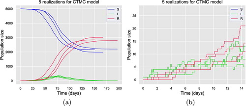
Figure 5 represents 5 realizations generated by SSA for the CTMC model (24(24) $\begin{array}{rl}P((S_{1,t+\mathrm{\Delta }t},I_{1,t+\mathrm{\Delta }})-(S_{1,t},I_{1,t})& =(-1,1))=S_{1,t}{\beta }_1[p_1{\displaystyle \frac{I_{1,t}}{N_1}}+p_2{\displaystyle \frac{I_{2,t}}{N_2}}]+o(\mathrm{\Delta }),\\ P((I_{1,t+\mathrm{\Delta }t},R_{1,t+\mathrm{\Delta }})-(I_{1,t},R_{1,t})& =(-1,1))=\gamma I_{1,t}+o(\delta ),\\ P((S_{2,t+\mathrm{\Delta }t},I_{2,t+\mathrm{\Delta }})-(S_{2,t},I_{2,t})& =(-1,1))=S_{2,t}{\beta }_2[p_1{\displaystyle \frac{I_{1,t}}{N_1}}+p_2{\displaystyle \frac{I_{2,t}}{N_2}}]+o(\mathrm{\Delta }),\\ P((I_{2,t+\mathrm{\Delta }t},R_{2,t+\mathrm{\Delta }})-(I_{2,t},R_{2,t})& =(-1,1))=\gamma I_{2,t}+o(\mathrm{\Delta })\end{array}$(24) ) with heterogeneous mixing. The top two subfigures are with initial condition of 1 infectious superspreader and the bottom two subfigures are with initial condition of 1 infectious non-superspreader, respectively. For the top two subfigures, there are 3 realizations representing the major epidemic outbreaks as the numbers of infectious individuals increasing. The other 2 realizations represent the minor outbreaks. For the bottom two subfigures, there is only 1 realization out of 5 representing the successful establishment of the outbreak. Figure 5(a,b) emphasize the early stages of the epidemics for two cases, respectively. The preliminary result of simulations in Figure 5 shows that initiations by superspreaders are more likely to cause the outbreaks.

Figure 5. Five realizations generated by SSA for CTMC model (24(24) $\begin{array}{rl}P((S_{1,t+\mathrm{\Delta }t},I_{1,t+\mathrm{\Delta }})-(S_{1,t},I_{1,t})& =(-1,1))=S_{1,t}{\beta }_1[p_1{\displaystyle \frac{I_{1,t}}{N_1}}+p_2{\displaystyle \frac{I_{2,t}}{N_2}}]+o(\mathrm{\Delta }),\\ P((I_{1,t+\mathrm{\Delta }t},R_{1,t+\mathrm{\Delta }})-(I_{1,t},R_{1,t})& =(-1,1))=\gamma I_{1,t}+o(\delta ),\\ P((S_{2,t+\mathrm{\Delta }t},I_{2,t+\mathrm{\Delta }})-(S_{2,t},I_{2,t})& =(-1,1))=S_{2,t}{\beta }_2[p_1{\displaystyle \frac{I_{1,t}}{N_1}}+p_2{\displaystyle \frac{I_{2,t}}{N_2}}]+o(\mathrm{\Delta }),\\ P((I_{2,t+\mathrm{\Delta }t},R_{2,t+\mathrm{\Delta }})-(I_{2,t},R_{2,t})& =(-1,1))=\gamma I_{2,t}+o(\mathrm{\Delta })\end{array}$(24) ) with heterogeneous mixing. The top two subfigures are with initial condition of 1 infectious superspreader. The bottom two subfigures are with initial condition of 1 infectious non-superspreader.

The second set of numerical simulations is to generate ${10}^4$ realizations by SSA for the CTMC model (21(21) $\begin{array}{rl}P((S_{t+\mathrm{\Delta }t},I_{t+\mathrm{\Delta }t},R_{t+\mathrm{\Delta }t})-(S_t,I_t,R_t)& =(-1,1,0))={\displaystyle \frac{\beta S_t{I}_t}{N}}\mathrm{\Delta }t+o(\mathrm{\Delta }t),\\ P((S_{t+\mathrm{\Delta }t},I_{t+\mathrm{\Delta }t},R_{t+\mathrm{\Delta }t})-(S_t,I_t,R_t)& =(0,-1,1))=\gamma I_t\mathrm{\Delta }t+o(\mathrm{\Delta }t),\end{array}$(21) ) with homogeneous mixing and the CTMC model (24(24) $\begin{array}{rl}P((S_{1,t+\mathrm{\Delta }t},I_{1,t+\mathrm{\Delta }})-(S_{1,t},I_{1,t})& =(-1,1))=S_{1,t}{\beta }_1[p_1{\displaystyle \frac{I_{1,t}}{N_1}}+p_2{\displaystyle \frac{I_{2,t}}{N_2}}]+o(\mathrm{\Delta }),\\ P((I_{1,t+\mathrm{\Delta }t},R_{1,t+\mathrm{\Delta }})-(I_{1,t},R_{1,t})& =(-1,1))=\gamma I_{1,t}+o(\delta ),\\ P((S_{2,t+\mathrm{\Delta }t},I_{2,t+\mathrm{\Delta }})-(S_{2,t},I_{2,t})& =(-1,1))=S_{2,t}{\beta }_2[p_1{\displaystyle \frac{I_{1,t}}{N_1}}+p_2{\displaystyle \frac{I_{2,t}}{N_2}}]+o(\mathrm{\Delta }),\\ P((I_{2,t+\mathrm{\Delta }t},R_{2,t+\mathrm{\Delta }})-(I_{2,t},R_{2,t})& =(-1,1))=\gamma I_{2,t}+o(\mathrm{\Delta })\end{array}$(24) ) with two different initial conditions. We then estimate the probabilities of a minor outbreak by statistically summarizing the final epidemic sizes of all realizations. The final sizes are defined as $S(\mathrm{initialtime})-S(\mathrm{finaltime})$ for model (21(21) $\begin{array}{rl}P((S_{t+\mathrm{\Delta }t},I_{t+\mathrm{\Delta }t},R_{t+\mathrm{\Delta }t})-(S_t,I_t,R_t)& =(-1,1,0))={\displaystyle \frac{\beta S_t{I}_t}{N}}\mathrm{\Delta }t+o(\mathrm{\Delta }t),\\ P((S_{t+\mathrm{\Delta }t},I_{t+\mathrm{\Delta }t},R_{t+\mathrm{\Delta }t})-(S_t,I_t,R_t)& =(0,-1,1))=\gamma I_t\mathrm{\Delta }t+o(\mathrm{\Delta }t),\end{array}$(21) ) and $S_1(\mathrm{initialtime})+S_2(\mathrm{initialtime})-S_1(\mathrm{finaltime})-S_2(\mathrm{finaltime})$ for model (24(24) $\begin{array}{rl}P((S_{1,t+\mathrm{\Delta }t},I_{1,t+\mathrm{\Delta }})-(S_{1,t},I_{1,t})& =(-1,1))=S_{1,t}{\beta }_1[p_1{\displaystyle \frac{I_{1,t}}{N_1}}+p_2{\displaystyle \frac{I_{2,t}}{N_2}}]+o(\mathrm{\Delta }),\\ P((I_{1,t+\mathrm{\Delta }t},R_{1,t+\mathrm{\Delta }})-(I_{1,t},R_{1,t})& =(-1,1))=\gamma I_{1,t}+o(\delta ),\\ P((S_{2,t+\mathrm{\Delta }t},I_{2,t+\mathrm{\Delta }})-(S_{2,t},I_{2,t})& =(-1,1))=S_{2,t}{\beta }_2[p_1{\displaystyle \frac{I_{1,t}}{N_1}}+p_2{\displaystyle \frac{I_{2,t}}{N_2}}]+o(\mathrm{\Delta }),\\ P((I_{2,t+\mathrm{\Delta }t},R_{2,t+\mathrm{\Delta }})-(I_{2,t},R_{2,t})& =(-1,1))=\gamma I_{2,t}+o(\mathrm{\Delta })\end{array}$(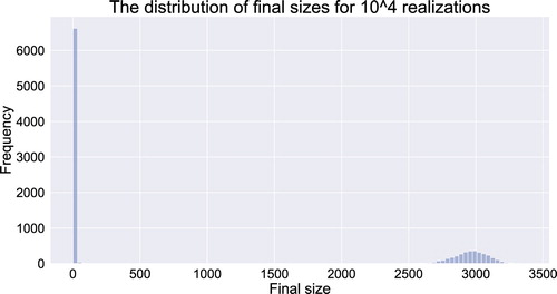24) ), respectively. If the final epidemic size is less than the pre-defined threshold 100, we consider there is a minor outbreak. While if the final epidemic size is larger, we consider there is a major outbreak. Other pre-defined thresholds with relatively small values also work. This is because the distributions of final sizes for stochastic epidemic models are well-known as bimodal (also discussed in [22]), there are very few falling in between.

The result of numerical simulations of ${10}^4$ realizations for CTMC model (21(21) $\begin{array}{rl}P((S_{t+\mathrm{\Delta }t},I_{t+\mathrm{\Delta }t},R_{t+\mathrm{\Delta }t})-(S_t,I_t,R_t)& =(-1,1,0))={\displaystyle \frac{\beta S_t{I}_t}{N}}\mathrm{\Delta }t+o(\mathrm{\Delta }t),\\ P((S_{t+\mathrm{\Delta }t},I_{t+\mathrm{\Delta }t},R_{t+\mathrm{\Delta }t})-(S_t,I_t,R_t)& =(0,-1,1))=\gamma I_t\mathrm{\Delta }t+o(\mathrm{\Delta }t),\end{array}$(21) ) are presented in Figure 6. The distribution of final epidemic sizes indicates that the proportion of realizations with the final size smaller than the pre-defined value 100 is 0.6608. The estimated probability of a minor outbreak by BP is $q_{\star }=\frac{1}{{\mathcal{R}}_0}=\frac{1}{1.5147}=0.6602$.

Figure 6. The distribution of final epidemic sizes for ${10}^4$ realizations for CTMC model (21(21) $\begin{array}{rl}P((S_{t+\mathrm{\Delta }t},I_{t+\mathrm{\Delta }t},R_{t+\mathrm{\Delta }t})-(S_t,I_t,R_t)& =(-1,1,0))={\displaystyle \frac{\beta S_t{I}_t}{N}}\mathrm{\Delta }t+o(\mathrm{\Delta }t),\\ P((S_{t+\mathrm{\Delta }t},I_{t+\mathrm{\Delta }t},R_{t+\mathrm{\Delta }t})-(S_t,I_t,R_t)& =(0,-1,1))=\gamma I_t\mathrm{\Delta }t+o(\mathrm{\Delta }t),\end{array}$(21) ) with homogeneous mixing.

The result of numerical simulations of ${10}^4$ realizations for CTMC model (24(24) $\begin{array}{rl}P((S_{1,t+\mathrm{\Delta }t},I_{1,t+\mathrm{\Delta }})-(S_{1,t},I_{1,t})& =(-1,1))=S_{1,t}{\beta }_1[p_1{\displaystyle \frac{I_{1,t}}{N_1}}+p_2{\displaystyle \frac{I_{2,t}}{N_2}}]+o(\mathrm{\Delta }),\\ P((I_{1,t+\mathrm{\Delta }t},R_{1,t+\mathrm{\Delta }})-(I_{1,t},R_{1,t})& =(-1,1))=\gamma I_{1,t}+o(\delta ),\\ P((S_{2,t+\mathrm{\Delta }t},I_{2,t+\mathrm{\Delta }})-(S_{2,t},I_{2,t})& =(-1,1))=S_{2,t}{\beta }_2[p_1{\displaystyle \frac{I_{1,t}}{N_1}}+p_2{\displaystyle \frac{I_{2,t}}{N_2}}]+o(\mathrm{\Delta }),\\ P((I_{2,t+\mathrm{\Delta }t},R_{2,t+\mathrm{\Delta }})-(I_{2,t},R_{2,t})& =(-1,1))=\gamma I_{2,t}+o(\mathrm{\Delta })\end{array}$(24) ) are presented in Figure 7. The top subfigure is for the case of initiation by 1 infectious superspreader and the bottom subfigure is for the case of initiation by 1 infectious non-superspreader. In Figure 7(a), the proportion of realizations with the final size smaller than the pre-defined value 100 is 0.6591. In Figure 7(b), the proportion of realizations with the final size smaller than the pre-defined value 100 is 0.9699. Thus, we estimate the probabilities of a minor outbreak by performing SSA are $q_1=0.6591$ and $q_2=0.9699$. This conforms the result of $q_1<q_2$ in Theorem 3.2, the initiation by the superspreaders is more likely to cause a major outbreak.

Figure 7. The distributions of final epidemic sizes for ${10}^4$ realizations for CTMC model (24(24) $\begin{array}{rl}P((S_{1,t+\mathrm{\Delta }t},I_{1,t+\mathrm{\Delta }})-(S_{1,t},I_{1,t})& =(-1,1))=S_{1,t}{\beta }_1[p_1{\displaystyle \frac{I_{1,t}}{N_1}}+p_2{\displaystyle \frac{I_{2,t}}{N_2}}]+o(\mathrm{\Delta }),\\ P((I_{1,t+\mathrm{\Delta }t},R_{1,t+\mathrm{\Delta }})-(I_{1,t},R_{1,t})& =(-1,1))=\gamma I_{1,t}+o(\delta ),\\ P((S_{2,t+\mathrm{\Delta }t},I_{2,t+\mathrm{\Delta }})-(S_{2,t},I_{2,t})& =(-1,1))=S_{2,t}{\beta }_2[p_1{\displaystyle \frac{I_{1,t}}{N_1}}+p_2{\displaystyle \frac{I_{2,t}}{N_2}}]+o(\mathrm{\Delta }),\\ P((I_{2,t+\mathrm{\Delta }t},R_{2,t+\mathrm{\Delta }})-(I_{2,t},R_{2,t})& =(-1,1))=\gamma I_{2,t}+o(\mathrm{\Delta })\end{array}$(24) ) with heterogeneous mixing, $(a)$ initiated by 1 infectious superspreader and $(b)$ initiated by 1 infectious non-superspreader.

To verify the second part of Theorem 3.2, we estimate these two probabilities by the formulas in Equations (27(27) $p_2(1-\frac{{\beta }_1}{{\beta }_2})q_2^2+[-\frac{\gamma }{{\beta }_2}+(1+\frac{\gamma }{{\beta }_2})\frac{{\beta }_1}{{\beta }_2}]q_2-\frac{\gamma {\beta }_1}{{\beta }_2^2}=0,$(27) ) and (28(28) $q_1=\frac{q_2}{(1-\frac{{\beta }_1}{{\beta }_2})q_2+\frac{{\beta }_1}{{\beta }_2}}.$(28) ) in the theorem. Based on the parameter values we used for simulations, $q_2$ is determined by the following quadratic equation: (34) $-3q_2^2+144.74q_2-137.32=0.$(34) By solving this equation, we pick the positive root for the estimate of the probability of a minor outbreak by BP, $q_2=0.9683$, which is close to the value we have by SSA. The relation between $q_1$ and $q_2$ in Equation (28(28) $q_1=\frac{q_2}{(1-\frac{{\beta }_1}{{\beta }_2})q_2+\frac{{\beta }_1}{{\beta }_2}}.$(28) ) implies that (35) $q_1=\frac{q_2}{(1-\frac{{\beta }_1}{{\beta }_2})q_2+\frac{{\beta }_1}{{\beta }_2}}=\frac{0.9683}{-0.9683\times 15+16}=\mathrm{0.666.}$(35) Thus, estimates from BP and estimates by SSA show good agreement. We summarize the results of numerical experiments in Table 2.

Table 2. The probability of a minor outbreak for CTMC models (21(21) $\begin{array}{rl}P((S_{t+\mathrm{\Delta }t},I_{t+\mathrm{\Delta }t},R_{t+\mathrm{\Delta }t})-(S_t,I_t,R_t)& =(-1,1,0))={\displaystyle \frac{\beta S_t{I}_t}{N}}\mathrm{\Delta }t+o(\mathrm{\Delta }t),\\ P((S_{t+\mathrm{\Delta }t},I_{t+\mathrm{\Delta }t},R_{t+\mathrm{\Delta }t})-(S_t,I_t,R_t)& =(0,-1,1))=\gamma I_t\mathrm{\Delta }t+o(\mathrm{\Delta }t),\end{array}$(21) ) with initially 1 infectious individual, and (24(24) $\begin{array}{rl}P((S_{1,t+\mathrm{\Delta }t},I_{1,t+\mathrm{\Delta }})-(S_{1,t},I_{1,t})& =(-1,1))=S_{1,t}{\beta }_1[p_1{\displaystyle \frac{I_{1,t}}{N_1}}+p_2{\displaystyle \frac{I_{2,t}}{N_2}}]+o(\mathrm{\Delta }),\\ P((I_{1,t+\mathrm{\Delta }t},R_{1,t+\mathrm{\Delta }})-(I_{1,t},R_{1,t})& =(-1,1))=\gamma I_{1,t}+o(\delta ),\\ P((S_{2,t+\mathrm{\Delta }t},I_{2,t+\mathrm{\Delta }})-(S_{2,t},I_{2,t})& =(-1,1))=S_{2,t}{\beta }_2[p_1{\displaystyle \frac{I_{1,t}}{N_1}}+p_2{\displaystyle \frac{I_{2,t}}{N_2}}]+o(\mathrm{\Delta }),\\ P((I_{2,t+\mathrm{\Delta }t},R_{2,t+\mathrm{\Delta }})-(I_{2,t},R_{2,t})& =(-1,1))=\gamma I_{2,t}+o(\mathrm{\Delta })\end{array}$(24) ) with initially 1 infectious super-spreader and 1 infectious non super-spreader, respectively. It is demonstrated that, even with identical ${\mathcal{R}}_0$, the probability of a minor outbreak can be varied by different choice of epidemic models.

Summary of probabilities of a minor outbreak for CTMC models
Models (initial infection type)	BP estimates	SSA estimates
CTMC model (21(21) $\begin{array}{rl}P((S_{t+\mathrm{\Delta }t},I_{t+\mathrm{\Delta }t},R_{t+\mathrm{\Delta }t})-(S_t,I_t,R_t)& =(-1,1,0))={\displaystyle \frac{\beta S_t{I}_t}{N}}\mathrm{\Delta }t+o(\mathrm{\Delta }t),\\ P((S_{t+\mathrm{\Delta }t},I_{t+\mathrm{\Delta }t},R_{t+\mathrm{\Delta }t})-(S_t,I_t,R_t)& =(0,-1,1))=\gamma I_t\mathrm{\Delta }t+o(\mathrm{\Delta }t),\end{array}$(21) )	0.6602	0.6608
CTMC model (24(24) $\begin{array}{rl}P((S_{1,t+\mathrm{\Delta }t},I_{1,t+\mathrm{\Delta }})-(S_{1,t},I_{1,t})& =(-1,1))=S_{1,t}{\beta }_1[p_1{\displaystyle \frac{I_{1,t}}{N_1}}+p_2{\displaystyle \frac{I_{2,t}}{N_2}}]+o(\mathrm{\Delta }),\\ P((I_{1,t+\mathrm{\Delta }t},R_{1,t+\mathrm{\Delta }})-(I_{1,t},R_{1,t})& =(-1,1))=\gamma I_{1,t}+o(\delta ),\\ P((S_{2,t+\mathrm{\Delta }t},I_{2,t+\mathrm{\Delta }})-(S_{2,t},I_{2,t})& =(-1,1))=S_{2,t}{\beta }_2[p_1{\displaystyle \frac{I_{1,t}}{N_1}}+p_2{\displaystyle \frac{I_{2,t}}{N_2}}]+o(\mathrm{\Delta }),\\ P((I_{2,t+\mathrm{\Delta }t},R_{2,t+\mathrm{\Delta }})-(I_{2,t},R_{2,t})& =(-1,1))=\gamma I_{2,t}+o(\mathrm{\Delta })\end{array}$(24) ) (1 super-spreader)	0.6591	0.6660
CTMC model (24(24) $\begin{array}{rl}P((S_{1,t+\mathrm{\Delta }t},I_{1,t+\mathrm{\Delta }})-(S_{1,t},I_{1,t})& =(-1,1))=S_{1,t}{\beta }_1[p_1{\displaystyle \frac{I_{1,t}}{N_1}}+p_2{\displaystyle \frac{I_{2,t}}{N_2}}]+o(\mathrm{\Delta }),\\ P((I_{1,t+\mathrm{\Delta }t},R_{1,t+\mathrm{\Delta }})-(I_{1,t},R_{1,t})& =(-1,1))=\gamma I_{1,t}+o(\delta ),\\ P((S_{2,t+\mathrm{\Delta }t},I_{2,t+\mathrm{\Delta }})-(S_{2,t},I_{2,t})& =(-1,1))=S_{2,t}{\beta }_2[p_1{\displaystyle \frac{I_{1,t}}{N_1}}+p_2{\displaystyle \frac{I_{2,t}}{N_2}}]+o(\mathrm{\Delta }),\\ P((I_{2,t+\mathrm{\Delta }t},R_{2,t+\mathrm{\Delta }})-(I_{2,t},R_{2,t})& =(-1,1))=\gamma I_{2,t}+o(\mathrm{\Delta })\end{array}$(24) ) (1 non super-spreader)	0.9699	0.9683

Other numerical simulations with other combinations of parameter values are tested, the results on the probabilities of a minor outbreak estimated by BP are confirmed by performing SSA.

4. Conclusion and future work

Given the identical basic reproduction number ${\mathcal{R}}_0$, several deterministic epidemic models and continuous-time Markov chain (CTMC) epidemic models are formulated and studied. In the study of deterministic modelling, we mainly examine the final epidemic sizes predicted by the epidemic models. The relation between the final size and ${\mathcal{R}}_0$ is investigated as well. It has been proved that, by including the behaviour changes and the heterogeneity of activity levels, the predicted final sizes are smaller than the final size for the model with homogeneous mixing. We may conclude that the epidemic models with homogeneous mixing predict the worst scenarios. In CTMC modelling, as the behavioural change does not affect the early phases, two models with homogeneous mixing and heterogeneous mixing are mainly studied. For the CTMC model with homogeneous mixing, the well-known result on the probability of a minor outbreak is simply presented. For the CTMC model with heterogeneous mixing, only the heterogeneity caused by different activity levels is considered. For the CTMC model with two sub-groups, the probability of a minor outbreak which is initiated by superspreaders is smaller than the probability of a minor outbreak which is initiated by non-superspreaders. Both probabilities are calculated explicitly. We also perform several numerical simulation for deterministic modelling and apply stochastic simulation algorithm (SSA) to simulate the CTMC models. All theoretical results are confirmed by the numerical simulations.

It has been suggested in [13] that, in order to measure the behavioural changes in the affected population, it is informative to estimate both the basic reproduction number ${\mathcal{R}}_0$ and the effective reproduction numbers with respect to time. The early identifications of the superspreaders and the qualifications and inferences of different activity levels are able to improve the formulations of models and thus the predictions on the final sizes. Taking more factors into consideration for the formulations of stochastic models can generate different results regarding the early phases. The heterogeneity of mixing makes predictions about the establishment of major outbreaks more difficult.

The study of heterogeneity of mixing in the population and the investigation on the impact of superspreaders on the transmissions of epidemics are worthy of much efforts. In this paper, we simply assumed that the population can be divided into two sub-groups, based on different activity levels. And for each sub-group, the averaged contact rate is assumed. This assumption is overly simple. It is discussed in [25] that the degree of infectiousness may follow one type of continuous distributions in the population. Then if the infectious period is assumed to be exponential distributed, it is more reasonable to assume that the contact rate β is continuously distributed as well. The second direction of modelling superspreading is to assume that the number of superspreaders is extremely small. For this kind of stochastic model, the method of conditional moments (MCM) [23] might be a good way to investigate.

Acknowledgments

The author thanks his Ph.D. supervisor Dr Fred Brauer from the University of British Columbia for discussions on this topic, reading the manuscripts and providing some proofs. The author also thanks two anonymous reviewers and the editor for their valuable comments and suggestions on the original manuscript. The work is funded by the Post-doctoral fellowship offered by Hausdorff Center for Mathematics and the University of Bonn.

Disclosure statement

No potential conflict of interest was reported by the author(s).

Notes

There is one infectious individual initially for all models. For two epidemic models (12(12) $\begin{array}{rl}{S}_1^{\mathrm{\prime }}& =-S_1[p_{11}{\beta }_1{\displaystyle \frac{I_1}{N_1}}+p_{12}{\beta }_1{\displaystyle \frac{I_2}{N_2}}],\\ I_1^{\mathrm{\prime }}& =S_1[p_{11}{\beta }_1{\displaystyle \frac{I_1}{N_1}}+p_{12}{\beta }_1{\displaystyle \frac{I_2}{N_2}}]-\gamma I_1,\\ R_1^{\mathrm{\prime }}& =\gamma I_1,\\ S_2^{\mathrm{\prime }}& =-S_2[p_{21}{\beta }_2{\displaystyle \frac{I_1}{N_1}}+p_{22}{\beta }_2{\displaystyle \frac{I_2}{N_2}}],\\ I_2^{\mathrm{\prime }}& =S_2[p_{21}{\beta }_2{\displaystyle \frac{I_1}{N_1}}+p_{22}{\beta }_2{\displaystyle \frac{I_2}{N_2}}]-\gamma I_2,\\ R_2^{\mathrm{\prime }}& =\gamma I_2.\end{array}$(12) ) and (19(19) $\begin{array}{rl}{S}_1^{\mathrm{\prime }}& =-S_1{a}_1(t)[p_1{\displaystyle \frac{I_1}{N_1}}+p_2{\displaystyle \frac{I_2}{N_2}}],\\ I_1^{\mathrm{\prime }}& =S_1{a}_1(t)[p_1{\displaystyle \frac{I_1}{N_1}}+p_2{\displaystyle \frac{I_2}{N_2}}]-\gamma I_1,\\ R_1^{\mathrm{\prime }}& =\gamma I_1,\\ S_2^{\mathrm{\prime }}& =-S_2{a}_2(t)[p_1{\displaystyle \frac{I_1}{N_1}}+p_2{\displaystyle \frac{I_2}{N_2}}],\\ I_2^{\mathrm{\prime }}& =S_2{a}_2(t)[p_1{\displaystyle \frac{I_1}{N_1}}+p_2{\displaystyle \frac{I_2}{N_2}}]-\gamma I_2,\\ R_2^{\mathrm{\prime }}& =\gamma I_2.\end{array}$(19) ) with heterogeneous mixing, the summation counts the numbers for the group of superspreaders and the group of non-superspreaders, respectively.

References

- L.J.S. Allen, An Introduction to Stochastic Processes with Applications to Biology, 2nd ed., CRC Press, Boca Raton, FL, December 2010.
- L.J.S. Allen, A primer on stochastic epidemic models: Formulation, numerical simulation, and analysis, Infect. Dis. Model. 2(2) (2017), pp. 128–142.
- K.B. Athreya and P.E. Ney, Branching Processes, Springer, Berlin, Heidelberg, 1972.
- F. Bai, Vaccination models in infectious diseases, Ph.D. thesis, University of British Columbia, 2016.
- F. Bai and L.J.S. Allen, Probability of a major infection in a stochastic within-host model with multiple stages, Appl. Math. Lett. 87 (2019), pp. 1–6.
- F. Bai, K.E.S. Huff, and L.J.S. Allen, The effect of delay in viral production in within-host models during early infection, J. Biol. Dyn. 13(sup1) (2018), pp. 47–73.
- N.T.J. Bailey, The Elements of Stochastic Processes with Applications to the Natural Sciences, John Wiley & Sons, New York, 1990.
- F. Ball and D. Clancy, The final size and severity of a generalised stochastic multitype epidemic model, Adv. Appl. Probab. 25(4) (1993), pp. 721–736.
- F. Brauer, The Kermack–McKendrick epidemic model revisited, Math. Biosci. 198(2) (2005), pp. 119–131.
- F. Brauer, Epidemic models with heterogeneous mixing and treatment, Bull. Math. Biol. 70(7) (2008), pp. 1869–1885.
- F. Brauer, Mathematical epidemiology: Past, present, and future, Infect. Dis. Model. 2(2) (2017), pp. 113–127.
- F. Brauer, Early estimates of epidemic final sizes, J. Biol. Dyn. 13 (2018), pp. 23–30.
- F. Brauer, The final size of a serious epidemic, Bull. Math. Biol. 81(3) (2018), pp. 869–877.
- F. Brauer and C. Castillo-Chavez, Mathematical Models in Population Biology and Epidemiology, Springer, New York, 2012.
- F. Brauer, P. van den Driessche, and J. Wu, Mathematical Epidemiology, Springer, Berlin, Heidelberg, 2008.
- T. Britton, Stochastic epidemic models: A survey, Math. Biosci. 225(1) (2010), pp. 24–35.
- G. Chowell, C. Viboud, J.M. Hyman, etal, The Western Africa Ebola virus disease epidemic exhibits both global exponential and local polynomial growth rates, PLoS Curr. 7 (2015).
- G. Chowell, C. Viboud, L. Simonsen, etal, Characterizing the reproduction number of epidemics with early subexponential growth dynamics, J. R. Soc. Interface 13(123) (2016), p. 20160659.
- S.A. Colgate, E.A. Stanley, J.M. Hyman, S.P. Layne, and C. Qualls, Risk behaviour-based model of the cubic growth of acquired immunodeficiency syndrome in the united states, Proc. Natl Acad. Sci. USA 86(12) (1989), pp. 4793–4797.
- P. van den Driessche and J. Watmough, Reproduction numbers and sub-threshold endemic equilibria for compartmental models of disease transmission, Math. Biosci. 180(1–2) (2002), pp. 29–48.
- A.P. Galvani and R.M. May, Dimensions of superspreading, Nature 438(7066) (2005), pp. 293–295.
- P.E. Greenwood and L.F. Gordillo, Stochastic epidemic modeling, in Chowell, G., Hayman, J.M., Bettencourt, L.M.A., Castillo-Chavez, C. Mathematical and Statistical Estimation Approaches in Epidemiology, Springer, Netherlands, 2009, pp. 31–52.
- J. Hasenauer, V. Wolf, A. Kazeroonian, and F.J. Theis, Method of conditional moments (MCM) for the chemical master equation, J. Math. Biol. 69(3) (2013), pp. 687–735.
- V. Isham, Stochastic models for epidemics, in A. C. Davison and Yadolah Dodge and N. Wermuth. Celebrating Statistics, Oxford: Oxford University Press, 2005, pp. 27–54.
- J.O. Lloyd-Smith, S.J. Schreiber, P.E. Kopp, and W.M. Getz, Superspreading and the effect of individual variation on disease emergence, Nature 438(7066) (2005), pp. 355–359.
- Z. Ma, Y. Zhou, J. Wu, Modeling and Dynamics of Infectious Diseases, Co-Published With Higher Education Press, Beijing, 2009.
- T.R. Maarleveld, B.G. Olivier, and F.J. Bruggeman, StochPy: A comprehensive, user-friendly tool for simulating stochastic biological processes, PLoS ONE 8(11) (2013), p. e79345.
- P. Magal, O. Seydi, and G. Webb, Final size of an epidemic for a two-group SIR model, SIAM J. Appl. Math. 76(5) (2016), pp. 2042–2059.
- P. Magal, O. Seydi, and G. Webb, Final size of a multi-group SIR epidemic model: Irreducible and non-irreducible modes of transmission, Math. Biosci. 301 (2018), pp. 59–67.
- A. Nandi and L.J.S. Allen, Stochastic two-group models with transmission dependent on host infectivity or susceptibility, J. Biol. Dyn. 13(sup1) (2018), pp. 201–224.
- C. Viboud, L. Simonsen, and G. Chowell, A generalized-growth model to characterize the early ascending phase of infectious disease outbreaks, Epidemics 15 (2016), pp. 27–37.
- J. Wallinga and M. Lipsitch, How generation intervals shape the relationship between growth rates and reproductive numbers, Proc. R. Soc. B: Biol. Sci. 274(1609) (2006), pp. 599–604.
- P. Whittle, The outcome of a stochastic epidemic – a note on Bailey's paper, Biometrika 42(1/2) (1955), p. 116.