Threshold dynamics of a HCV model with virus to cell transmission in both liver with CTL immune response and the extrahepatic tissue

Abstract

In this paper, a deterministic model characterizing the within-host infection of Hepatitis C virus (HCV) in intrahepatic and extrahepatic tissues is presented. In addition, the model also includes the effect of the cytotoxic T lymphocyte (CTL) immunity described by a linear activation rate by infected cells. Firstly, the non-negativity and boundedness of solutions of the model are established. Secondly, the basic reproduction number $R_{01}$ and immune reproduction number $R_{02}$ are calculated, respectively. Three equilibria, namely, infection-free, CTL immune response-free and infected equilibrium with CTL immune response are discussed in terms of these two thresholds. Thirdly, the stability of these three equilibria is investigated theoretically as well as numerically. The results show that when $R_{01}<1$, the virus will be cleared out eventually and the CTL immune response will also disappear; when $R_{02}<1<R_{01}$, the virus persists within the host, but the CTL immune response disappears eventually; when $R_{02}>1$, both of the virus and the CTL immune response persist within the host. Finally, a brief discussion will be given.

Keywords:

• Virus to cell infection
• intrahepatic compartment
• extrahepatic compartment
• CTL immune response
• global stability

2010 Mathematics Subject Classifications:

• 34C12
• 34D23
• 92D30

1. Introduction

Viral hepatitis affects approximately 500 million people around the world – more than 10 times the number affected by HIV/AIDS [1]. Different viruses can cause various forms of viral hepatitis. It is estimated that about 71 million people or 1% of the global population are chronically infected with hepatitis C according to the World Health Organization(WHO) Global Hepatitis Report in 2017 [21]. Therefore, it is important to understand the dynamics of HCV infection in order to manage control programmes efficiently.

Hepatitis C virus (HCV) infection can lead to two different outcomes [8]: in a small fraction of patients (15% of cases), the infection can be controlled and cleared from the blood; the rest of the patients become chronic. Chronic HCV is the main cause of chronic liver diseases and cirrhosis leading to liver transplantation (LT) or death [2]. Unfortunately, the early results of transplantation for patients with chronic HCV were discouraging. Mortality rate of liver transplant is very high, and reinfection of the liver graft often occurs [20]. This inevitable post-transplant infection may be related to the existence of an auxiliary compartment [11]. The presence of HCV replicative intermediates has been reported in serum [7], oral mucosa [3] and gastric mucosa [5]. Dahari et al. [4] studied viral loads of 30 patients undergoing liver transplantation and observed the existence of a second replication compartment.

Virus clearance after acute HCV infection is associated with strong and polyclonal CD4 T cell responses, as well as sustained CTL responses. Recently, molecular techniques have provided fundamental insights into the molecular mechanisms of the immune system for HCV infection [16, 18]. In 1996, Nowak and Bangham [15] proposed a simple mathematical model to explore the relation between antiviral immune response and virus load. In 2003, Wodarz [22] extended the model in [15] to investigate the role of CTL and antibody response in HCV infection dynamics and pathology. Zhou et al. [24, 25] considered the CTL immune response against HCV infection. However, the mechanism of CTL action in HCV infection is still not fully understood [6, 9].

Mathematical models have become important tools in analysing the spread and control of HCV epidemic. Dahari et al. [4] constructed a few within-host HCV infection models to describe HCV viral dynamics from the beginning of the anhepatic phase until the first viral increase data point. These models included two compartments of infection, but did not describe the asymptotical viral dynamics after transplantation of the liver. Qesmi et al. [17] proposed a mathematical model of ordinary differential equations to describe the dynamics of the HBV/HCV and its interaction with both liver and blood cells based on [4, 13], and found that the system undergoes either a transcritical or a backward bifurcation. Wodarz and Jansen [23] proposed a model containing infected cells, non-acitived antigen presenting cells (APCs), acitived APCs and CTL, and analysed its complex dynamics.

However, there are very few HCV infection models with two compartments. Based on the existence of a second replication compartment for HCV and the role of CTL immune response against HCV infection, in this paper, we propose a new mathematical model containing another compartment of HCV infection. Then by the analysis of golbal dynamics, these theoretical results will reveal the interaction between HCV and CLT immune response more completely.

This paper is organized as follows. In Section 2, we formulate a new HCV infection model with CTL immune response and give a positively invariant set. Section 3 deals with the existence of equilibria for the model and two important parameters thresholds will be defined. In Section 4, the global stability of equilibria is investigated by using the Routh-Hurwitz criterion and Lyapunov functions. Some numerical examples are shown in Section 5. Finally, the epidemiological meanings of the obtained results are discussed, and the basic reproduction numbers of HCV infection and CTL immune response are given in Section 6.

2. Model formulation

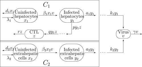
In this section, we formulate a dynamical model with two proliferative compartments of HCV, one of which is the liver, the other is the extrahepatic compartment including serum, peripheral blood mononuclear cells (PBMC), and perihepatic lymph nodes (PLN). No experiments have shown that CTL immune response has effect or no effect on the extrahepatic compartment, here, it is assumed that the CTL immune response takes part in clearing infected hepatocytes and plays no role for the second proliferative compartment. The flowchart of HCV infection is shown in Figure 1. Here, we denote the liver and the second proliferative compartment (extrahepatic compartment) as compartments $C_1$ and $C_2$, respectively. In compartment $C_1$, there are uninfected hepatocytes $(x_1(t)),$ infected hepatocytes $(y_1(t))$ and the CTL immune response $(z(t)).$ In compartment $C_2$, there are uninfected extrahepatic cells $(x_2(t)),$ infected extrahepatic cells $(y_2(t))$ and free virus $(v(t)).$ Following the transmission diagram in Figure 1, our model takes the form in (1(1) $\begin{array}{rl}& x_1^{\prime }={\lambda }_1-{\beta }_1{x}_{1}v-d_1{x}_1,\\ & y_1^{\prime }={\beta }_1{x}_{1}v-a_1{y}_1-p{y}_{1}z,\\ & x_2^{\prime }={\lambda }_2-{\beta }_2{x}_{2}v-d_2{x}_2,\\ & y_2^{\prime }={\beta }_2{x}_{2}v-a_2{y}_2,\\ & v^{\prime }=k_1{y}_1+k_2{y}_2-\gamma v,\\ & z^{\prime }=q{y}_{1}z-rz,\end{array}$(1) ) (1) $\begin{array}{rl}& x_1^{\prime }={\lambda }_1-{\beta }_1{x}_{1}v-d_1{x}_1,\\ & y_1^{\prime }={\beta }_1{x}_{1}v-a_1{y}_1-p{y}_{1}z,\\ & x_2^{\prime }={\lambda }_2-{\beta }_2{x}_{2}v-d_2{x}_2,\\ & y_2^{\prime }={\beta }_2{x}_{2}v-a_2{y}_2,\\ & v^{\prime }=k_1{y}_1+k_2{y}_2-\gamma v,\\ & z^{\prime }=q{y}_{1}z-rz,\end{array}$(1) Here, ${\lambda }_i$ is the recruitment rate of healthy cells and $\frac{1}{d_i}$ is the average lifespan of uninfected cells in compartment $C_i(i=1,2).$ The healthy cells become infected by free virus at a rate ${\beta }_i{x}_{i}v$; infected cells in compartment $C_i(i=1,2)$ die at a rate $a_i{y}_i$, and infected cells in compartment $C_1$ are cleared by the CTL immune response at a rate $p{y}_{1}z$; the CTL immune response is triggered at a rate $q{y}_{1}z$, which in turn decays a rate rz. We assume that the parameters are positive and $a_i\ge d_i(i=1,2)$ [14] according to the biological meaning. Note that a saturated nonlinear function was used in Wodarz and Jansen [23] to describe the activation of the CTL immune response by the virus. Since we are interested in the global dynamics of the model, for the sake of simplicity we use a linear function here.

Figure 1. Flowchart of the viral infection model with CTL immune response in intrahepatic and extrahepatic compartments.

We can see that solutions of model (1(1) $\begin{array}{rl}& x_1^{\prime }={\lambda }_1-{\beta }_1{x}_{1}v-d_1{x}_1,\\ & y_1^{\prime }={\beta }_1{x}_{1}v-a_1{y}_1-p{y}_{1}z,\\ & x_2^{\prime }={\lambda }_2-{\beta }_2{x}_{2}v-d_2{x}_2,\\ & y_2^{\prime }={\beta }_2{x}_{2}v-a_2{y}_2,\\ & v^{\prime }=k_1{y}_1+k_2{y}_2-\gamma v,\\ & z^{\prime }=q{y}_{1}z-rz,\end{array}$(1) ) with the nonnegative initial conditions remain nonnegative. From the first equation of (1(1) $\begin{array}{rl}& x_1^{\prime }={\lambda }_1-{\beta }_1{x}_{1}v-d_1{x}_1,\\ & y_1^{\prime }={\beta }_1{x}_{1}v-a_1{y}_1-p{y}_{1}z,\\ & x_2^{\prime }={\lambda }_2-{\beta }_2{x}_{2}v-d_2{x}_2,\\ & y_2^{\prime }={\beta }_2{x}_{2}v-a_2{y}_2,\\ & v^{\prime }=k_1{y}_1+k_2{y}_2-\gamma v,\\ & z^{\prime }=q{y}_{1}z-rz,\end{array}$(1) ), we have $x_1^{\prime }\le {\lambda }_1-d_1{x}_1,$then $\underset{t\to \mathrm{\infty }}{lim sup}{x}_1(t)\le {\lambda }_1/d_1.$ From the first two equations of (1(1) $\begin{array}{rl}& x_1^{\prime }={\lambda }_1-{\beta }_1{x}_{1}v-d_1{x}_1,\\ & y_1^{\prime }={\beta }_1{x}_{1}v-a_1{y}_1-p{y}_{1}z,\\ & x_2^{\prime }={\lambda }_2-{\beta }_2{x}_{2}v-d_2{x}_2,\\ & y_2^{\prime }={\beta }_2{x}_{2}v-a_2{y}_2,\\ & v^{\prime }=k_1{y}_1+k_2{y}_2-\gamma v,\\ & z^{\prime }=q{y}_{1}z-rz,\end{array}$(1) ), we obtain $(x_1+y_1{)}^{\prime }={\lambda }_1-d_1{x}_1-a_1{y}_1-p{y}_{1}z\le {\lambda }_1-d_1(x_1+y_1),$since $a_1\ge d_1$, then $\underset{t\to \mathrm{\infty }}{lim sup}[x_1(t)+y_1(t)]\le {\lambda }_1/d_1.$ Similarly, from the middle two equations of (1(1) $\begin{array}{rl}& x_1^{\prime }={\lambda }_1-{\beta }_1{x}_{1}v-d_1{x}_1,\\ & y_1^{\prime }={\beta }_1{x}_{1}v-a_1{y}_1-p{y}_{1}z,\\ & x_2^{\prime }={\lambda }_2-{\beta }_2{x}_{2}v-d_2{x}_2,\\ & y_2^{\prime }={\beta }_2{x}_{2}v-a_2{y}_2,\\ & v^{\prime }=k_1{y}_1+k_2{y}_2-\gamma v,\\ & z^{\prime }=q{y}_{1}z-rz,\end{array}$(1) ), we have $\underset{t\to \mathrm{\infty }}{lim sup}{x}_2(t)\le {\lambda }_2/d_2$, and $\underset{t\to \mathrm{\infty }}{lim sup}[x_2(t)+y_2(t)]\le {\lambda }_2/d_2$.

When $y_i\le {\lambda }_i/d_i(i=1,2)$, from the fifth equation of (1(1) $\begin{array}{rl}& x_1^{\prime }={\lambda }_1-{\beta }_1{x}_{1}v-d_1{x}_1,\\ & y_1^{\prime }={\beta }_1{x}_{1}v-a_1{y}_1-p{y}_{1}z,\\ & x_2^{\prime }={\lambda }_2-{\beta }_2{x}_{2}v-d_2{x}_2,\\ & y_2^{\prime }={\beta }_2{x}_{2}v-a_2{y}_2,\\ & v^{\prime }=k_1{y}_1+k_2{y}_2-\gamma v,\\ & z^{\prime }=q{y}_{1}z-rz,\end{array}$(1) ) we have $v^{\prime }\le (\frac{k_1{\lambda }_1}{d_1}+\frac{k_2{\lambda }_2}{d_2})-\gamma v,$then $\underset{t\to \mathrm{\infty }}{lim sup}v(t)\le \frac{1}{\gamma }(\frac{k_1{\lambda }_1}{d_1}+\frac{k_2{\lambda }_2}{d_2}).$And z = 0 always satisfies the last equation in (1(1) $\begin{array}{rl}& x_1^{\prime }={\lambda }_1-{\beta }_1{x}_{1}v-d_1{x}_1,\\ & y_1^{\prime }={\beta }_1{x}_{1}v-a_1{y}_1-p{y}_{1}z,\\ & x_2^{\prime }={\lambda }_2-{\beta }_2{x}_{2}v-d_2{x}_2,\\ & y_2^{\prime }={\beta }_2{x}_{2}v-a_2{y}_2,\\ & v^{\prime }=k_1{y}_1+k_2{y}_2-\gamma v,\\ & z^{\prime }=q{y}_{1}z-rz,\end{array}$(1) ). Therefore, the region $\mathrm{\Omega }=\{(x_1,y_1,x_2,y_2,v,z)\in {\mathbb{R}}_{+}^6:x_i+y_i\le \frac{{\lambda }_i}{d_i},v\le \frac{1}{\gamma }(\frac{k_1{\lambda }_1}{d_1}+\frac{k_2{\lambda }_2}{d_2})(i=1,2)\}$is positively invariant with respect to system (1(1) $\begin{array}{rl}& x_1^{\prime }={\lambda }_1-{\beta }_1{x}_{1}v-d_1{x}_1,\\ & y_1^{\prime }={\beta }_1{x}_{1}v-a_1{y}_1-p{y}_{1}z,\\ & x_2^{\prime }={\lambda }_2-{\beta }_2{x}_{2}v-d_2{x}_2,\\ & y_2^{\prime }={\beta }_2{x}_{2}v-a_2{y}_2,\\ & v^{\prime }=k_1{y}_1+k_2{y}_2-\gamma v,\\ & z^{\prime }=q{y}_{1}z-rz,\end{array}$(1) ). Therefore, it is sufficient to study the dynamics of model (1(1) $\begin{array}{rl}& x_1^{\prime }={\lambda }_1-{\beta }_1{x}_{1}v-d_1{x}_1,\\ & y_1^{\prime }={\beta }_1{x}_{1}v-a_1{y}_1-p{y}_{1}z,\\ & x_2^{\prime }={\lambda }_2-{\beta }_2{x}_{2}v-d_2{x}_2,\\ & y_2^{\prime }={\beta }_2{x}_{2}v-a_2{y}_2,\\ & v^{\prime }=k_1{y}_1+k_2{y}_2-\gamma v,\\ & z^{\prime }=q{y}_{1}z-rz,\end{array}$(1) ) with initial conditions in Ω.

3. Existence of equilibria

In this section, we discuss the existence of equilibria of model (1(1) $\begin{array}{rl}& x_1^{\prime }={\lambda }_1-{\beta }_1{x}_{1}v-d_1{x}_1,\\ & y_1^{\prime }={\beta }_1{x}_{1}v-a_1{y}_1-p{y}_{1}z,\\ & x_2^{\prime }={\lambda }_2-{\beta }_2{x}_{2}v-d_2{x}_2,\\ & y_2^{\prime }={\beta }_2{x}_{2}v-a_2{y}_2,\\ & v^{\prime }=k_1{y}_1+k_2{y}_2-\gamma v,\\ & z^{\prime }=q{y}_{1}z-rz,\end{array}$(1) ) satisfying the following equations (2) $\begin{array}{rl}& {\lambda }_1-{\beta }_1{x}_{1}v-d_1{x}_1=0,\\ & {\beta }_1{x}_{1}v-a_1{y}_1-p{y}_{1}z=0,\\ & {\lambda }_2-{\beta }_2{x}_{2}v-d_2{x}_2=0,\\ & {\beta }_2{x}_{2}v-a_2{y}_2=0,\\ & k_1{y}_1+k_2{y}_2-\gamma v=0,\\ & q{y}_{1}z-rz=0,\end{array}$(2) on the set Ω.

Model (1(1) $\begin{array}{rl}& x_1^{\prime }={\lambda }_1-{\beta }_1{x}_{1}v-d_1{x}_1,\\ & y_1^{\prime }={\beta }_1{x}_{1}v-a_1{y}_1-p{y}_{1}z,\\ & x_2^{\prime }={\lambda }_2-{\beta }_2{x}_{2}v-d_2{x}_2,\\ & y_2^{\prime }={\beta }_2{x}_{2}v-a_2{y}_2,\\ & v^{\prime }=k_1{y}_1+k_2{y}_2-\gamma v,\\ & z^{\prime }=q{y}_{1}z-rz,\end{array}$(1) ) always has an infection-free equilibrium $E_0(x_1^{(0)},0,x_2^{(0)},0,0,0)$, where $x_1^{(0)}=\frac{{\lambda }_1}{d_1},x_2^{(0)}=\frac{{\lambda }_2}{d_2}$. From the first and third equations of (2(2) $\begin{array}{rl}& {\lambda }_1-{\beta }_1{x}_{1}v-d_1{x}_1=0,\\ & {\beta }_1{x}_{1}v-a_1{y}_1-p{y}_{1}z=0,\\ & {\lambda }_2-{\beta }_2{x}_{2}v-d_2{x}_2=0,\\ & {\beta }_2{x}_{2}v-a_2{y}_2=0,\\ & k_1{y}_1+k_2{y}_2-\gamma v=0,\\ & q{y}_{1}z-rz=0,\end{array}$(2) ), we obtain (3) $x_1=\frac{{\lambda }_1}{{\beta }_{1}v+d_1},x_2=\frac{{\lambda }_2}{{\beta }_{2}v+d_2}.$(3) Substituting them into the second and fourth equations of (2(2) $\begin{array}{rl}& {\lambda }_1-{\beta }_1{x}_{1}v-d_1{x}_1=0,\\ & {\beta }_1{x}_{1}v-a_1{y}_1-p{y}_{1}z=0,\\ & {\lambda }_2-{\beta }_2{x}_{2}v-d_2{x}_2=0,\\ & {\beta }_2{x}_{2}v-a_2{y}_2=0,\\ & k_1{y}_1+k_2{y}_2-\gamma v=0,\\ & q{y}_{1}z-rz=0,\end{array}$(2) ), they yields respectively (4) $y_1=\frac{{\beta }_{1}v}{a_1+pz}\cdot \frac{{\lambda }_1}{{\beta }_{1}v+d_1},y_2=\frac{{\beta }_{2}v}{a_2}\cdot \frac{{\lambda }_2}{{\beta }_{2}v+d_2}.$(4) When $v\ne 0$ and z = 0, substituting $y_1$ and $y_2$ of (4(4) $y_1=\frac{{\beta }_{1}v}{a_1+pz}\cdot \frac{{\lambda }_1}{{\beta }_{1}v+d_1},y_2=\frac{{\beta }_{2}v}{a_2}\cdot \frac{{\lambda }_2}{{\beta }_{2}v+d_2}.$(4) ) into the fifth equation of (2(2) $\begin{array}{rl}& {\lambda }_1-{\beta }_1{x}_{1}v-d_1{x}_1=0,\\ & {\beta }_1{x}_{1}v-a_1{y}_1-p{y}_{1}z=0,\\ & {\lambda }_2-{\beta }_2{x}_{2}v-d_2{x}_2=0,\\ & {\beta }_2{x}_{2}v-a_2{y}_2=0,\\ & k_1{y}_1+k_2{y}_2-\gamma v=0,\\ & q{y}_{1}z-rz=0,\end{array}$(2) ) yields (5) $h(v):=\frac{1}{\gamma }[\frac{k_1{\beta }_1{\lambda }_1}{a_1({\beta }_{1}v+d_1)}+\frac{k_2{\beta }_2{\lambda }_2}{a_2({\beta }_{2}v+d_2)}]=1.$(5) We can see that function $h(v)$ is decreasing with respect to v. Note that $h\left(\frac{1}{\gamma }(\frac{k_1{\lambda }_1}{d_1}+\frac{k_2{\lambda }_2}{d_2})\right)\le \frac{1}{1+{\displaystyle \frac{d_1{k}_2{\lambda }_2}{d_2{k}_1{\lambda }_1}}+{\displaystyle \frac{\gamma d_1^2}{k_1{\beta }_1{\lambda }_1}}}+\frac{1}{1+{\displaystyle \frac{d_2{k}_1{\lambda }_1}{d_1{k}_2{\lambda }_2}}+{\displaystyle \frac{\gamma d_2^2}{k_2{\beta }_2{\lambda }_2}}}:=h_0,$where $a_i\ge d_i(i=1,2)$ is used. Since the inequality $\frac{1}{1+m}+\frac{1}{1+n}<1$ holds for m, n>0 if and only if mn>1, we know that $h_0<1$. Thus, by the monotonicity of function $h(v)$, Equation (5(5) $h(v):=\frac{1}{\gamma }[\frac{k_1{\beta }_1{\lambda }_1}{a_1({\beta }_{1}v+d_1)}+\frac{k_2{\beta }_2{\lambda }_2}{a_2({\beta }_{2}v+d_2)}]=1.$(5) ) has a unique positive root $v^{(1)}$ only when $h(0)=\frac{1}{\gamma }[\frac{k_1{\beta }_1{\lambda }_1}{a_1{d}_1}+\frac{k_2{\beta }_2{\lambda }_2}{a_2{d}_2}]>1$. Furthermore, the corresponding $x_i^{(1)}$ and $y_i^{(1)}$ (i = 1, 2) can be obtained from (3(3) $x_1=\frac{{\lambda }_1}{{\beta }_{1}v+d_1},x_2=\frac{{\lambda }_2}{{\beta }_{2}v+d_2}.$(3) ) and (4(4) $y_1=\frac{{\beta }_{1}v}{a_1+pz}\cdot \frac{{\lambda }_1}{{\beta }_{1}v+d_1},y_2=\frac{{\beta }_{2}v}{a_2}\cdot \frac{{\lambda }_2}{{\beta }_{2}v+d_2}.$(4) ). Thus, (1(1) $\begin{array}{rl}& x_1^{\prime }={\lambda }_1-{\beta }_1{x}_{1}v-d_1{x}_1,\\ & y_1^{\prime }={\beta }_1{x}_{1}v-a_1{y}_1-p{y}_{1}z,\\ & x_2^{\prime }={\lambda }_2-{\beta }_2{x}_{2}v-d_2{x}_2,\\ & y_2^{\prime }={\beta }_2{x}_{2}v-a_2{y}_2,\\ & v^{\prime }=k_1{y}_1+k_2{y}_2-\gamma v,\\ & z^{\prime }=q{y}_{1}z-rz,\end{array}$(1) ) has a boundary equilibrium $E_1(x_1^{(1)},y_1^{(1)},x_2^{(1)},$ $y_2^{(1)},v^{(1)},0)$ when $h(0)>1$.

When $z\ne 0$, from the last equation of (2(2) $\begin{array}{rl}& {\lambda }_1-{\beta }_1{x}_{1}v-d_1{x}_1=0,\\ & {\beta }_1{x}_{1}v-a_1{y}_1-p{y}_{1}z=0,\\ & {\lambda }_2-{\beta }_2{x}_{2}v-d_2{x}_2=0,\\ & {\beta }_2{x}_{2}v-a_2{y}_2=0,\\ & k_1{y}_1+k_2{y}_2-\gamma v=0,\\ & q{y}_{1}z-rz=0,\end{array}$(2) ) we have $y_1=\frac{r}{q}:=y_1^{(2)}$. Substituting it and $x_1=\frac{{\lambda }_1}{{\beta }_{1}v+d_1}$ in (3(3) $x_1=\frac{{\lambda }_1}{{\beta }_{1}v+d_1},x_2=\frac{{\lambda }_2}{{\beta }_{2}v+d_2}.$(3) ) into the second equation of (2(2) $\begin{array}{rl}& {\lambda }_1-{\beta }_1{x}_{1}v-d_1{x}_1=0,\\ & {\beta }_1{x}_{1}v-a_1{y}_1-p{y}_{1}z=0,\\ & {\lambda }_2-{\beta }_2{x}_{2}v-d_2{x}_2=0,\\ & {\beta }_2{x}_{2}v-a_2{y}_2=0,\\ & k_1{y}_1+k_2{y}_2-\gamma v=0,\\ & q{y}_{1}z-rz=0,\end{array}$(2) ) gives (6) $z=\frac{q}{pr({\beta }_{1}v+d_1)}[{\beta }_1({\lambda }_1-\frac{a_{1}r}{q})v-\frac{a_1{d}_{1}r}{q}].$(6) Then a necessary condition on the existence of the positive equilibrium is ${\lambda }_1>\frac{a_{1}r}{q}$, and, for the positive equilibrium $E_2(x_1^{(2)},y_1^{(2)},x_2^{(2)},y_2^{(2)},v^{(2)},z^{(2)})$, $v^{(2)}>\frac{a_1{d}_{1}r}{{\beta }_1(q{\lambda }_1-a_{1}r)}:=\overline{v}$.

On the other hand, substituting $y_1=\frac{r}{q}$ and $y_2=\frac{{\beta }_2{\lambda }_{2}v}{a_2({\beta }_{2}v+d_2)}$ in (3(3) $x_1=\frac{{\lambda }_1}{{\beta }_{1}v+d_1},x_2=\frac{{\lambda }_2}{{\beta }_{2}v+d_2}.$(3) ) into the fifth equation of (2(2) $\begin{array}{rl}& {\lambda }_1-{\beta }_1{x}_{1}v-d_1{x}_1=0,\\ & {\beta }_1{x}_{1}v-a_1{y}_1-p{y}_{1}z=0,\\ & {\lambda }_2-{\beta }_2{x}_{2}v-d_2{x}_2=0,\\ & {\beta }_2{x}_{2}v-a_2{y}_2=0,\\ & k_1{y}_1+k_2{y}_2-\gamma v=0,\\ & q{y}_{1}z-rz=0,\end{array}$(2) ) yields (7) $g(v):=\frac{1}{\gamma }[\frac{k_{1}r}{qv}+\frac{k_2{\beta }_2{\lambda }_2}{a_2({\beta }_{2}v+d_2)}]=1.$(7) Under the case that ${\lambda }_1>\frac{a_{1}r}{q}$ (i.e. $\frac{r}{q}<\frac{{\lambda }_1}{a_1}$) and for $a_i\ge d_i$ (i = 1, 2), we have $\begin{array}{rl}g\left(\frac{1}{\gamma }(\frac{k_1{\lambda }_1}{d_1}+\frac{k_2{\lambda }_2}{d_2})\right)& =\frac{r}{q}\cdot \frac{k_1}{{\displaystyle \frac{k_1{\lambda }_1}{d_1}}+{\displaystyle \frac{k_2{\lambda }_2}{d_2}}}+\frac{k_2{\beta }_2{\lambda }_2}{a_2[{\beta }_2({\displaystyle \frac{k_1{\lambda }_1}{d_1}}+\frac{k_2{\lambda }_2}{d_2})+\gamma d_2]}\\ & \le \frac{k_1{\lambda }_1}{a_1({\displaystyle \frac{k_1{\lambda }_1}{d_1}}+{\displaystyle \frac{k_2{\lambda }_2}{d_2}})}+\frac{k_2{\beta }_2{\lambda }_2}{a_2[{\beta }_2({\displaystyle \frac{k_1{\lambda }_1}{d_1}}+{\displaystyle \frac{k_2{\lambda }_2}{d_2}})+\gamma d_2]}\\ & \le \frac{1}{1+{\displaystyle \frac{d_1{k}_2{\lambda }_2}{d_2{k}_1{\lambda }_1}}}+\frac{1}{{\displaystyle \frac{d_2{k}_1{\lambda }_1}{d_1{k}_2{\lambda }_2}}+1+{\displaystyle \frac{\gamma d_2^2}{k_2{\beta }_2{\lambda }_2}}}.\end{array}$Applying again the inequality that $\frac{1}{1+m}+\frac{1}{1+n}<1$ holds for m, n>0 if and only if mn>1, we know that $g\left(\frac{1}{\gamma }(\frac{k_1{\lambda }_1}{d_1}+\frac{k_2{\lambda }_2}{d_2})\right)<1$. Then, according to the monotonicity of function $g(v)$, the fact that $\underset{v\to 0^{+}}{lim}g(v)=+\mathrm{\infty }$ implies that equation $g(v)=1$ has a unique root in the interval $(\overline{v},\frac{1}{\gamma }(\frac{k_1{\lambda }_1}{d_1}+\frac{k_2{\lambda }_2}{d_2}))$ if and only if $g(\overline{v})=\frac{1}{\gamma }\{\frac{k_1{\beta }_1({\lambda }_{1}q-a_{1}r)}{a_1{d}_{1}q}+\frac{k_2{\beta }_2{\lambda }_2}{a_2[{\displaystyle \frac{{\beta }_2{a}_1{d}_{1}r}{{\beta }_1({\lambda }_{1}q-a_{1}r)}}+d_2]}\}>1.$Note that $g(\overline{v})<\frac{1}{\gamma }(\frac{k_1{\beta }_1{\lambda }_1}{a_1{d}_1}+\frac{k_2{\beta }_2{\lambda }_2}{a_2{d}_2})$ as ${\lambda }_1>\frac{a_{1}r}{q}$. Then there must exist a boundary equilibrium $E_1(x_1^{(1)},y_1^{(1)},$ $x_2^{(1)},y_2^{(1)},v^{(1)},0)$ if the positive equilibrium $E_2$ exists.

We claim that for ${\lambda }_1>\frac{a_{1}r}{q}$, $g(\overline{v})>1$ is equivalent to the inequality $\frac{q{\beta }_1{\lambda }_1{v}^{(1)}}{r{a}_1({\beta }_1{v}^{(1)}+d_1)}>1,$ i.e. $v^{(1)}>\overline{v}.$ In fact, since $v=v^{(1)}$ is the root of equation $h(v)=1$, then the monotonicity of $h(v)$ implies that $h(\overline{v})>1$ as $v^{(1)}>\overline{v}.$ On the other hand, direct calculation shows that $g(\overline{v})=h(\overline{v})$. Hence, according the existence of the equilibrium $E_1$, model (1(1) $\begin{array}{rl}& x_1^{\prime }={\lambda }_1-{\beta }_1{x}_{1}v-d_1{x}_1,\\ & y_1^{\prime }={\beta }_1{x}_{1}v-a_1{y}_1-p{y}_{1}z,\\ & x_2^{\prime }={\lambda }_2-{\beta }_2{x}_{2}v-d_2{x}_2,\\ & y_2^{\prime }={\beta }_2{x}_{2}v-a_2{y}_2,\\ & v^{\prime }=k_1{y}_1+k_2{y}_2-\gamma v,\\ & z^{\prime }=q{y}_{1}z-rz,\end{array}$(1) ) has a unique positive equilibrium $E_2$ as $\frac{1}{\gamma }(\frac{k_1{\beta }_1{\lambda }_1}{a_1{d}_1}+\frac{k_2{\beta }_2{\lambda }_2}{a_2{d}_2})>1$, ${\lambda }_1>\frac{a_{1}r}{q}$ and $\frac{q{\beta }_1{\lambda }_1{v}^{(1)}}{r{a}_1({\beta }_1{v}^{(1)}+d_1)}>1,$ i.e. $\frac{q{y}_1^{(1)}}{r}>1$.

Notice that, when $\frac{1}{\gamma }(\frac{k_1{\beta }_1{\lambda }_1}{a_1{d}_1}+\frac{k_2{\beta }_2{\lambda }_2}{a_2{d}_2})>1$, $\frac{q{\beta }_1{\lambda }_1{v}^{(1)}}{r{a}_1({\beta }_1{v}^{(1)}+d_1)}>1$ implies that ${\lambda }_1>\frac{a_{1}r}{q}$. Then, summarizing the above discussion, we have the following theorem.

Theorem 3.1

Denote $R_{01}=\frac{1}{\gamma }(\frac{k_1{\beta }_1{\lambda }_1}{a_1{d}_1}+\frac{k_2{\beta }_2{\lambda }_2}{a_2{d}_2}),R_{02}=\frac{q{y}_1^{(1)}}{r}.$The existence of equilibria in system (1(1) $\begin{array}{rl}& x_1^{\prime }={\lambda }_1-{\beta }_1{x}_{1}v-d_1{x}_1,\\ & y_1^{\prime }={\beta }_1{x}_{1}v-a_1{y}_1-p{y}_{1}z,\\ & x_2^{\prime }={\lambda }_2-{\beta }_2{x}_{2}v-d_2{x}_2,\\ & y_2^{\prime }={\beta }_2{x}_{2}v-a_2{y}_2,\\ & v^{\prime }=k_1{y}_1+k_2{y}_2-\gamma v,\\ & z^{\prime }=q{y}_{1}z-rz,\end{array}$(1) ) can be summarized below.

(a)	The infection-free equilibrium $E_0(x_1^{(0)},0,x_2^{(0)},0,0,0)$ on the set Ω, where $x_1^{(0)}=\frac{{\lambda }_1}{d_1}$ and $x_2^{(0)}=\frac{{\lambda }_2}{d_2},$ always exists.
(b)	When $R_{01}>1$, in addition to the infection-free equilibrium $E_0$, system (1(1) $\begin{array}{rl}& x_1^{\prime }={\lambda }_1-{\beta }_1{x}_{1}v-d_1{x}_1,\\ & y_1^{\prime }={\beta }_1{x}_{1}v-a_1{y}_1-p{y}_{1}z,\\ & x_2^{\prime }={\lambda }_2-{\beta }_2{x}_{2}v-d_2{x}_2,\\ & y_2^{\prime }={\beta }_2{x}_{2}v-a_2{y}_2,\\ & v^{\prime }=k_1{y}_1+k_2{y}_2-\gamma v,\\ & z^{\prime }=q{y}_{1}z-rz,\end{array}$(1) ) also has the immune response-free equilibrium $E_1(x_1^{(1)},y_1^{(1)},x_2^{(1)},$ $y_2^{(1)},v^{(1)},0)$, where $\begin{array}{rl}{x}_1^{(1)}& =\frac{{\lambda }_1}{{\beta }_1{v}^{(1)}+d_1},y_1^{(1)}=\frac{{\beta }_1{\lambda }_1{v}^{(1)}}{a_1({\beta }_1{v}^{(1)}+d_1)},\\ x_2^{(1)}& =\frac{{\lambda }_2}{{\beta }_2{v}^{(1)}+d_2},y_2^{(1)}=\frac{{\beta }_2{\lambda }_2{v}^{(1)}}{a_2({\beta }_2{v}^{(1)}+d_2)},\end{array}$and $v^{(1)}$ is the positive root of (5(5) $h(v):=\frac{1}{\gamma }[\frac{k_1{\beta }_1{\lambda }_1}{a_1({\beta }_{1}v+d_1)}+\frac{k_2{\beta }_2{\lambda }_2}{a_2({\beta }_{2}v+d_2)}]=1.$(5) ).
(c)	When $R_{01}>1$ and $R_{02}>1$, system (1(1) $\begin{array}{rl}& x_1^{\prime }={\lambda }_1-{\beta }_1{x}_{1}v-d_1{x}_1,\\ & y_1^{\prime }={\beta }_1{x}_{1}v-a_1{y}_1-p{y}_{1}z,\\ & x_2^{\prime }={\lambda }_2-{\beta }_2{x}_{2}v-d_2{x}_2,\\ & y_2^{\prime }={\beta }_2{x}_{2}v-a_2{y}_2,\\ & v^{\prime }=k_1{y}_1+k_2{y}_2-\gamma v,\\ & z^{\prime }=q{y}_{1}z-rz,\end{array}$(1) ) has a unique positive equilibrium $E_2(x_1^{(2)},y_1^{(2)},x_2^{(2)},y_2^{(2)},$ $v^{(2)},z^{(2)})$, where $\begin{array}{rl}{x}_1^{(2)}& =\frac{{\lambda }_1}{{\beta }_1{v}^{(2)}+d_1},y_1^{(2)}=\frac{r}{q},\\ x_2^{(2)}& =\frac{{\lambda }_2}{{\beta }_2{v}^{(2)}+d_2},y_2^{(2)}=\frac{{\beta }_2{v}^{(2)}}{a_2}\frac{{\lambda }_2}{{\beta }_2{v}^{(2)}+d_2},z^{(2)}=\frac{a_1}{p}(R_{02}-1)\end{array}$and $v^{(2)}$ is the positive root of (7(7) $g(v):=\frac{1}{\gamma }[\frac{k_{1}r}{qv}+\frac{k_2{\beta }_2{\lambda }_2}{a_2({\beta }_{2}v+d_2)}]=1.$(7) ).

4. Stability of equilibria

In this section, we discuss the global stability of equilibria of (1(1) $\begin{array}{rl}& x_1^{\prime }={\lambda }_1-{\beta }_1{x}_{1}v-d_1{x}_1,\\ & y_1^{\prime }={\beta }_1{x}_{1}v-a_1{y}_1-p{y}_{1}z,\\ & x_2^{\prime }={\lambda }_2-{\beta }_2{x}_{2}v-d_2{x}_2,\\ & y_2^{\prime }={\beta }_2{x}_{2}v-a_2{y}_2,\\ & v^{\prime }=k_1{y}_1+k_2{y}_2-\gamma v,\\ & z^{\prime }=q{y}_{1}z-rz,\end{array}$(1) ). We first present two propositions for the infection-free equilibrium $E_0$.

Proposition 4.1

When $R_{01}<1$, the infection-free equilibrium $E_0$ is locally asymptotically stable; when $R_{01}>1$, it is unstable.

Proof.

The Jacobian matrix of system (1(1) $\begin{array}{rl}& x_1^{\prime }={\lambda }_1-{\beta }_1{x}_{1}v-d_1{x}_1,\\ & y_1^{\prime }={\beta }_1{x}_{1}v-a_1{y}_1-p{y}_{1}z,\\ & x_2^{\prime }={\lambda }_2-{\beta }_2{x}_{2}v-d_2{x}_2,\\ & y_2^{\prime }={\beta }_2{x}_{2}v-a_2{y}_2,\\ & v^{\prime }=k_1{y}_1+k_2{y}_2-\gamma v,\\ & z^{\prime }=q{y}_{1}z-rz,\end{array}$(1) ) at $E_0$ is $J(E_0)=\left(\begin{array}{cccccc}-d_1& 0& 0& 0& -{\beta }_1{\displaystyle \frac{{\lambda }_1}{d_1}}& 0\\ 0& -a_1& 0& 0& {\beta }_1{\displaystyle \frac{{\lambda }_1}{d_1}}& 0\\ 0& 0& -d_2& 0& -{\beta }_2{\displaystyle \frac{{\lambda }_2}{d_2}}& 0\\ 0& 0& 0& -a_2& {\beta }_2{\displaystyle \frac{{\lambda }_2}{d_2}}& 0\\ 0& k_1& 0& k_2& -\gamma & 0\\ 0& 0& 0& 0& 0& -r\end{array}\right).$The eigenvalues of $J(E_0)$ are $-d_1$, $-d_2$, $-r$, and the roots of the equation (8) ${\lambda }^3+b_1{\lambda }^2+b_2\lambda +b_3=0,$(8) where $\begin{array}{rl}{b}_1& =a_1+a_2+\gamma >0,\\ b_2& =a_1{a}_2+(a_1+a_2)\gamma -{\displaystyle \frac{{\beta }_1{\lambda }_1{k}_1}{d_1}}-{\displaystyle \frac{{\beta }_2{\lambda }_2{k}_2}{d_2}}\\ & =a_1{a}_2+a_1\gamma (1-\frac{{\beta }_1{\lambda }_1{k}_1}{a_1{d}_1\gamma })+a_2\gamma (1-\frac{{\beta }_2{\lambda }_2{k}_2}{a_1{d}_2\gamma }),\\ b_3& =a_1{a}_2\gamma (1-R_{01}).\end{array}$Since $R_{01}<1$ implies that $\frac{{\beta }_1{\lambda }_1{k}_1}{a_1{d}_1\gamma }<1\text{and}\frac{{\beta }_2{\lambda }_2{k}_2}{a_1{d}_2\gamma }<1,$we have $b_2>0$ and $b_3>0$ when $R_{01}<1$.

Furthermore, we have $\begin{array}{rl}{b}_1{b}_2-b_3& =(a_1+a_2)a_1{a}_2+a_1{a}_2\gamma R_{01}\\ & +(a_1+a_2+\gamma )[a_1\gamma (1-\frac{{\beta }_1{\lambda }_1{k}_1}{\gamma d_1{a}_1})+a_2\gamma (1-\frac{{\beta }_2{\lambda }_2{k}_2}{\gamma d_2{a}_2})]>0\end{array}$as $R_{01}<1$. It follows from the Routh-Hurwitz criterion that all roots of (8(8) ${\lambda }^3+b_1{\lambda }^2+b_2\lambda +b_3=0,$(8) ) have negative real parts if $R_{01}<1$. Thus, the infection-free equilibrium $E_0$ is locally asymptotically stable when $R_{01}<1$. Since $R_{01}>1$ is equivalent to $b_3<0$, we know that $E_0$ is unstable as $R_{01}>1$.

Proposition 4.2

When $R_{01}<1$, $\underset{t\to \mathrm{\infty }}{lim}{y}_1(t)=\underset{t\to \mathrm{\infty }}{lim}{y}_2(t)=\underset{t\to \mathrm{\infty }}{lim}v(t)=\underset{t\to \mathrm{\infty }}{lim}z(t)=0.$

Proof.

Since $R_{01}<1$, we have $\frac{k_1{\beta }_1{\lambda }_1}{a_1{d}_1\gamma }<1$ and $\frac{k_2{\beta }_2{\lambda }_2}{a_2{d}_2\gamma }<1$, that is, $\frac{{\beta }_1{\lambda }_1}{d_1}<\frac{a_1\gamma }{k_1}$ and $\frac{{\beta }_2{\lambda }_2}{d_2}<\frac{a_2\gamma }{k_2}$. Moreover, direct calculation shows that $R_{01}<1$ is equivalent to the following inequality $0<\frac{{\displaystyle \frac{q{\beta }_1{\lambda }_1}{p{d}_1}}}{{\displaystyle \frac{a_2\gamma }{k_2}}-{\displaystyle \frac{{\beta }_2{\lambda }_2}{d_2}}}<{\displaystyle \frac{{\displaystyle \frac{q}{p}}({\displaystyle \frac{a_1\gamma }{k_1}}-{\displaystyle \frac{{\beta }_1{\lambda }_1}{d_1}})}{{\displaystyle \frac{{\beta }_2{\lambda }_2}{d_2}}}}.$So we can choose a positive number $m_1$ satisfying the inequality (9) $\frac{{\displaystyle \frac{q{\beta }_1{\lambda }_1}{p{d}_1}}}{{\displaystyle \frac{a_2\gamma }{k_2}}-{\displaystyle \frac{{\beta }_2{\lambda }_2}{d_2}}}<m_1<{\displaystyle \frac{{\displaystyle \frac{q}{p}}({\displaystyle \frac{a_1\gamma }{k_1}}-{\displaystyle \frac{{\beta }_1{\lambda }_1}{d_1}})}{{\displaystyle \frac{{\beta }_2{\lambda }_2}{d_2}}}},$(9) that is, $\frac{1}{\gamma }(\frac{q{\beta }_1{\lambda }_1}{p{d}_1}+m_1\frac{{\beta }_2{\lambda }_2}{d_2})<m_1\frac{a_2}{k_2}$and $\frac{1}{\gamma }(\frac{q{\beta }_1{\lambda }_1}{p{d}_1}+m_1\frac{{\beta }_2{\lambda }_2}{d_2})<\frac{q{a}_1}{p{k}_1}.$Further, for the given $m_1$, we choose a positive number $m_2$ satisfying the inequality (10) $\frac{1}{\gamma }(\frac{q{\beta }_1{\lambda }_1}{p{d}_1}+m_1\frac{{\beta }_2{\lambda }_2}{d_2})<m_2<min\{m_1\frac{a_2}{k_2},\frac{q{a}_1}{p{k}_1}\}.$(10) When $m_1$ and $m_2$ are given, we define a function $V_1=\frac{q}{p}{y}_1+m_1{y}_2+m_{2}v+z.$Then $x_1\le \frac{{\lambda }_1}{d_1}$ and $x_2\le \frac{{\lambda }_2}{d_2}$ imply that the derivative of $V_1$ along solutions of model (1(1) $\begin{array}{rl}& x_1^{\prime }={\lambda }_1-{\beta }_1{x}_{1}v-d_1{x}_1,\\ & y_1^{\prime }={\beta }_1{x}_{1}v-a_1{y}_1-p{y}_{1}z,\\ & x_2^{\prime }={\lambda }_2-{\beta }_2{x}_{2}v-d_2{x}_2,\\ & y_2^{\prime }={\beta }_2{x}_{2}v-a_2{y}_2,\\ & v^{\prime }=k_1{y}_1+k_2{y}_2-\gamma v,\\ & z^{\prime }=q{y}_{1}z-rz,\end{array}$(1) ) is given by $\begin{array}{rl}{V}_1^{\prime }& =(m_2{k}_1-\frac{q}{p}{a}_1)y_1+(m_2{k}_2-m_1{a}_2)y_2+(\frac{q}{p}{\beta }_1{x}_1+m_1{\beta }_2{x}_2-m_2\gamma )v-rz\\ & \le -(\frac{q}{p}{a}_1-m_2{k}_1)y_1-(m_1{a}_2-m_2{k}_2)y_2-(m_2\gamma -\frac{q}{p}{\beta }_1\frac{{\lambda }_1}{d_1}-m_1{\beta }_2\frac{{\lambda }_2}{d_2})v-rz.\end{array}$It follows from (9(9) $\frac{{\displaystyle \frac{q{\beta }_1{\lambda }_1}{p{d}_1}}}{{\displaystyle \frac{a_2\gamma }{k_2}}-{\displaystyle \frac{{\beta }_2{\lambda }_2}{d_2}}}<m_1<{\displaystyle \frac{{\displaystyle \frac{q}{p}}({\displaystyle \frac{a_1\gamma }{k_1}}-{\displaystyle \frac{{\beta }_1{\lambda }_1}{d_1}})}{{\displaystyle \frac{{\beta }_2{\lambda }_2}{d_2}}}},$(9) ) and (10(10) $\frac{1}{\gamma }(\frac{q{\beta }_1{\lambda }_1}{p{d}_1}+m_1\frac{{\beta }_2{\lambda }_2}{d_2})<m_2<min\{m_1\frac{a_2}{k_2},\frac{q{a}_1}{p{k}_1}\}.$(10) ) that $\frac{q}{p}{a}_1-m_2{k}_1>0,m_1{a}_2-m_2{k}_2>0,m_2\gamma -\frac{q}{p}{\beta }_1\frac{{\lambda }_1}{d_1}-m_1{\beta }_2\frac{{\lambda }_2}{d_2}>0.$Then $\begin{array}{rl}\rho & =min\{\frac{p}{q}(\frac{q}{p}{a}_1-m_2{k}_1),\frac{1}{m_1}(m_1{a}_2-m_2{k}_2),\frac{1}{m_2}(m_2\gamma -\frac{q}{p}{\beta }_1\frac{{\lambda }_1}{d_1}-m_1{\beta }_2\frac{{\lambda }_2}{d_2}),r\}\\ & >0.\end{array}$Thus, we have $V_1^{\prime }\le -\rho V_1.$ It implies that $\underset{t\to \mathrm{\infty }}{lim}{V}_1(t)=0$, that is, $\underset{t\to \mathrm{\infty }}{lim}{y}_1(t)=\underset{t\to \mathrm{\infty }}{lim}{y}_2(t)=\underset{t\to \mathrm{\infty }}{lim}v(t)=\underset{t\to \mathrm{\infty }}{lim}z(t)=0$.

For the global stability of equilibria of (1(1) $\begin{array}{rl}& x_1^{\prime }={\lambda }_1-{\beta }_1{x}_{1}v-d_1{x}_1,\\ & y_1^{\prime }={\beta }_1{x}_{1}v-a_1{y}_1-p{y}_{1}z,\\ & x_2^{\prime }={\lambda }_2-{\beta }_2{x}_{2}v-d_2{x}_2,\\ & y_2^{\prime }={\beta }_2{x}_{2}v-a_2{y}_2,\\ & v^{\prime }=k_1{y}_1+k_2{y}_2-\gamma v,\\ & z^{\prime }=q{y}_{1}z-rz,\end{array}$(1) ), we have the following results.

Theorem 4.1

When $R_{01}<1,$ the infection-free equilibrium $E_0$ of model (1(1) $\begin{array}{rl}& x_1^{\prime }={\lambda }_1-{\beta }_1{x}_{1}v-d_1{x}_1,\\ & y_1^{\prime }={\beta }_1{x}_{1}v-a_1{y}_1-p{y}_{1}z,\\ & x_2^{\prime }={\lambda }_2-{\beta }_2{x}_{2}v-d_2{x}_2,\\ & y_2^{\prime }={\beta }_2{x}_{2}v-a_2{y}_2,\\ & v^{\prime }=k_1{y}_1+k_2{y}_2-\gamma v,\\ & z^{\prime }=q{y}_{1}z-rz,\end{array}$(1) ) is globally stable in Ω; when $R_{02}<1<R_{01}$, the immune response-free equilibrium $E_1$ of model (1(1) $\begin{array}{rl}& x_1^{\prime }={\lambda }_1-{\beta }_1{x}_{1}v-d_1{x}_1,\\ & y_1^{\prime }={\beta }_1{x}_{1}v-a_1{y}_1-p{y}_{1}z,\\ & x_2^{\prime }={\lambda }_2-{\beta }_2{x}_{2}v-d_2{x}_2,\\ & y_2^{\prime }={\beta }_2{x}_{2}v-a_2{y}_2,\\ & v^{\prime }=k_1{y}_1+k_2{y}_2-\gamma v,\\ & z^{\prime }=q{y}_{1}z-rz,\end{array}$(1) ) is globally stable in $\mathrm{\Omega }\setminus \{E_0\}$; when $R_{01}>1$ and $R_{02}>1$, the infection equilibrium $E_2$ of model (1(1) $\begin{array}{rl}& x_1^{\prime }={\lambda }_1-{\beta }_1{x}_{1}v-d_1{x}_1,\\ & y_1^{\prime }={\beta }_1{x}_{1}v-a_1{y}_1-p{y}_{1}z,\\ & x_2^{\prime }={\lambda }_2-{\beta }_2{x}_{2}v-d_2{x}_2,\\ & y_2^{\prime }={\beta }_2{x}_{2}v-a_2{y}_2,\\ & v^{\prime }=k_1{y}_1+k_2{y}_2-\gamma v,\\ & z^{\prime }=q{y}_{1}z-rz,\end{array}$(1) ) is globally stable in the set Ω.

Proof.

When $R_{01}<1,$ by Proposition 4.2 and the theory of asymptotic autonomous systems [19, Theorem 1.2], it then follows from the first and third equations of (1(1) $\begin{array}{rl}& x_1^{\prime }={\lambda }_1-{\beta }_1{x}_{1}v-d_1{x}_1,\\ & y_1^{\prime }={\beta }_1{x}_{1}v-a_1{y}_1-p{y}_{1}z,\\ & x_2^{\prime }={\lambda }_2-{\beta }_2{x}_{2}v-d_2{x}_2,\\ & y_2^{\prime }={\beta }_2{x}_{2}v-a_2{y}_2,\\ & v^{\prime }=k_1{y}_1+k_2{y}_2-\gamma v,\\ & z^{\prime }=q{y}_{1}z-rz,\end{array}$(1) ) that $x_1(t)\to {\lambda }_1/d_1$ and $x_2(t)\to {\lambda }_2/d_2$ as $t\to +\mathrm{\infty }$. Furthermore, Proposition 4.1 implies that the infection-free equilibrium $E_0$ is globally stable in the set Ω when $R_{01}<1$.

Next, we consider the global stability of the equilibrium $E_1(x_1^{(1)},y_1^{(1)},x_2^{(1)},$ $y_2^{(1)},v^{(1)},0)$. Define a Lyapunov function $\begin{array}{rl}{V}_2& =\frac{k_1}{a_1}(x_1-x_1^{(1)}-x_1^{(1)}\ln \frac{x_1}{x_1^{(1)}}+y_1-y_1^{(1)}-y_1^{(1)}\ln \frac{y_1}{y_1^{(1)}})\\ & +\frac{k_2}{a_2}(x_2-x_2^{(1)}-x_2^{(1)}\ln \frac{x_2}{x_2^{(1)}}+y_2-y_2^{(1)}-y_2^{(1)}\ln \frac{y_2}{y_2^{(1)}})\\ & +(v-v^{(1)}-v^{(1)}\ln \frac{v}{v^{(1)}})+\frac{p{k}_1}{q{a}_1}z,\end{array}$then the derivative of $V_2$ along solutions of system (1(1) $\begin{array}{rl}& x_1^{\prime }={\lambda }_1-{\beta }_1{x}_{1}v-d_1{x}_1,\\ & y_1^{\prime }={\beta }_1{x}_{1}v-a_1{y}_1-p{y}_{1}z,\\ & x_2^{\prime }={\lambda }_2-{\beta }_2{x}_{2}v-d_2{x}_2,\\ & y_2^{\prime }={\beta }_2{x}_{2}v-a_2{y}_2,\\ & v^{\prime }=k_1{y}_1+k_2{y}_2-\gamma v,\\ & z^{\prime }=q{y}_{1}z-rz,\end{array}$(1) ) is given by $\begin{array}{rl}\frac{\mathrm{d}{V}_2}{\mathrm{d}t}& =\frac{k_1}{a_1}[(1-\frac{x_1^{(1)}}{x_1})({\lambda }_1-{\beta }_1{x}_{1}v-d_1{x}_1)+(1-\frac{y_1^{(1)}}{y_1})({\beta }_1{x}_{1}v-a_1{y}_1-p{y}_{1}z)]\\ & +\frac{k_2}{a_2}[(1-\frac{x_2^{(1)}}{x_2})({\lambda }_2-{\beta }_2{x}_{2}v-d_2{x}_2)+(1-\frac{y_2^{(1)}}{y_2})({\beta }_2{x}_{2}v-a_2{y}_2)]\\ & +(1-\frac{v^{(1)}}{v})(k_1{y}_1+k_2{y}_2-\gamma v)+\frac{p{k}_1}{q{a}_1}(q{y}_1-r)z.\end{array}$Since $x_1^{(1)},y_1^{(1)},x_2^{(1)},y_2^{(1)},$ and $v^{(1)}$ satisfy the following equations $\begin{array}{rl}& {\lambda }_1={\beta }_1{x}_{1}v+d_1{x}_1,\\ & {\beta }_1{x}_{1}v=a_1{y}_1,\\ & {\lambda }_2={\beta }_2{x}_{2}v+d_2{x}_2,\\ & {\beta }_2{x}_{2}v=a_2{y}_2,\\ & k_1{y}_1+k_2{y}_2=\gamma v,\end{array}$then $\mathrm{d}{V}_2/\mathrm{d}t$ can be rewritten as follows $\begin{array}{rl}\frac{\mathrm{d}{V}_2}{\mathrm{d}t}& =\frac{k_1{d}_1{x}_1^{(1)}}{a_1}(2-\frac{x_1^{(1)}}{x_1}-\frac{x_1}{x_1^{(1)}})+k_1{y}_1^{(1)}(3-\frac{x_1^{(1)}}{x_1}-\frac{x_{1}v{y}_1^{(1)}}{x_1^{(1)}{v}^{(1)}{y}_1}-\frac{v^{(1)}{y}_1}{v{y}_1^{(1)}})\\ & +\frac{k_2{d}_2{x}_2^{(1)}}{a_2}(2-\frac{x_2^{(1)}}{x_2}-\frac{x_2}{x_2^{(1)}})+k_2{y}_2^{(1)}(3-\frac{x_2^{(1)}}{x_2}-\frac{x_{2}v{y}_2^{(1)}}{x_2^{(1)}{v}^{(1)}{y}_2}-\frac{v^{(1)}{y}_2}{v{y}_2^{(1)}})\\ & +\frac{k_{1}pr}{a_{1}q}(R_{02}-1)z.\end{array}$Since the arithmetical mean is greater than or equal to the geometrical mean, for $x_1,y_1,x_2,y_2,v>0$, we have $\frac{x_1^{(1)}}{x_1}+\frac{x_1}{x_1^{(1)}}-2\ge 0,$ and the equality holds if and only if $x_1=x_1^{(1)}$; $\frac{x_2^{(1)}}{x_2}+\frac{x_2}{x_2^{(1)}}-2\ge 0$, and the equality holds if and only if $x_2=x_2^{(1)}$; $\frac{x_1^{(1)}}{x_1}+\frac{x_{1}v{y}_1^{(1)}}{x_1^{(1)}{v}^{(1)}{y}_1}+\frac{v^{(1)}{y}_1}{v{y}_1^{(1)}}-3\ge 0$, and the equality holds if and only if $x_1=x_1^{(1)}$ and $v/v^{(1)}=y_1/y_1^{(1)}$; $\frac{x_2^{(1)}}{x_2}+\frac{x_{2}v{y}_2^{(1)}}{x_2^{(1)}{v}^{(1)}{y}_2}+\frac{v^{(1)}{y}_2}{v{y}_2^{(1)}}-3\ge 0,$ and the equality holds if and only if $x_2=x_2^{(1)}$ and $v/v^{(1)}=y_2/y_2^{(1)}$.

Therefore, when $R_{02}<1<R_{01}$, we have that $\mathrm{d}{V}_2/\mathrm{d}t\le 0$, and that the equality holds if and only if $x_1=x_1^{(1)}$, $x_2=x_2^{(1)}$, z = 0, and $y_1/y_1^{(1)}=y_2/y_2^{(1)}=v/v^{(1)}$. The largest invariant set of system (1(1) $\begin{array}{rl}& x_1^{\prime }={\lambda }_1-{\beta }_1{x}_{1}v-d_1{x}_1,\\ & y_1^{\prime }={\beta }_1{x}_{1}v-a_1{y}_1-p{y}_{1}z,\\ & x_2^{\prime }={\lambda }_2-{\beta }_2{x}_{2}v-d_2{x}_2,\\ & y_2^{\prime }={\beta }_2{x}_{2}v-a_2{y}_2,\\ & v^{\prime }=k_1{y}_1+k_2{y}_2-\gamma v,\\ & z^{\prime }=q{y}_{1}z-rz,\end{array}$(1) ) on the region $\{(x_1,y_1,x_2,y_2,v,z)\in \mathrm{\Omega }:\mathrm{d}{V}_2/\mathrm{d}t=0\}$ is the singleton $\left\{E_1\right\}$ when $R_{02}<1<R_{01}$. Thus, it follows from LaSalle Invariance Principal [10] that the boundary equilibrium $E_1$ is globally asymptotically stable in the region Ω.

Lastly, we discuss the global stability of the positive equilibrium $E_2(x_1^{(2)},y_1^{(2)},x_2^{(2)},y_2^{(2)},v^{(2)},z^{(2)})$. Define a Lyapunov function $\begin{array}{rl}{V}_3& =\frac{k_1}{a_1+p{z}^{(2)}}(x_1-x_1^{(2)}-x_1^{(2)}\ln \frac{x_1}{x_1^{(2)}}+y_1-y_1^{(2)}-y_1^{(2)}\ln \frac{y_1}{y_1^{(2)}})\\ & +\frac{k_2}{a_2}(x_2-x_2^{(2)}-x_2^{(2)}\ln \frac{x_2}{x_2^{(2)}}+y_2-y_2^{(2)}-y_2^{(2)}\ln \frac{y_2}{y_2^{(2)}})\\ & +(v-v^{(2)}-v^{(2)}\ln \frac{v}{v^{(2)}})+\frac{p{k}_1}{q(a_1+p{z}^{(2)})}(z-z^{(2)}-z^{(2)}\ln \frac{z}{z^{(2)}}),\end{array}$then the derivative of $V_3$ along solutions of system (1(1) $\begin{array}{rl}& x_1^{\prime }={\lambda }_1-{\beta }_1{x}_{1}v-d_1{x}_1,\\ & y_1^{\prime }={\beta }_1{x}_{1}v-a_1{y}_1-p{y}_{1}z,\\ & x_2^{\prime }={\lambda }_2-{\beta }_2{x}_{2}v-d_2{x}_2,\\ & y_2^{\prime }={\beta }_2{x}_{2}v-a_2{y}_2,\\ & v^{\prime }=k_1{y}_1+k_2{y}_2-\gamma v,\\ & z^{\prime }=q{y}_{1}z-rz,\end{array}$(1) ) is given by $\begin{array}{rl}\frac{\mathrm{d}{V}_3}{\mathrm{d}t}& =\frac{k_1}{a_1+p{z}^{(2)}}\\ & \times [(1-\frac{x_1^{(2)}}{x_1})({\lambda }_1-{\beta }_1{x}_{1}v-d_1{x}_1)+(1-\frac{y_1^{(2)}}{y_1})({\beta }_1{x}_{1}v-a_1{y}_1-p{y}_{1}z)]\\ & +\frac{k_2}{a_2}[(1-\frac{x_2^{(1)}}{x_2})({\lambda }_2-{\beta }_2{x}_{2}v-d_2{x}_2)+(1-\frac{y_2^{(2)}}{y_2})({\beta }_2{x}_{2}v-a_2{y}_2)]\\ & +(1-\frac{v^{(2)}}{v})(k_1{y}_1+k_2{y}_2-\gamma v)+\frac{p{k}_1}{q(a_1+p{z}^{(2)})}(1-\frac{z^{(2)}}{z})(q{y}_1-r)z.\end{array}$Using the equalities ${\lambda }_1={\beta }_1{x}_1^{(2)}{v}^{(2)}+d_1{x}_1^{(2)}$, ${\beta }_1{x}_1^{(2)}{v}^{(2)}=a_1{y}_1^{(2)}+p{y}_1^{(2)}{z}^{(2)}$, ${\lambda }_2={\beta }_2{x}_2^{(2)}{v}^{(2)}+d_2{x}_2^{(2)}$, ${\beta }_2{x}_2^{(2)}{v}^{(2)}=a_2{y}_2^{(2)}$, $k_1{y}_1^{(2)}+k_2{y}_2^{(2)}=\gamma v^{(2)}$, and $q{y}_1^{(2)}=r$, we can rewrite $\mathrm{d}{V}_3/\mathrm{d}t$ as follows: $\begin{array}{rl}\frac{\mathrm{d}{V}_3}{\mathrm{d}t}& =\frac{k_1{d}_1{x}_1^{(2)}}{a_1+p{z}^{(2)}}(2-\frac{x_1^{(2)}}{x_1}-\frac{x_1}{x_1^{(2)}})+k_1{y}_1^{(2)}(3-\frac{x_1^{(2)}}{x_1}-\frac{x_{1}v{y}_1^{(2)}}{x_1^{(2)}{v}^{(2)}{y}_1}-\frac{v^{(2)}{y}_1}{v{y}_1^{(2)}})\\ & +\frac{k_2{d}_2{x}_2^{(2)}}{a_2}(2-\frac{x_2^{(2)}}{x_2}-\frac{x_2}{x_2^{(2)}})+k_2{y}_2^{(2)}(3-\frac{x_2^{(2)}}{x_2}-\frac{x_{2}v{y}_2^{(2)}}{x_2^{(2)}{v}^{(2)}{y}_2}-\frac{v^{(2)}{y}_2}{v{y}_2^{(2)}}).\end{array}$Similar to the proof of the global stability of the equilibrium $E_1$, we have that $\mathrm{d}{V}_3/\mathrm{d}t\le 0$, and that the equality holds if and only if $x_1=x_1^{(2)}$, $x_2=x_2^{(2)}$, and $y_1/y_1^{(2)}=y_2/y_2^{(2)}=v/v^{(2)}$. In addition, the largest invariant set of system (1(1) $\begin{array}{rl}& x_1^{\prime }={\lambda }_1-{\beta }_1{x}_{1}v-d_1{x}_1,\\ & y_1^{\prime }={\beta }_1{x}_{1}v-a_1{y}_1-p{y}_{1}z,\\ & x_2^{\prime }={\lambda }_2-{\beta }_2{x}_{2}v-d_2{x}_2,\\ & y_2^{\prime }={\beta }_2{x}_{2}v-a_2{y}_2,\\ & v^{\prime }=k_1{y}_1+k_2{y}_2-\gamma v,\\ & z^{\prime }=q{y}_{1}z-rz,\end{array}$(1) ) on the set $\{(x_1,y_1,x_2,y_2,v,z)\in \mathrm{\Omega }:$ $\mathrm{d}{V}_3/\mathrm{d}t=0\}$ is the singleton $\left\{E_2\right\}$ when $R_{02}>1$. By LaSalle Invariance Principal [10], the positive equilibrium $E_2$ is globally asymptotically stable in the region Ω.

5. Numerical simulations

In the previous sections, we have investigated the existence and global stability of the equilibria through some theoretical analysis. In this section, we will carry out some numerical simulations of (1(1) $\begin{array}{rl}& x_1^{\prime }={\lambda }_1-{\beta }_1{x}_{1}v-d_1{x}_1,\\ & y_1^{\prime }={\beta }_1{x}_{1}v-a_1{y}_1-p{y}_{1}z,\\ & x_2^{\prime }={\lambda }_2-{\beta }_2{x}_{2}v-d_2{x}_2,\\ & y_2^{\prime }={\beta }_2{x}_{2}v-a_2{y}_2,\\ & v^{\prime }=k_1{y}_1+k_2{y}_2-\gamma v,\\ & z^{\prime }=q{y}_{1}z-rz,\end{array}$(1) ) with parameter values ${\lambda }_1=1,{\beta }_1=0.08,d_1=0.2,a_1=0.2,p=0.3,{\lambda }_2=0.8,{\beta }_2=0.1,d_2=0.2,a_2=0.2,k_1=1,k_2=1.2,r=0.2$, except for γ and q. Initial values are fixed in Figure 2–4 at $(5.5,4.7,2.2,2.5,2.2,2.8)$, $(5,4,1.6,1.3,1.0,0.5)$, $(3.8,3,1.2,1.2,0.8,1)$ and $(3.5,2.0,1.3,1.8,1.4,1.2)$. We choose the different values of γ and q to represent different dynamic behaviours. These parameter values chosen here are consistent with those in the models [12, 22, 23].

Figure 2. The infection-free equilibrium $E_0$ is globally asymptotically stable, here $\gamma =5$ and q = 0.1. The other parameter values are fixed as ${\lambda }_1=1,{\beta }_1=0.08,d_1=0.2,a_1=0.2,p=0.3,{\lambda }_2=0.8,{\beta }_2=0.1,d_2=0.2,a_2=0.2,k_1=1,k_2=1.2,r=0.2$, and then $R_{01}=0.88<1$.

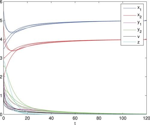
Figure 3. The immune response-free equilibrium $E_1$ is globally asymptotically stable, here $\gamma =2$ and q = 0.06. The other parameter values are identical with those in Figure 2, and then $R_{01}=2.2>1$ and $R_{02}=0.7729<1$.

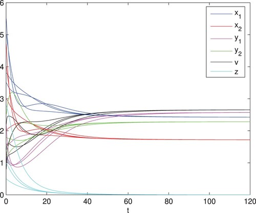
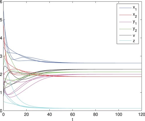
Figure 4. The infection equilibrium $E_2$ is globally asymptotically stable, here $\gamma =2$ and q = 0.1. The other parameter values are identical with those in Figure 2, and then $R_{01}=2.2>1$ and $R_{02}=1.2882>1$.

When $\gamma =5$ and q = 0.1, we calculate $R_{01}=0.88<1$. From Theorem 4.1, it follows that the equilibrium $E_0$ of model (1(1) $\begin{array}{rl}& x_1^{\prime }={\lambda }_1-{\beta }_1{x}_{1}v-d_1{x}_1,\\ & y_1^{\prime }={\beta }_1{x}_{1}v-a_1{y}_1-p{y}_{1}z,\\ & x_2^{\prime }={\lambda }_2-{\beta }_2{x}_{2}v-d_2{x}_2,\\ & y_2^{\prime }={\beta }_2{x}_{2}v-a_2{y}_2,\\ & v^{\prime }=k_1{y}_1+k_2{y}_2-\gamma v,\\ & z^{\prime }=q{y}_{1}z-rz,\end{array}$(1) ) is globally asymptotically stable (see Figure 2). When $\gamma =2$ and q = 0.06, we obtain $R_{01}=2.2>1$ and $R_{02}=0.7729<1.$ From Theorem 4.1, we know that the equilibrium $E_1$ of model (1(1) $\begin{array}{rl}& x_1^{\prime }={\lambda }_1-{\beta }_1{x}_{1}v-d_1{x}_1,\\ & y_1^{\prime }={\beta }_1{x}_{1}v-a_1{y}_1-p{y}_{1}z,\\ & x_2^{\prime }={\lambda }_2-{\beta }_2{x}_{2}v-d_2{x}_2,\\ & y_2^{\prime }={\beta }_2{x}_{2}v-a_2{y}_2,\\ & v^{\prime }=k_1{y}_1+k_2{y}_2-\gamma v,\\ & z^{\prime }=q{y}_{1}z-rz,\end{array}$(1) ) is globally asymptotically stable (see Figure 3). In Figure 4, with parameters $\gamma =2$ and q = 0.1, the thresholds $R_{01}=2.2>1$ and $R_{02}=1.2882>1$. The infection equilibrium $E_2$ of model (1(1) $\begin{array}{rl}& x_1^{\prime }={\lambda }_1-{\beta }_1{x}_{1}v-d_1{x}_1,\\ & y_1^{\prime }={\beta }_1{x}_{1}v-a_1{y}_1-p{y}_{1}z,\\ & x_2^{\prime }={\lambda }_2-{\beta }_2{x}_{2}v-d_2{x}_2,\\ & y_2^{\prime }={\beta }_2{x}_{2}v-a_2{y}_2,\\ & v^{\prime }=k_1{y}_1+k_2{y}_2-\gamma v,\\ & z^{\prime }=q{y}_{1}z-rz,\end{array}$(1) ) is globally asymptotically stable, which is consistent with Theorem 4.1.

6. Conclusion and discussion

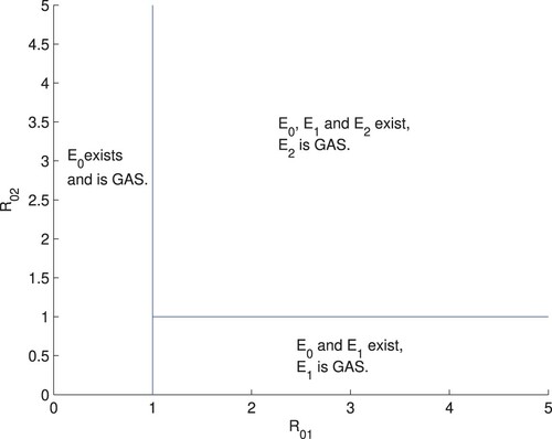
The novelty of our study is that we introduced a new compartment (extrahepatic compartment)) into the classical within-host hepatitis C virus infection models (see Wozard and Jansen [23]) and provided results on the gobal dynamics of the model. According to Theorems 3.1 and 4.1, $R_{01}$ and $R_{02}$ are two thresholds determining the dynamical behaviours of system (1(1) $\begin{array}{rl}& x_1^{\prime }={\lambda }_1-{\beta }_1{x}_{1}v-d_1{x}_1,\\ & y_1^{\prime }={\beta }_1{x}_{1}v-a_1{y}_1-p{y}_{1}z,\\ & x_2^{\prime }={\lambda }_2-{\beta }_2{x}_{2}v-d_2{x}_2,\\ & y_2^{\prime }={\beta }_2{x}_{2}v-a_2{y}_2,\\ & v^{\prime }=k_1{y}_1+k_2{y}_2-\gamma v,\\ & z^{\prime }=q{y}_{1}z-rz,\end{array}$(1) ) (see Figure 5). When $R_{01}<1,$ system (1(1) $\begin{array}{rl}& x_1^{\prime }={\lambda }_1-{\beta }_1{x}_{1}v-d_1{x}_1,\\ & y_1^{\prime }={\beta }_1{x}_{1}v-a_1{y}_1-p{y}_{1}z,\\ & x_2^{\prime }={\lambda }_2-{\beta }_2{x}_{2}v-d_2{x}_2,\\ & y_2^{\prime }={\beta }_2{x}_{2}v-a_2{y}_2,\\ & v^{\prime }=k_1{y}_1+k_2{y}_2-\gamma v,\\ & z^{\prime }=q{y}_{1}z-rz,\end{array}$(1) ) has a unique equilibrium $E_0$, which is globally stable in the set Ω; when $R_{02}<1<R_{01}$, besides the boundary equilibrium $E_0$, system (1(1) $\begin{array}{rl}& x_1^{\prime }={\lambda }_1-{\beta }_1{x}_{1}v-d_1{x}_1,\\ & y_1^{\prime }={\beta }_1{x}_{1}v-a_1{y}_1-p{y}_{1}z,\\ & x_2^{\prime }={\lambda }_2-{\beta }_2{x}_{2}v-d_2{x}_2,\\ & y_2^{\prime }={\beta }_2{x}_{2}v-a_2{y}_2,\\ & v^{\prime }=k_1{y}_1+k_2{y}_2-\gamma v,\\ & z^{\prime }=q{y}_{1}z-rz,\end{array}$(1) ) also has another boundary equilibrium $E_1$, which is globally stable in the set Ω; when $R_{02}>1$, in addition to the boundary equilibria $E_0$ and $E_1$, system (1(1) $\begin{array}{rl}& x_1^{\prime }={\lambda }_1-{\beta }_1{x}_{1}v-d_1{x}_1,\\ & y_1^{\prime }={\beta }_1{x}_{1}v-a_1{y}_1-p{y}_{1}z,\\ & x_2^{\prime }={\lambda }_2-{\beta }_2{x}_{2}v-d_2{x}_2,\\ & y_2^{\prime }={\beta }_2{x}_{2}v-a_2{y}_2,\\ & v^{\prime }=k_1{y}_1+k_2{y}_2-\gamma v,\\ & z^{\prime }=q{y}_{1}z-rz,\end{array}$(1) ) has a unique infection equilibrium $E_2$ which is globally stable in the set Ω.

Figure 5. Existence and stability region of equilibria in terms of the thresholds $R_{01}$ and $R_{02}$.

Notice that $R_{01}=\frac{1}{\gamma }(\frac{k_1{\beta }_1{\lambda }_1}{a_1{d}_1}+\frac{k_2{\beta }_2{\lambda }_2}{a_2{d}_2})$is the basic reproduction number of Hepatitis C virus infection within the host. In fact, $\frac{{\lambda }_1}{d_1}$ is the number of healthy cells at the steady state in compartment $C_1$ in the absence of infection, $\frac{{\beta }_1{\lambda }_1}{d_1}$ is the number of new infected cells in unit time by per capital virion in compartment $C{}_1$, $\frac{k_1}{a_1}$ is the number of new released virion by an infected cell, $\frac{1}{\gamma }$ is the average infectious period of virus, then $\frac{k_1{\beta }_1{\lambda }_1}{a_1{d}_1\gamma }$ is the basic reproduction number of Hepatitis C virus within compartment $C_1$. Similarly, $\frac{k_2{\beta }_2{\lambda }_2}{a_2{d}_2\gamma }$ is the one within compartment $C_2$.

Notice that although $R_{02}$ is the threshold determining the existence and stability of the positive equilibrium $E_2$, it is not the basic reproduction number. From Theorem 3.1, $\frac{q{y}_1^{(1)}}{r}$, denoted by $R_{02}$, can also be thought as a threshold when $R_{01}>1$, which plays the same role as the threshold $R_{02}$ in determining the dynamical behaviours of system (1(1) $\begin{array}{rl}& x_1^{\prime }={\lambda }_1-{\beta }_1{x}_{1}v-d_1{x}_1,\\ & y_1^{\prime }={\beta }_1{x}_{1}v-a_1{y}_1-p{y}_{1}z,\\ & x_2^{\prime }={\lambda }_2-{\beta }_2{x}_{2}v-d_2{x}_2,\\ & y_2^{\prime }={\beta }_2{x}_{2}v-a_2{y}_2,\\ & v^{\prime }=k_1{y}_1+k_2{y}_2-\gamma v,\\ & z^{\prime }=q{y}_{1}z-rz,\end{array}$(1) ). Since $y_1^{(1)}$ is the number of infected cells in compartment $C_1$ at the steady state when $R_{01}>1$, $q{y}_1^{(1)}$ is the CTL immune response existed in a unit time by per CTL response, and $\frac{1}{r}$ is the average decaying period of CTL response, then $\frac{q{y}_1^{(1)}}{r}$ represents the basic reproduction number of the CTL immune response.

For system (1(1) $\begin{array}{rl}& x_1^{\prime }={\lambda }_1-{\beta }_1{x}_{1}v-d_1{x}_1,\\ & y_1^{\prime }={\beta }_1{x}_{1}v-a_1{y}_1-p{y}_{1}z,\\ & x_2^{\prime }={\lambda }_2-{\beta }_2{x}_{2}v-d_2{x}_2,\\ & y_2^{\prime }={\beta }_2{x}_{2}v-a_2{y}_2,\\ & v^{\prime }=k_1{y}_1+k_2{y}_2-\gamma v,\\ & z^{\prime }=q{y}_{1}z-rz,\end{array}$(1) ), we have discussed the existence and stability of three equilibria $E_0$, $E_1$ and $E_2$. In the sense of viral dynamics, the boundary equilibrium $E_0$ represents the infection-free steady state within the host; the other boundary equilibrium $E_1$ represents the steady state at which the host is infected, and the CTL immune response plays no role in protecting the host from infection; the positive equilibrium $E_2$ represents the steady state at which the host is infected and the CTL immune response plays a certain role in protecting the host from infection, but it cannot clear completely the infected cells in compartment $C_1$. Therefore, by Theorems 3.1 and 4.1, when $R_{01}<1$, the virus will be cleared eventually and the CTL immune response also disappears; when $R_{02}<1<R_{01}$, the virus persists within the host, but the CTL immune response disappears eventually, this implies that the immune system in the body of patient has no effect on neutralizing the infection of the virus; when $R_{02}>1$, both the virus and the CTL immune response persist within the host, but the CTL immune response does not suffice to clear the virus completely.

According to the expression of the basic reproduction number of the CTL response $R_{02}$, increasing the coefficient of producing the CTL response q implies the increase of $R_{02}$. Since increasing the value of q results in the decrease of the values of $y_1^{(2)}$, $v^{(2)}$ and $y_2^{(2)}$ for the infetion equilibrium $E_2$, increasing the ability of producing the CTL response can relieve the infetion from viruses.

Disclosure statement

No potential conflict of interest was reported by the author(s).

Additional information

Funding

This work was partially supported by the National Natural Science Foundation of China (No.12061079 and No.11971281),China Postdoctoral Science Foundation [2019M653529], Scientific Research Program funded by Shaanxi Provincial Education Department (No.18JK0336), Cultive Scientific Research Excellence Programs of Higher Education Institutions in Shanxi Provincial Education Department (No.2020KJ020), and Scientific and Technological Innovation Programs of Higher Education Institutions in Shanxi Provincial Education Department (STIP) [2019L0861].

References

- http://www.who.int/bulletin/volumes/88/11/10-011110/en/index.html.
- M.J. Alter, H.S. Margolis, K. Krawczynski, F.N. Judson, A. Mares, W.J. Alexander, P.Y. Hu, J.K. Miller, M.A. Gerber, R.E. Sampliner, E.L. Meeks, and M.J. Beach, The natural history of community-acquired hepatitis C in the United States, N. Engl. J. Med. 327 (1992), pp. 1899–1905.
- M. Carrozzo, R. Quadri, P. Latorre, M. Pentenero, S. Paganin, G. Bertolusso, S. Gandolfo, and F.Negro, Molecular evidence that the hepatitis C virus replicates in the oral mucosa, J. Hepatol. 37 (2002), pp. 364–369.
- H. Dahari, A. Feliu, M. Garcia-Retortillo, X. Forns, and A.U. Neumann, Second hepatitis C replication compartment indicated by viral dynamics during liver transplantation, J. Hepatol. 42 (2005), pp. 491–498.
- S. De Vita, V. De Re, D. Sansonno, D. Sorrentino, R.L. Corte, B. Pivetta, D. Gasparotto, V. Racanelli, A. Marzotto, A. Labombarda, A. Gloghini, G. Ferraccioli, A. Monteverde, A. Carbone, F. Dammacco, and M. Boiocchi, Gastric mucosa as an additional extrahepatic localization of hepatitis C virus: viral detection in gastric low-grade lymphoma associated with autoimmune disease and in chronic gastritis, Hepatology 31 (2000), pp. 182–189.
- P. Farci, A. Shimoda, A. Coiana, G. Diaz, G. Peddis, J.C. Melpolder, A. Strazzera, D.Y. Chien, S.J.Munoz, A. Balestrieri, R.H. Purcell, and H.J. Alter, The outcome of acute hepatitis C predicted by the evolution of the viral quasispecies, Science. 288 (2000), pp. 339–344.
- T.L. Fong, M. Shindo, S.M. Feinstone, J.H. Hoofnagle, and A.M. Di Bisceglie, Detection of replicative intermediates of hepatitis C viral RNA in liver and serum of patients with chronic hepatitis C, J. Clin. Invest. 88 (1991), pp. 1058–1060.
- J.H. Hoofnagle, Management of hepatitis C: current and future perspectives, J. Hepatol 31 (1999), pp. 264–268.
- P. Klenerman, F. Lechner, M. Kantzanou, A. Ciurea, H. Hengartner, and R. Zinkernagel, Viral escape and the failure of cellular immune responses, Science. 289 (2000), p. 2003.
- J.P. LaSalle, The Stability of Dynamical Systems, SIAM, Philadelphia, 1976.
- T. Laskus, M. Radkowski, J. Wilkinson, H. Vargas, and J. Rakela, The origin of hepatitis C virus reinfecting transplanted livers: serum-derived versus peripheral blood mononuclear cell-derived virus, J. Infect. Dis. 185 (2002), pp. 417–421.
- J. Li, K. Men, Y. Yang, and D. Li, Dynamical analysis on a chronic hepattis C virus infection model with immune response, J. Theoret. Biol. 365 (2015), pp. 337–346.
- Y. Liu and X. Liu, Global properties and bifurcation analysis of an HIV-1 infection model with two target cells, Comp. Appl. Math. 37 (2018), pp. 3455–3472.
- A.U. Neumann, N.P. Lam, H. Dahari, D.R. Gretch, T.E. Wiley, T.J. Layden, and A.S. Perelson, Hepatitis C viral dynamics in vivo and the antiviral efficacy of interferon-α therapy, Science. 282 (1998), pp. 103–107.
- M.A. Nowak and C.R.M. Bangham, Population dynamics of immune responses to persistent viruses, Science. 272 (1996), pp. 74–79.
- A. Plauzolles, M. Lucas, and S. Gaudieri, Hepatitis C virus adaptation to T-cell immune pressure, Sci. World J. 2013 (2013), Article ID 673240.
- R. Qesmi, J. Wu, J. Wu, and J.M. Heffernan, Influence of backward bifurcation in a model of hepatitis B and C viruses, Math. Biosci. 224 (2010), pp. 118–125.
- S.D. Sharma, Hepatitis C virus: molecular biology and current therapeutic options, Indian J. Med. Res. 131 (2010), pp. 17–34.
- H.R. Thieme, Convergence results and a Poincaré-Bendison trichotomy for asymptotical autonomous differential equations, J. Math. Biol. 30 (1992), pp. 755–763.
- M. Tsiang, J. Rooney, J. Toole, and C. Gibbs, Biphasic clearance kinetics of hepatitis B virus from patients during adefovir dipivoxil therapy, Hepatology 29 (1999), pp. 1863–1869.
- WHO, Global Hepatitis Report, 2017. France: WHO; 2017.
- D. Wodarz, Hepatitis C virus dynamics and pathology: the role of CTL and antibody responses, J. Gen. Virol. 84 (2003), pp. 1743–1750.
- D. Wodarz and V.A.A. Jansen, A dynamical perspective of CTL cross-priming and regulation: implications for cancer immunology, Immunol. Lett. 86 (2003), pp. 213–227.
- X. Zhou, X. Shi, Z. Zhang, and X. Song, Dynamical behavior of a virus dynamics model with CTL immune response, Appl. Math. Comput. 213 (2009), pp. 329–347.
- Y. Zhou, Y. Zhang, Z. Yao, J.P. Moorman, and Z. Jia, Dendritic cell-based immunity and vaccination agains the patitis C virus infection, Immunology 136 (2012), pp. 385–396.