Transmission rates and environmental reservoirs for COVID-19 – a modeling study

Abstract

The coronavirus disease 2019 (COVID-19) remains a global pandemic at present. Although the human-to-human transmission route for this disease has been well established, its transmission mechanism is not fully understood. In this paper, we propose a mathematical model for COVID-19 which incorporates multiple transmission pathways and which employs time-dependent transmission rates reflecting the impact of disease prevalence and outbreak control. Applying this model to a retrospective study based on publicly reported data in China, we argue that the environmental reservoirs play an important role in the transmission and spread of the coronavirus. This argument is supported by our data fitting and numerical simulation results for the city of Wuhan, for the provinces of Hubei and Guangdong, and for the entire country of China.

Keywords:

• Disease transmission
• compartmental modeling
• data fitting

2010 Mathematics Subject Classification:

• 92D30

1. Introduction

The coronavirus disease 2019 (COVID-19) has led to high morbidity and mortality in China, Europe, and the United States. The disease has spread throughout the world, creating unprecedented challenges in public health. On March 11, 2020, the World Health Organization (WHO) declared COVID-19 as a global pandemic. This pandemic is currently on-going and the number of infections has been fast increasing, with tens of millions of cases reported in over 210 countries and territories.

COVID-19 is caused by a novel coronavirus which is now named severe acute respiratory syndrome coronavirus 2 (SARS-CoV-2). Typical symptoms of the infection include dry cough, fever, fatigue, difficulty in breathing, and bilateral lung infiltration in severe cases [7]. Non-respiratory symptoms such as nausea, vomiting, and diarrhea are also reported in some patients [1,4,27]. SARS-CoV-2 is regarded as the third zoonotic human coronavirus emerging in the current century, after SARS-CoV in 2002 that spread to 37 countries and the Middle East respiratory syndrome coronavirus (MERS-CoV) in 2012 that spread to 27 countries.

In order to better understand the transmission and spread of COVID-19 and to forecast its epidemic development, a number of mathematical and computational models have been proposed (see, e.g. [8,11,13,17,24]). Almost all these models are based on the susceptible-exposed-infected-recovered (SEIR) compartmental framework, exclusively focussed on the direct, human-to-human transmission pathway [1,2]. On the other hand, the role of the environment in the transmission of COVID-19 has been largely neglected in current clinical and theoretical studies and rarely investigated in modeling and simulation [28]. As a result, our knowledge regarding the transmission mechanism and the epidemiological characteristics of COVID-19 remain limited at present [3,15,23,25]

It has been commonly accepted that COVID-19 can be transmitted through direct contact between human hosts, and both the symptomatic and asymptomatic individuals are capable of infecting others [1,14]. In addition, though not well established yet, the indirect transmission pathway from the environment to human hosts is a highly possible route to spread the coronavirus. When infected individuals cough, sneeze or exhale, they release respiratory droplets that contain the coronavirus and most of these droplets would fall on nearby surfaces and objects. Other individuals could catch the virus by touching the contaminated surfaces or objects and then touching their eyes, noses or mouths. Meanwhile, the coronavirus released by infected individuals could float in the air as aerosols and then be breathed in when other people pass by. Such environment-to-human transmission routes, and the success of such a transmission mode, largely rely on the ability of the coronavirus to survive and persist in the environment.

Environmental survival and viability of SARS-CoV were confirmed in [6,27]. A recent study reviewed 22 types of coronaviruses and found that SARS-CoV, MERS-CoV and endemic human coronaviruses can persist on inanimate surfaces such as metal, glass or plastic for up to 9 days [9]. Another experimental study published in March 2020 found that the novel coronavirus (i.e. SARS-CoV-2) was detectable in aerosols for up to 3 hours, on copper for up to 4 hours, on cardboard for up to 24 hours, and on plastic and stainless steel for up to 3 days [22]. These findings that the virus can remain viable and infectious in aerosols for hours and on surfaces for days indicate a high probability and significant risk of environmental transmission, particularly airborne and fomite transmission, for SARS-CoV-2. Additionally, the novel coronavirus has been found in the stool of some infected individuals [4], which may contaminate the aquatic environment through the sewage water and could add another possible route of environmental transmission for COVID-19 [27].

Another limitation in the current modeling studies of COVID-19 is that the transmission rates are typically fixed as constants, rendering simplicity for both mathematical analysis and data fitting. In practice, however, the transmission rates may change with the epidemiological status and may be impacted by the outbreak control. For example, the Chinese government implemented strong disease control measures to fight COVID-19, including large-scale quarantine, intensive tracking of movement and contact, strict isolation of infected individuals, expanded medical facilities, as well as extending the Lunar New Year holiday and demanding the public to stay home. Meanwhile, when the reported infection level is high, people would be motivated to take voluntary action to reduce the contact with the infected individuals and contaminated environment so as to protect themselves and their family members [26]. As a result, the actual transmission rates may decrease even though the outbreak was ascending, leading to a low level of transmission at a time of high disease prevalence. Consequently, reflecting this time and prevalence dependent feature of transmission rates could improve the accuracy in modeling and simulating COVID-19.

In this paper, we aim to characterize the variable transmission rates of COVID-19 and quantify the role of the environmental reservoirs in the transmission of this disease, through a mathematical modeling approach. The environmental reservoirs here, defined in a broad sense, include the air, water, and all surfaces and objects surrounding human individuals. Our model differs from the previously published COVID-19 models by explicitly including both the direct and indirect transmission routes, and by incorporating time-dependent transmission rates that reflect the realistic impact of disease control measures. We apply our model to the retrospective data reported in China, where COVID-19 originally started. We implement data fitting for the city of Wuhan, the provinces of Hubei and Guangdong, as well as the entire country, and conduct numerical simulation and prediction for the epidemic development of COVID-19 in China.

2. Methods

We utilize a mathematical model based on differential equations to investigate the transmission dynamics of COVID-19 in China. The model involves five compartments: the susceptible individuals (denoted by S), the exposed individuals (denoted by E), the infected/infectious individuals (denoted by I), the recovered individuals (denoted by R), and the concentration of the coronavirus in the environment (denoted by V). Both the exposed and infectious individuals are capable of infecting others. Individuals in the exposed class E are in the incubation period and do not show symptoms, whereas individuals in the infectious class I have fully developed disease symptoms and are identified and counted in the publicly reported data. Thus, the E and I compartments in our model contain asymptomatic infected and symptomatic infected individuals, respectively.

The model is described as follows: (1) $\begin{array}{rl}\frac{\mathrm{d}S}{\mathrm{d}t}& =\mathrm{\Lambda }-{\beta }_E(I,t)SE-{\beta }_I(I,t)SI-{\beta }_V(I,t)SV-\mu S,\\ \frac{\mathrm{d}E}{\mathrm{d}t}& ={\beta }_E(I,t)SE+{\beta }_I(I,t)SI+{\beta }_V(I,t)SV-(\alpha +\mu )E,\\ \frac{\mathrm{d}I}{\mathrm{d}t}& =\alpha E-(w+\gamma +\mu )I,\\ \frac{\mathrm{d}R}{\mathrm{d}t}& =\gamma I-\mu R,\\ \frac{\mathrm{d}V}{\mathrm{d}t}& ={\xi }_{1}E+{\xi }_{2}I-\sigma V.\end{array}$(1) The parameter Λ is the population influx rate, μ is the natural death rate for the human hosts, ${\alpha }^{-1}$ is the incubation period, w is the disease induced death rate, γ is the rate of recovery from the infection, ${\xi }_1$ and ${\xi }_2$ are the rates of contributing the coronavirus to the environment by exposed and infectious individuals, respectively, and σ is the removal rate of the coronavirus from the environmental reservoirs. The values of these parameters are discussed in the Appendix, Section A.2.

We incorporate both the human-to-human (i.e. direct) and the environment-to-human (i.e. indirect) transmission routes in this model. The human-to-human transmission occurs between susceptible and exposed individuals, and between susceptible and infectious individuals. We assume a bilinear incidence for each of these transmission pathways. We also assume that each of the transmission rates ${\beta }_E(I,t)$, ${\beta }_I(I,t)$ and ${\beta }_V(I,t)$ depends on the prevalence I and time t; particularly, each one is a non-increasing function of I, given that a higher level of disease prevalence would motivate stronger outbreak control measures that could reduce the transmission rates.

In this study, we consider a time domain of T consecutive days, divided into two time periods: $0\le t\le t^{\ast }$ and $t^{\ast }<t\le T$ for some $t^{\ast }<T$. We employ the following representation for the three transmission rates: (2) $\begin{array}{rl}{\beta }_E(I,t)& =\{\begin{array}{ll}{\beta }_{E0}{\mathrm{e}}^{-cI(t)},& 0\le t\le t^{\ast },\\ {\beta }_{E\ast },& t^{\ast }<t\le T,\end{array}\mathrm{where}{\beta }_{E\ast }={\beta }_{E0}{\mathrm{e}}^{-cI(t^{\ast })};\\ {\beta }_I(I,t)& =\{\begin{array}{ll}{\beta }_{I0}{\mathrm{e}}^{-cI(t)},& 0\le t\le t^{\ast },\\ {\beta }_{I\ast },& t^{\ast }<t\le T,\end{array}\mathrm{where}{\beta }_{I\ast }={\beta }_{I0}{\mathrm{e}}^{-cI(t^{\ast })};\\ {\beta }_V(I,t)& =\{\begin{array}{ll}{\beta }_{V0}{\mathrm{e}}^{-cI(t)},& 0\le t\le t^{\ast },\\ {\beta }_{V\ast },& t^{\ast }<t\le T,\end{array}\mathrm{where}{\beta }_{V\ast }={\beta }_{V0}{\mathrm{e}}^{-cI(t^{\ast })}.\end{array}$(2) In the formulation above, ${\beta }_{E0}$, ${\beta }_{I0}$ and ${\beta }_{V0}$ denote the upper bounds, and c is a positive constant that adjusts the speed of the decay, for these transmission rates when $0\le t\le t^{\ast }$. During this (first) time period, each transmission rate keeps decreasing as the prevalence I increases, due to the implementation of the disease control motivated by the reported infection level. We assume that the impact of the control measures would reach the maximum strength after $t^{\ast }$ days, so that each transmission rate would attain its lower bound and stabilize at that value for $t^{\ast }<t\le T$. Thus, for this (second) time period, each transmission rate becomes a constant, given by ${\beta }_{E\ast }$, ${\beta }_{I\ast }$ and ${\beta }_{V\ast }$, respectively.

Specifically, we set a simulation period of T = 100 days. We start our simulation from January 23, 2020, when the city of Wuhan was placed in quarantine and completely locked down, followed by the nation-wide implementation of a stay-at-home order. We set the length of the first time period as $t^{\ast }=20$ days; i.e. from January 23 to February 11. It is worth mentioning that on February 12, 2020, the national health commission in China started including cases confirmed by clinical diagnosis, which refers to using CT imaging scans to diagnose patients, in addition to those based on the original method of nucleic acid testing kits. Thus, February 12 marks the first day in our second time period (from February 12, 2020 to May 1, 2020), which has a length of 80 days.

Through a sensitivity analysis (see details in the Appendix, Section A.3), we find that the environment-to-human transmission constant ${\beta }_{V0}$, the transmission adjustment parameter c, and the virus shedding rate ${\xi }_1$ are among the most sensitive parameters involved in our model. Meanwhile, the values of these three parameters are not available in the literature as the majority of models published thus far have focussed on the SEIR framework without considering the environmental component of COVID-19, and they have generally applied constant transmission rates which remain fixed in time. Hence, to estimate the values for these three parameters, we fit our model to the daily reported infection data during the first time period, using the standard least squares method. With their estimated values, we then conduct numerical simulation and prediction in the second time period using fixed transmission rates, formulated above.

Hence, our study consists of two major steps: data fitting in the first time period, and simulation and prediction in the second time period. We conduct the data fitting and simulation tasks separately at the city, province and country levels in China. Specifically, we first apply our model to the reported data in Wuhan city, which had been the COVID-19 epicenter until March 2020 when Europe and the US took up this position. We then use the model to study the provinces of Hubei and Guangdong, which have the highest numbers of cases among all provinces in China. Finally we extend our modeling study to the entire country of China.

3. Results

We first conduct the data fitting for Wuhan city from January 23 to February 11, 2020 using our model (1(1) $\begin{array}{rl}\frac{\mathrm{d}S}{\mathrm{d}t}& =\mathrm{\Lambda }-{\beta }_E(I,t)SE-{\beta }_I(I,t)SI-{\beta }_V(I,t)SV-\mu S,\\ \frac{\mathrm{d}E}{\mathrm{d}t}& ={\beta }_E(I,t)SE+{\beta }_I(I,t)SI+{\beta }_V(I,t)SV-(\alpha +\mu )E,\\ \frac{\mathrm{d}I}{\mathrm{d}t}& =\alpha E-(w+\gamma +\mu )I,\\ \frac{\mathrm{d}R}{\mathrm{d}t}& =\gamma I-\mu R,\\ \frac{\mathrm{d}V}{\mathrm{d}t}& ={\xi }_{1}E+{\xi }_{2}I-\sigma V.\end{array}$(1) ) that incorporates both the direct and indirect transmission routes, to estimate the values of the parameters ${\beta }_{V0}$, c and ${\xi }_1$. Based on data reported on January 23, the initial condition for the host population is set as $(S(0),E(0),I(0),R(0))=(8999015,500,475,10)$ [19]. The initial condition for the coronavirus concentration is set as $V(0)=1000$ viruses/ml. Figure 1 shows the numbers of cumulative confirmed cases in Wuhan during this period versus our fitting curve. The parameter values and their $95\mathrm{\%}$ confidence intervals are presented in Table 1. To measure the goodness-of-fit, we calculate the normalized root-mean-square error (NRMSE), which is defined as follows: $\mathrm{NRMSE}=\frac{\sqrt{n\sum _{i=1}^n(y_i-x_i{)}^2}}{\sum _{i=1}^n{x}_i},$where $x_i$ ($1\le i\le n$) are reported data, $y_i$ ($1\le i\le n$) are computed data, and n is the number of data points used. In general, a lower value of NRMSE indicates a better fitting result. We find that the NRMSE for our Wuhan data fitting is 0.0381.

Figure 1. Data fitting result for the cumulative confirmed cases in Wuhan city using both the direct and indirect transmission routes, for a period of 20 days from January 23, 2020 (day 1) to February 11, 2020 (day 20). The circles (in blue) denote the reported cases and the solid line (in red) denotes the fitting result.

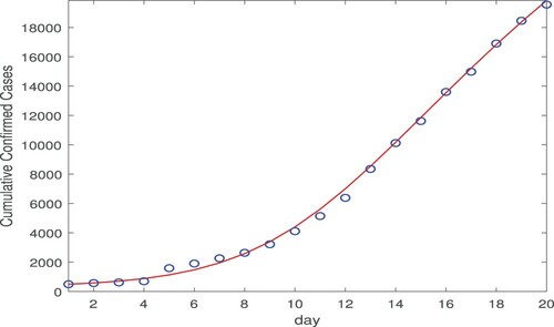
Table 1. Parameter estimates for Wuhan city.

Parameter	Fitting value	95% Confidence interval
${\xi }_1$	33.71	(27.558, 39.856)
${\beta }_{V0}$	$1.10\times {10}^{-9}$	$(0.951\times {10}^{-9},1.245\times {10}^{-9})$
c	$1.65\times {10}^{-4}$	$(1.444\times {10}^{-4},1.857\times {10}^{-4})$

Based on the parameter values from data fitting, we are able to evaluate the basic reproduction number ${\mathcal{R}}_0$ for the disease outbreak in Wuhan during this period; see Equation (A3(A3) $\begin{array}{rl}{\mathcal{R}}_0=\rho (F{V}^{-1})& =\frac{{\beta }_E(0)S_0}{\alpha +\mu }+\frac{\alpha {\beta }_I(0)S_0}{w_1(\alpha +\mu )}+\frac{(w_1{\xi }_1+\alpha {\xi }_2){\beta }_V(0)S_0}{\sigma w_1(\alpha +\mu )},\\ & :={\mathcal{R}}_1+{\mathcal{R}}_2+{\mathcal{R}}_3,\end{array}$(A3) ) in the Appendix for the expression of ${\mathcal{R}}_0$. Estimates of the basic reproduction numbers for COIVD-19 in China range from 2.0 to 7.0 in the literature [3,15]. In our study, we obtain that ${\mathcal{R}}_0=5.11$. In particular, the third component ${\mathcal{R}}_3$ in ${\mathcal{R}}_0$ provides a quantification of the infection risk from the environment-to-human transmission route. We find that ${\mathcal{R}}_3=2.33$, showing a significant contribution from the environmental reservoirs toward the overall infection risk.

As mentioned before, February 12 marks the first day of the second time period in our study where the transmission rates ${\beta }_E(I,t)$, ${\beta }_I(I,t)$ and ${\beta }_V(I,t)$ are fixed as constants, described in Equation (2(2) $\begin{array}{rl}{\beta }_E(I,t)& =\{\begin{array}{ll}{\beta }_{E0}{\mathrm{e}}^{-cI(t)},& 0\le t\le t^{\ast },\\ {\beta }_{E\ast },& t^{\ast }<t\le T,\end{array}\mathrm{where}{\beta }_{E\ast }={\beta }_{E0}{\mathrm{e}}^{-cI(t^{\ast })};\\ {\beta }_I(I,t)& =\{\begin{array}{ll}{\beta }_{I0}{\mathrm{e}}^{-cI(t)},& 0\le t\le t^{\ast },\\ {\beta }_{I\ast },& t^{\ast }<t\le T,\end{array}\mathrm{where}{\beta }_{I\ast }={\beta }_{I0}{\mathrm{e}}^{-cI(t^{\ast })};\\ {\beta }_V(I,t)& =\{\begin{array}{ll}{\beta }_{V0}{\mathrm{e}}^{-cI(t)},& 0\le t\le t^{\ast },\\ {\beta }_{V\ast },& t^{\ast }<t\le T,\end{array}\mathrm{where}{\beta }_{V\ast }={\beta }_{V0}{\mathrm{e}}^{-cI(t^{\ast })}.\end{array}$(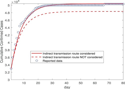2) ). We then conduct numerical simulation using these constant transmission rates for 80 days, from February 12 (day 1) to May 1 (day 80). Figure 2 displays our simulation results for the number of the cumulative cases. Particularly, we compare our simulated curve (shown by the red solid line) against the reported data (shown by the blue circles) from February 12 to May 1, and we observe very good agreement. Indeed, this is confirmed by the NRMSE between the simulated and reported data, which is found as 0.0135. The simulated curve levels off after March 15 (day 33), consistent with the fact that there were almost no new cases reported in Wuhan after March 15 [18,19]. Meanwhile, to illustrate the impact of the environment-to-human transmission pathway on our result, we remove the indirect transmission route from the model and keep only the two direct (exposed-to-susceptible and infectious-to-susceptible) transmission routes, and then repeat the simulation for the same 80-day period. The result, displayed by the red dashed line in Figure 2, clearly shows that the simulated curve deviates from the actual data in this case. Although it is qualitatively evident, the result in Figure 2 provides a quantification on the contribution of the indirect transmission route toward the cumulative number of infections.

Figure 2. Simulation results for the cumulative confirmed cases in Wuhan city based on the data fitting result from Figure 1, for a period of 80 days from February 12, 2020 (day 1) to May 1, 2020 (day 80). The transmission rates are constants in this simulation. The circles (in blue) represent the reported data, and the solid and dashed lines (in red) represent the simulation results with and without incorporating the indirect transmission route, respectively.

To further demonstrate the role of the environment-to-human transmission mode, we conduct both the data fitting in the first time period and the simulation in the second time period using the direct transmission mode only. Specifically, we remove the indirect transmission route from our model (1(1) $\begin{array}{rl}\frac{\mathrm{d}S}{\mathrm{d}t}& =\mathrm{\Lambda }-{\beta }_E(I,t)SE-{\beta }_I(I,t)SI-{\beta }_V(I,t)SV-\mu S,\\ \frac{\mathrm{d}E}{\mathrm{d}t}& ={\beta }_E(I,t)SE+{\beta }_I(I,t)SI+{\beta }_V(I,t)SV-(\alpha +\mu )E,\\ \frac{\mathrm{d}I}{\mathrm{d}t}& =\alpha E-(w+\gamma +\mu )I,\\ \frac{\mathrm{d}R}{\mathrm{d}t}& =\gamma I-\mu R,\\ \frac{\mathrm{d}V}{\mathrm{d}t}& ={\xi }_{1}E+{\xi }_{2}I-\sigma V.\end{array}$(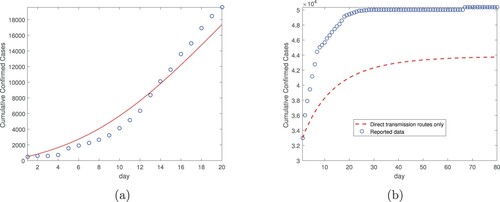1) ) so that only the two direct (exposed-to-susceptible and infectious-to-susceptible) transmission routes are taking effects. Then we conduct the fitting for the same Wuhan data from January 23 to February 11 (20 days), again using the standard least squares method. The result is displayed in Figure 3(a), which shows a clearly larger fitting error compared to that in Figure 1. Based on this fitting result, we then conduction the simulation from February 12 to May 1 (80 days) again using solely the direct transmission routes, and the result is displayed in Figure 3(b). We observe that the simulated curve is significantly below the reported data, a pattern similar to that in Figure 2 (see the dashed line). Together, these fitting and simulation results indicate that we would underestimate the disease burden and the total cumulative cases if the indirect transmission route is not considered.

Figure 3. Data fitting and simulation results for Wuhan city without the indirect transmission route: (a) Data fitting for the cumulative confirmed cases from January 23, 2020 (day 1) to February 11, 2020 (day 20). (b) Simulation for the cumulative confirmed cases based on data fitting from part (a), for a period of 80 days from February 12, 2020 (day 1) to May 1, 2020 (day 80). The transmission rates are constants in the simulation.

Next, we apply the same two-step procedure to Hubei province, which contains Wuhan city. In the data fitting step, we fit our model (1(1) $\begin{array}{rl}\frac{\mathrm{d}S}{\mathrm{d}t}& =\mathrm{\Lambda }-{\beta }_E(I,t)SE-{\beta }_I(I,t)SI-{\beta }_V(I,t)SV-\mu S,\\ \frac{\mathrm{d}E}{\mathrm{d}t}& ={\beta }_E(I,t)SE+{\beta }_I(I,t)SI+{\beta }_V(I,t)SV-(\alpha +\mu )E,\\ \frac{\mathrm{d}I}{\mathrm{d}t}& =\alpha E-(w+\gamma +\mu )I,\\ \frac{\mathrm{d}R}{\mathrm{d}t}& =\gamma I-\mu R,\\ \frac{\mathrm{d}V}{\mathrm{d}t}& ={\xi }_{1}E+{\xi }_{2}I-\sigma V.\end{array}$(1) ) with both the direct and indirect transmission routes to the reported data in Hubei province for 20 days from January 23 to February 11 (i.e. the first time period). The result is presented in Figure 4(a). The values of the three parameters ${\beta }_{V0}$, c and ${\xi }_1$ and their $95\mathrm{\%}$ confidence intervals are presented in Table 2. The NRMSE for this data fitting is 0.0357. The basic reproduction number is ${\mathcal{R}}_0=4.45$, and the component associated with the indirect transmission is ${\mathcal{R}}_3=2.79$. In the simulation step, we fix the three transmission rates ${\beta }_E(I)$, ${\beta }_I(I)$ and ${\beta }_V(I)$ as constants, and conduct numerical simulation for 80 days from February 12 to May 1 (i.e. the second time period). Figure 4(b) shows the simulation results when the indirect transmission route is incorporated and not incorporated, respectively, and the comparison with the reported data from February 12 and May 1. In addition, Figure 4(c,d) display the fitting in period one and simulation in period two, respectively, based on the direct transmission routes only. These results show similar patterns to those in Figures 1–3 and again indicate the significance of the environmental reservoris in transmitting the disease and in shaping the epidemic.

Figure 4. Data fitting and simulation results for Hubei province: (a) Data fitting for the cumulative confirmed cases using both the direct and indirect transmission routes, from January 23, 2020 (day 1) to February 11, 2020 (day 20). The circles denote the reported cases and the solid line denotes the fitting result. (b) Simulation for the cumulative confirmed cases based on data fitting from part (a), for a period of 80 days from February 12, 2020 (day 1) to May 1, 2020 (day 80). The transmission rates are constants in the simulation. (c) Data fitting for the cumulative confirmed cases using the direct transmission routes only, from January 23, 2020 (day 1) to February 11, 2020 (day 20). (d) Simulation for the cumulative confirmed cases based on data fitting from part (c), for a period of 80 days from February 12, 2020 (day 1) to May 1, 2020 (day 80). The transmission rates are constants in the simulation.

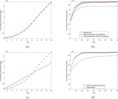
Table 2. Parameter estimates for Hubei province.

Parameter	Fitting value	95% Confidence interval
${\xi }_1$	88.03	(82.211, 93.799)
${\beta }_{V0}$	$7.65\times {10}^{-11}$	$(6.327\times {10}^{-11},8.982\times {10}^{-11})$
c	$9.33\times {10}^{-5}$	$(8.617\times {10}^{-5},10.043\times {10}^{-5})$

We also apply the same fitting-simulation procedure to Guangdong province, which has the second highest number of infections among all provinces in China. The data fitting results with both the direct and indirect routes are presented in Table 3 and Figure 5(a), and the associated simulation results are presented in Figure 5(b). Meanwhile, the fitting and simulation results solely based on the direct transmission routes are displayed in Figure 5(c,d), respectively. Although the infection level in Guangdong province is much lower than that in Hubei province, Figure 5 shows qualitatively similar behaviors, up to March 15, to those in Figure 4. There was a significant increase of the reported cases in Guangdong province after March 15, due to a relatively large number of cases imported from other countries [12], and our model does not account for such imported cases.

Figure 5. Data fitting and simulation results for Guangdong province: (a) Data fitting for the cumulative confirmed cases using both the direct and indirect transmission routes, from January 23, 2020 (day 1) to February 11, 2020 (day 20). (b) Simulation for the cumulative confirmed cases based on data fitting from part (a), for a period of 80 days from February 12, 2020 (day 1) to May 1, 2020 (day 80). (c) Data fitting for the cumulative confirmed cases using the direct transmission routes only, from January 23, 2020 (day 1) to February 11, 2020 (day 20). (d) Simulation for the cumulative confirmed cases based on data fitting from part (c), for a period of 80 days from February 12, 2020 (day 1) to May 1, 2020 (day 80).  The reported cases in Guangdong province increased significantly after March 15 (day 33) due to cases imported from abroad.

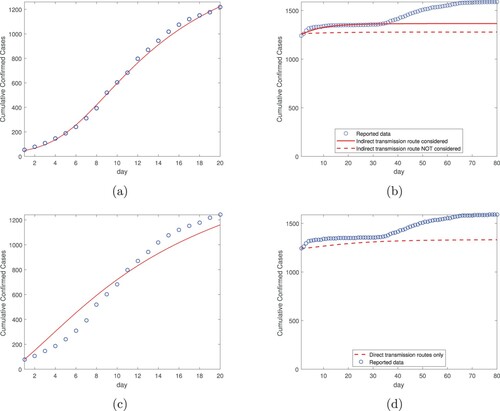
Table 3. Parameter estimates for Guangdong province.

Parameter	Fitting value	95% Confidence interval
${\xi }_1$	79.54	(67.007, 92.068)
${\beta }_{V0}$	$6.94\times {10}^{-11}$	$(2.829\times {10}^{-11},11.043\times {10}^{-11})$
c	$4.55\times {10}^{-3}$	$(4.231\times {10}^{-3},4.867\times {10}^{-3})$

Additionally, we have conducted data fitting and simulation, using the same two-step procedure, for the entire country of China. The results with both the direct and indirect transmission pathways are presented in Table 4 and Figure 6(a,b). The results using only the direct transmission routes are presented in Figure 6(c,d). We observe similar patterns as those at the city and province levels (see Figures 1–5). In particular, based on the data fitting results in the first time period, we observe that the simulation curve in the second time period agrees well with the reported data if incorporating both the direct and indirect transmission routes, and that the numerical prediction would underestimate the infection risk and burden if the indirect transmission route is not included in the model. At the country level, we find the basic reproduction number is ${\mathcal{R}}_0=4.97$, and the indirect transmission associated component is ${\mathcal{R}}_3=2.79$. This again demonstrates the significant role played by the environment-to-human transmission pathway in the spread of COVID-19.

Figure 6. Data fitting and simulation results for the entire country of China: (a) Data fitting for the cumulative confirmed cases using both the direct and indirect transmission routes, from January 23, 2020 (day 1) to February 11, 2020 (day 20). (b) Simulation for the cumulative confirmed cases based on data fitting from part (a), for a period of 80 days from February 12, 2020 (day 1) to May 1, 2020 (day 80). (c) Data fitting for the cumulative confirmed cases using the direct transmission routes only, from January 23, 2020 (day 1) to February 11, 2020 (day 20). (d) Simulation for the cumulative confirmed cases based on data fitting from part (c), for a period of 80 days from February 12, 2020 (day 1) to May 1, 2020 (day 80).

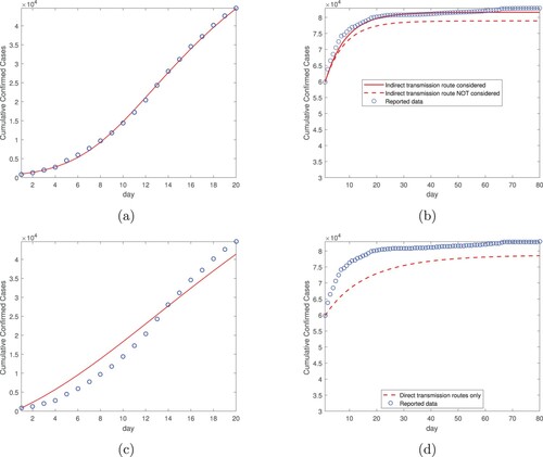
Table 4. Parameter estimates for the entire country of China.

Parameter	Fitting value	95% Confidence interval
${\xi }_1$	42.77	(40.237, 45.298)
${\beta }_{V0}$	$6.23\times {10}^{-12}$	$(2.843\times {10}^{-12},9.612\times {10}^{-12})$
c	$8.53\times {10}^{-5}$	$(8.137\times {10}^{-5},8.928\times {10}^{-5})$

Furthermore, we have conducted a long-term simulation for the disease prevalence $I(t)$ over a period of 200 days starting from February 12, 2020, using our model (1(1) $\begin{array}{rl}\frac{\mathrm{d}S}{\mathrm{d}t}& =\mathrm{\Lambda }-{\beta }_E(I,t)SE-{\beta }_I(I,t)SI-{\beta }_V(I,t)SV-\mu S,\\ \frac{\mathrm{d}E}{\mathrm{d}t}& ={\beta }_E(I,t)SE+{\beta }_I(I,t)SI+{\beta }_V(I,t)SV-(\alpha +\mu )E,\\ \frac{\mathrm{d}I}{\mathrm{d}t}& =\alpha E-(w+\gamma +\mu )I,\\ \frac{\mathrm{d}R}{\mathrm{d}t}& =\gamma I-\mu R,\\ \frac{\mathrm{d}V}{\mathrm{d}t}& ={\xi }_{1}E+{\xi }_{2}I-\sigma V.\end{array}$(1) ) with both the direct and indirect transmission routes. The results for the city of Wuhan, the provinces of Hubei and Guangdong, and the entire country of China are presented in Figure 7. We consider two scenarios in this simulation: (1) We assume that the disease control measures (such as strict restriction of contact) are maintained at the maximum strength, which are implemented throughout the entire course so that each transmission rate is kept at its minimum; i.e. ${\beta }_{E\ast }$, ${\beta }_{I\ast }$ and ${\beta }_{V\ast }$ from Equation (2(2) $\begin{array}{rl}{\beta }_E(I,t)& =\{\begin{array}{ll}{\beta }_{E0}{\mathrm{e}}^{-cI(t)},& 0\le t\le t^{\ast },\\ {\beta }_{E\ast },& t^{\ast }<t\le T,\end{array}\mathrm{where}{\beta }_{E\ast }={\beta }_{E0}{\mathrm{e}}^{-cI(t^{\ast })};\\ {\beta }_I(I,t)& =\{\begin{array}{ll}{\beta }_{I0}{\mathrm{e}}^{-cI(t)},& 0\le t\le t^{\ast },\\ {\beta }_{I\ast },& t^{\ast }<t\le T,\end{array}\mathrm{where}{\beta }_{I\ast }={\beta }_{I0}{\mathrm{e}}^{-cI(t^{\ast })};\\ {\beta }_V(I,t)& =\{\begin{array}{ll}{\beta }_{V0}{\mathrm{e}}^{-cI(t)},& 0\le t\le t^{\ast },\\ {\beta }_{V\ast },& t^{\ast }<t\le T,\end{array}\mathrm{where}{\beta }_{V\ast }={\beta }_{V0}{\mathrm{e}}^{-cI(t^{\ast })}.\end{array}$(2) ). Other parameter values remain the same as given in Table A1. This is the same as what we have done before for the simulation of the second time period, but to extend the duration from 80 days to 200 days. The results, represented by the blue solid lines in Figure 7, clearly shows that the infection level approaches 0, a disease-free state, in the long run, consistent with our previous observation that the simulated curves of the cumulative cases reach a steady state. (2) We assume that the strength of the disease control is reduced to normal, as the number of new infections is quickly decreasing after February 12, so that each transmission rate remains a function of the infection level I and varies with time (see Equation (2(2) $\begin{array}{rl}{\beta }_E(I,t)& =\{\begin{array}{ll}{\beta }_{E0}{\mathrm{e}}^{-cI(t)},& 0\le t\le t^{\ast },\\ {\beta }_{E\ast },& t^{\ast }<t\le T,\end{array}\mathrm{where}{\beta }_{E\ast }={\beta }_{E0}{\mathrm{e}}^{-cI(t^{\ast })};\\ {\beta }_I(I,t)& =\{\begin{array}{ll}{\beta }_{I0}{\mathrm{e}}^{-cI(t)},& 0\le t\le t^{\ast },\\ {\beta }_{I\ast },& t^{\ast }<t\le T,\end{array}\mathrm{where}{\beta }_{I\ast }={\beta }_{I0}{\mathrm{e}}^{-cI(t^{\ast })};\\ {\beta }_V(I,t)& =\{\begin{array}{ll}{\beta }_{V0}{\mathrm{e}}^{-cI(t)},& 0\le t\le t^{\ast },\\ {\beta }_{V\ast },& t^{\ast }<t\le T,\end{array}\mathrm{where}{\beta }_{V\ast }={\beta }_{V0}{\mathrm{e}}^{-cI(t^{\ast })}.\end{array}$(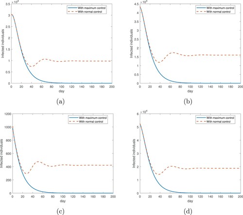2) )). Effectively, when the disease prevalence decreases, the transmission rates would increase due to weakened disease control. The results, represented by the red dashed lines in Figure 7, shows that the infection level would approach a positive endemic state over time. This is consistent with our analytical prediction given in Theorem A.2 in the Appendix. We also observe from Figure 7 that the simulated curves representing these two scenarios coincide during the first 30 days and then depart from each other afterwards, indicating that the impact of disease control measures at different strengths may be similar during the declining period of the outbreak, but the distinction would be reflected in the long run.

Figure 7. Long-term simulation (200 days starting from February 12, 2020) for the numbers of infected individuals in two scenarios: with maximum disease control (where each transmission rate is fixed at its minimum), and with normal disease control (where each transmission rate varies with the infection level and time). (a) Wuhan city; (b) Hubei province; (c) Guangdong province; (d) the entire country of China. The simulation is based on model (1(1) $\begin{array}{rl}\frac{\mathrm{d}S}{\mathrm{d}t}& =\mathrm{\Lambda }-{\beta }_E(I,t)SE-{\beta }_I(I,t)SI-{\beta }_V(I,t)SV-\mu S,\\ \frac{\mathrm{d}E}{\mathrm{d}t}& ={\beta }_E(I,t)SE+{\beta }_I(I,t)SI+{\beta }_V(I,t)SV-(\alpha +\mu )E,\\ \frac{\mathrm{d}I}{\mathrm{d}t}& =\alpha E-(w+\gamma +\mu )I,\\ \frac{\mathrm{d}R}{\mathrm{d}t}& =\gamma I-\mu R,\\ \frac{\mathrm{d}V}{\mathrm{d}t}& ={\xi }_{1}E+{\xi }_{2}I-\sigma V.\end{array}$(1) ) with both the direct and indirect transmission routes.

Finally, we present another set of fitting and simulation results to further demonstrate our model (1(1) $\begin{array}{rl}\frac{\mathrm{d}S}{\mathrm{d}t}& =\mathrm{\Lambda }-{\beta }_E(I,t)SE-{\beta }_I(I,t)SI-{\beta }_V(I,t)SV-\mu S,\\ \frac{\mathrm{d}E}{\mathrm{d}t}& ={\beta }_E(I,t)SE+{\beta }_I(I,t)SI+{\beta }_V(I,t)SV-(\alpha +\mu )E,\\ \frac{\mathrm{d}I}{\mathrm{d}t}& =\alpha E-(w+\gamma +\mu )I,\\ \frac{\mathrm{d}R}{\mathrm{d}t}& =\gamma I-\mu R,\\ \frac{\mathrm{d}V}{\mathrm{d}t}& ={\xi }_{1}E+{\xi }_{2}I-\sigma V.\end{array}$(1) ) with both the direct and indirect transmission routes. The accuracy of the reported COVID-19 data in China (as well as many other countries) has been under debate. In a recent Science article [11], the authors reported that about $86\mathrm{\%}$ of all infections in China were undocumented before January 23, 2020, and about $35\mathrm{\%}$ of all infections were undocumented afterwards. Using their estimated reporting rates which are constants in different time periods (i.e. 0.14 and 0.65 for reported new cases before and after January 23, respectively), we modify the numbers of COVID-19 cases in Wuhan city, Hubei and Guangdong provinces, and the entire country of China, and conduct data fitting and simulation again based on the same two-step procedure as described before. The results are presented in Table 5 and Figure 8. Despite the different datasets with elevated infection numbers, we observe similar patterns as those in Figures 1–6 at the city, province and country levels; the data fitting in the first time period (shown in Figure 8(a,c,e,g)) and the numerical simulation in the second time period (shown in Figure 8(b,d,f,h)) both agree well with the modified data. These results provide another piece of evidence for our model application, and indicate that the accuracy of the reported data does not have a significant impact on the validity of our methods.

Figure 8. Data fitting and simulation results based on the modified reported data using the reporting rates estimated in [11]: (a,b) Wuhan city; (c,d) Hubei province; (e,f) Guangdong province; (g,h) the entire country of China. Left panel: fitting from Jan 23 to Feb 11, 2020; Right panel: simulation from Feb 12 to May 1, 2020.

Table 5. Parameter estimates based on the modified reported data.

Location	Parameter	Fitting value	95% Confidence interval
Wuhan	${\xi }_1$	33.93	(28.438, 39.429)
	${\beta }_{V0}$	$1.44\times {10}^{-9}$	($1.260\times {10}^{-9}$, $1.624\times {10}^{-9}$)
	c	$1.25\times {10}^{-4}$	($1.114\times {10}^{-4}$, $1.388\times {10}^{-4}$)
Hubei	${\xi }_1$	90.56	(85.830, 95.299)
	${\beta }_{V0}$	$9.17\times {10}^{-11}$	($7.788\times {10}^{-11}$, $10.544\times {10}^{-11}$)
	c	$7.08\times {10}^{-5}$	($6.675\times {10}^{-5}$, $7.483\times {10}^{-5}$)
Guangdong	${\xi }_1$	83.73	(72.988, 94.472)
	${\beta }_{V0}$	$8.59\times {10}^{-11}$	($4.425\times {10}^{-11}$, $12.760\times {10}^{-11}$)
	c	$3.31\times {10}^{-3}$	($3.124\times {10}^{-3}$, $3.487\times {10}^{-3}$)
China	${\xi }_1$	43.80	(40.749, 46.849)
	${\beta }_{V0}$	$6.42\times {10}^{-12}$	($2.227\times {10}^{-12}$, $10.619\times {10}^{-12}$)
	c	$5.72\times {10}^{-5}$	($5.415\times {10}^{-5}$, $6.022\times {10}^{-5}$)

4. Discussion

Using a new mathematical model, we have performed a study on the transmission dynamics of COVID-19 in the city of Wuhan, the provinces of Hubei and Guangdong, and the entire country of China. Our model incorporates both the direct and indirect transmission routes, and emphasizes the role played by the environmental reservoirs in the transmission and spread of COVID-19. A unique feature of our model is that the transmission rates depend on the disease prevalence and time, with the potential to catch the realistic evolution of the contact pattern and transmission variation under the impact of the COVID-19 outbreak and the disease control measures.

Our numerical study consists of two major parts: the data fitting in the first time period (20 days from January 23 to February 11, 2020), and the simulation and prediction in the second time period (80 days from February 12 to May 1, 2020). The selection of February 12, 2020 to separate these two periods is based on several factors. First, after 20 days of implementing strong disease control measures ordered by the Chinese government, it is reasonable to assume that the disease transmission rates have been minimized and stabilized. Second, the change of the testing methods and criteria on February 12 led to a surge of confirmed cases in China, with an increase of about 14,000 new cases for Wuhan city alone in a single day. The spike in the reported data poses a potential difficulty for a curve fitting. Our approach overcomes this challenge by conducting data fitting up to February 11, 2020, and then using fixed transmission rates for the simulation and prediction afterwards. The results generated, particularly the good agreement between the simulation curves and the real data during the second time period at all the city, province and country levels, provide a validation of this approach. We have also compared the results with those obtained by removing the indirect transmission route from our model and using only the direct transmission routes for data fitting and simulation, and the comparison provides another validation of our approach. We have carried out the fitting and simulation tasks for both the publicly reported data and the modified data based on the estimated reporting rates from [11], and we observe very similar patterns.

The data fitting is employed to estimate the three key parameters ${\beta }_{V0}$, c and ${\xi }_1$ which are highly sensitive in our model. With their values fitted from the reported data, we are able to evaluate the basic reproduction number ${\mathcal{R}}_0$ at the city, province and country levels. In each of these calculations, we find that the component ${\mathcal{R}}_3$, which measures the risk of the environment-to-human transmission route, takes up a significant portion (ranging from $45\mathrm{\%}$ to $62\mathrm{\%}$) of ${\mathcal{R}}_0$. Furthermore, the simulation results in the second time period demonstrate that without incorporating the environmental transmission mode in our model, we would underestimate the severity and burden of the disease.

The ‘environment’ in this work is defined in a broad sense, including the air and all the surfaces and objects surrounding human individuals. The environment-to-human (or, indirect) transmission routes in our study include, but not limited to, all the fomite transmissions through contacting the contaminated surfaces and airborne transmissions through inhaling the floating coronavirus in the form of aerosols. Recent experimental findings, particularly in [22], provide clear evidences that coronaviruses can persist in these environmental settings from several hours to a few days, implying the risk of transmitting the pathogen from the environmental reservoirs to the human hosts. Our modeling study provides a quantification of this risk, and demonstrates that the environmental reservoirs indeed play an important role in shaping the COVID-19 epidemic in China. Our results provide a strong justification for the practice of hand washing and surface cleaning and disinfection, recommended by CDC and WHO, as these actions can effectively reduce the transmission of coronaviruses through the environment-to-human pathway.

Mathematical representation of the transmission rates for COVID-19 is certainly not unique, and our formulation in Equation (2(2) $\begin{array}{rl}{\beta }_E(I,t)& =\{\begin{array}{ll}{\beta }_{E0}{\mathrm{e}}^{-cI(t)},& 0\le t\le t^{\ast },\\ {\beta }_{E\ast },& t^{\ast }<t\le T,\end{array}\mathrm{where}{\beta }_{E\ast }={\beta }_{E0}{\mathrm{e}}^{-cI(t^{\ast })};\\ {\beta }_I(I,t)& =\{\begin{array}{ll}{\beta }_{I0}{\mathrm{e}}^{-cI(t)},& 0\le t\le t^{\ast },\\ {\beta }_{I\ast },& t^{\ast }<t\le T,\end{array}\mathrm{where}{\beta }_{I\ast }={\beta }_{I0}{\mathrm{e}}^{-cI(t^{\ast })};\\ {\beta }_V(I,t)& =\{\begin{array}{ll}{\beta }_{V0}{\mathrm{e}}^{-cI(t)},& 0\le t\le t^{\ast },\\ {\beta }_{V\ast },& t^{\ast }<t\le T,\end{array}\mathrm{where}{\beta }_{V\ast }={\beta }_{V0}{\mathrm{e}}^{-cI(t^{\ast })}.\end{array}$(2) ) provides a new and feasible way to characterize the temporal variation of the actual transmission rates under the impact of the epidemic evolution and the disease control measures, particularly for the outbreak period in China. Our numerical results demonstrate that this characterization, on which our two-step, data fitting and simulation, study approach is based, can well predict the epidemic development of COVID-19 in China from February 12 to May 1 in 2020. This pattern, though, does not necessarily reflect the reality for a long period of time.

The results presented in Figure 7 show that in the long run the curve with maximum disease control approaches 0 (the disease-free equilibrium), while the curve with normal disease control approaches a positive steady state (the endemic equilibrium). It is reasonable to expect that the realistic situation would find a way somewhere between these two hypothetical scenarios. Because relatively few new infections have appeared in China since early March of 2020, it is practically not meaningful to continue implementing control measures at the maximum strength. On the other hand, due to the severe consequence that COVID-19 has caused, many people would remain cautious in their behavior and attempt to reduce or limit their contact with others for a certain period of time. As a result, the practical transmission rates in the near future are expected to range between those associated with the two scenarios, and the real infection level would be bounded below by the disease-free state (determined by the maximum control) and above by the endemic state (determined by the normal control).

Acknowledgments

This work was partially supported by the National Institutes of Health under grant number 1R15GM131315. The authors are grateful to the two anonymous referees for their helpful comments that have improved the original manuscript.

Disclosure statement

No potential conflict of interest was reported by the author(s).

Additional information

Funding

This work was partially supported by the National Institutes of Health under grant number 1R15GM131315.

Appendix

A.1. Basic reproduction number

When restricted to the first time period, $0\le t\le t^{\ast }$, the model (1(1) $\begin{array}{rl}\frac{\mathrm{d}S}{\mathrm{d}t}& =\mathrm{\Lambda }-{\beta }_E(I,t)SE-{\beta }_I(I,t)SI-{\beta }_V(I,t)SV-\mu S,\\ \frac{\mathrm{d}E}{\mathrm{d}t}& ={\beta }_E(I,t)SE+{\beta }_I(I,t)SI+{\beta }_V(I,t)SV-(\alpha +\mu )E,\\ \frac{\mathrm{d}I}{\mathrm{d}t}& =\alpha E-(w+\gamma +\mu )I,\\ \frac{\mathrm{d}R}{\mathrm{d}t}& =\gamma I-\mu R,\\ \frac{\mathrm{d}V}{\mathrm{d}t}& ={\xi }_{1}E+{\xi }_{2}I-\sigma V.\end{array}$(1) ) is an autonomous system and its basic reproduction number can be computed using the standard next-generation matrix technique [21]. In this case we have ${\beta }_E(I,t)={\beta }_E(I)$, ${\beta }_I(I,t)={\beta }_I(I)$ and ${\beta }_V(I,t)={\beta }_V(I)$. The system (1(1) $\begin{array}{rl}\frac{\mathrm{d}S}{\mathrm{d}t}& =\mathrm{\Lambda }-{\beta }_E(I,t)SE-{\beta }_I(I,t)SI-{\beta }_V(I,t)SV-\mu S,\\ \frac{\mathrm{d}E}{\mathrm{d}t}& ={\beta }_E(I,t)SE+{\beta }_I(I,t)SI+{\beta }_V(I,t)SV-(\alpha +\mu )E,\\ \frac{\mathrm{d}I}{\mathrm{d}t}& =\alpha E-(w+\gamma +\mu )I,\\ \frac{\mathrm{d}R}{\mathrm{d}t}& =\gamma I-\mu R,\\ \frac{\mathrm{d}V}{\mathrm{d}t}& ={\xi }_{1}E+{\xi }_{2}I-\sigma V.\end{array}$(1) ) has a unique disease-free equilibrium (DFE) at (A1) $X_0=(S_0,E_0,I_0,R_0,V_0)=(\frac{\mathrm{\Lambda }}{\mu },0,0,0,0).$(A1) The infection components in this model are E, I and V. The new infection matrix F and the transition matrix V are given by (A2) $F=\left[\begin{array}{ccc}{\beta }_E(0)S_0& {\beta }_I(0)S_0& {\beta }_V(0)S_0\\ 0& 0& 0\\ 0& 0& 0\end{array}\right]\text{and}V=\left[\begin{array}{ccc}\alpha +\mu & 0& 0\\ -\alpha & w_1& 0\\ -{\xi }_1& -{\xi }_2& \sigma \end{array}\right],$(A2) where $w_1=w+\gamma +\mu$. The basic reproduction number of model (1(1) $\begin{array}{rl}\frac{\mathrm{d}S}{\mathrm{d}t}& =\mathrm{\Lambda }-{\beta }_E(I,t)SE-{\beta }_I(I,t)SI-{\beta }_V(I,t)SV-\mu S,\\ \frac{\mathrm{d}E}{\mathrm{d}t}& ={\beta }_E(I,t)SE+{\beta }_I(I,t)SI+{\beta }_V(I,t)SV-(\alpha +\mu )E,\\ \frac{\mathrm{d}I}{\mathrm{d}t}& =\alpha E-(w+\gamma +\mu )I,\\ \frac{\mathrm{d}R}{\mathrm{d}t}& =\gamma I-\mu R,\\ \frac{\mathrm{d}V}{\mathrm{d}t}& ={\xi }_{1}E+{\xi }_{2}I-\sigma V.\end{array}$(1) ) is then defined as the spectral radius of the next-generation matrix $F{V}^{-1}$ [21]; i.e. (A3) $\begin{array}{rl}{\mathcal{R}}_0=\rho (F{V}^{-1})& =\frac{{\beta }_E(0)S_0}{\alpha +\mu }+\frac{\alpha {\beta }_I(0)S_0}{w_1(\alpha +\mu )}+\frac{(w_1{\xi }_1+\alpha {\xi }_2){\beta }_V(0)S_0}{\sigma w_1(\alpha +\mu )},\\ & :={\mathcal{R}}_1+{\mathcal{R}}_2+{\mathcal{R}}_3,\end{array}$(A3) which provides a quantification of the potential for the coronavirus to invade the host population. The first two tems ${\mathcal{R}}_1$ and ${\mathcal{R}}_2$ come from the direct, human-to-human transmission routes, and the third term ${\mathcal{R}}_3$ indicates the contribution from the indirect, environment-to-human transmission route.

A.2. Parameter values

The values of the transmission constants ${\beta }_{E0}$ and ${\beta }_{I0}$ can be found in a recent study [17]. The incubation period of the infection ranges between 2–14 days, with a mean of 5–7 days [16]; we take the value of 7 days in our model. The average recovery period is about 15 days [16], and so we set the disease recovery rate as $\gamma =1/15$ per day. Members of the coronavirus family can survive in the environment from a few hours to several days [6,22], and we take the value of 1 day which results in a virus removal rate $\sigma =1$ per day. Meanwhile, since the Chinese government has been implementing a mandatory isolation policy and intense medical care for all the confirmed cases, represented by I in our model, the chance of those infected individuals spreading the coronavirus to the environment connected with the general public is extremely low, and so we assume the virus shedding rate from the infected individuals is zero; i.e. ${\xi }_2=0$. It turns out that the sensitivity of the parameter ${\xi }_2$ is also very low (see Section A.3). Additionally, the influx rate Λ depends on the location and population size. For example, the period of our concern starts on January 23, 2020, when the city of Wuhan was placed in quarantine and no one was allowed to move out of the city. Only a relatively small number of people (mainly public health professionals) travelled into the city since its lockdown. Thus, the influx rate for Wuhan city is mainly based on newborns and we obtain $\mathrm{\Lambda }=271.23$ per day [18]. Other parameter values are determined through data fitting.

A.3. Sensitivity analysis

The values of the three parameters ${\beta }_{V0}$, c and ${\xi }_1$ in our model are not available in the literature, and are thus estimated from data fitting. It turns out that these three are among the most sensitive parameters in all the model parameters. Below we provide details of our sensitivity analysis.

We consider the 9 parameters ${\beta }_{E0}$, ${\beta }_{I0}$, ${\beta }_{V0}$, c, α, w, γ, ${\xi }_1$ and ${\xi }_2$ in our model. We employ the basic differential equation analysis approach [5] to derive the sensitivity equations for our system (1(1) $\begin{array}{rl}\frac{\mathrm{d}S}{\mathrm{d}t}& =\mathrm{\Lambda }-{\beta }_E(I,t)SE-{\beta }_I(I,t)SI-{\beta }_V(I,t)SV-\mu S,\\ \frac{\mathrm{d}E}{\mathrm{d}t}& ={\beta }_E(I,t)SE+{\beta }_I(I,t)SI+{\beta }_V(I,t)SV-(\alpha +\mu )E,\\ \frac{\mathrm{d}I}{\mathrm{d}t}& =\alpha E-(w+\gamma +\mu )I,\\ \frac{\mathrm{d}R}{\mathrm{d}t}& =\gamma I-\mu R,\\ \frac{\mathrm{d}V}{\mathrm{d}t}& ={\xi }_{1}E+{\xi }_{2}I-\sigma V.\end{array}$(1) ). Let $\mathcal{X}=\{S,E,I,R,V\}$ and $P=\{{\beta }_{E0},{\beta }_{I0},{\beta }_{V0},c,\alpha ,w,\gamma ,{\xi }_1,{\xi }_2\}$. For $X\in \mathcal{X}$, $y\in P$, we define the relative sensitivity $s(X,y)$ of the state X to the parameter y, non-dimensionalized by the state X and the parameter value y, as (A4) $s(X,y)=\frac{\mathrm{\partial }X}{\mathrm{\partial }y}\frac{y}{X},X\ne 0.$(A4) To compute the partial derivative $\frac{\mathrm{\partial }X}{\mathrm{\partial }y}$, which is also referred to as a quasi-state variable, we differentiate it with respect to t to obtain (A5) $\frac{\mathrm{\partial }}{\mathrm{\partial }t}\left(\frac{\mathrm{\partial }X}{\mathrm{\partial }y}\right)=\frac{\mathrm{\partial }}{\mathrm{\partial }y}\left(\frac{\mathrm{\partial }X}{\mathrm{\partial }t}\right),X\in \mathcal{X},y\in P.$(A5) We then numerically solve for the quasi-state solutions $\{\frac{\mathrm{\partial }X}{\mathrm{\partial }y}:X\in \mathcal{X},y\in P\}$ by associating system (1(1) $\begin{array}{rl}\frac{\mathrm{d}S}{\mathrm{d}t}& =\mathrm{\Lambda }-{\beta }_E(I,t)SE-{\beta }_I(I,t)SI-{\beta }_V(I,t)SV-\mu S,\\ \frac{\mathrm{d}E}{\mathrm{d}t}& ={\beta }_E(I,t)SE+{\beta }_I(I,t)SI+{\beta }_V(I,t)SV-(\alpha +\mu )E,\\ \frac{\mathrm{d}I}{\mathrm{d}t}& =\alpha E-(w+\gamma +\mu )I,\\ \frac{\mathrm{d}R}{\mathrm{d}t}& =\gamma I-\mu R,\\ \frac{\mathrm{d}V}{\mathrm{d}t}& ={\xi }_{1}E+{\xi }_{2}I-\sigma V.\end{array}$(1) ) with system (A5(A5) $\frac{\mathrm{\partial }}{\mathrm{\partial }t}\left(\frac{\mathrm{\partial }X}{\mathrm{\partial }y}\right)=\frac{\mathrm{\partial }}{\mathrm{\partial }y}\left(\frac{\mathrm{\partial }X}{\mathrm{\partial }t}\right),X\in \mathcal{X},y\in P.$(A5) ).

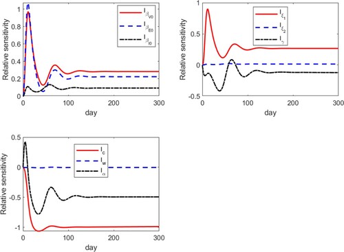
A typical set of results are presented in Figure A1, where we plot the relative sensitivities of I with respect to these 9 parameters in the set P, presented in three groups. We clearly observe that all these sensitivity variables approach a steady state in the long term. In particular, within each of the three groups, we have $\begin{array}{rl}& |s(I,{\beta }_{V0})|=0.234>max\{|s(I,{\beta }_{E0})|,|s(I,{\beta }_{I0})|\}=0.224,\\ & |s(I,c)|=0.987>max\{|s(I,w)|,|s(I,\alpha )|\}=0.492,\\ & |s(I,{\xi }_1)|=0.267>max\{|s(I,{\xi }_2)|,|s(I,\gamma )|\}=\mathrm{0.121.}\end{array}$Hence, we conclude that the three parameters ${\beta }_{V0}$, c and ${\xi }_1$ all have high sensitivities compared to other parameters. Meanwhile, we notice that the sensitivity of the parameter ${\xi }_2$ is extremely low, close to 0 all the time, which provides another justification of setting ${\xi }_2=0$ in our study.

Figure A1. The relative sensitivities $s(I,y)$ for the 9 parameters $y\in P$.

A.4. Equilibrium analysis

In this section, we conduct a mathematical analysis for the model (1(1) $\begin{array}{rl}\frac{\mathrm{d}S}{\mathrm{d}t}& =\mathrm{\Lambda }-{\beta }_E(I,t)SE-{\beta }_I(I,t)SI-{\beta }_V(I,t)SV-\mu S,\\ \frac{\mathrm{d}E}{\mathrm{d}t}& ={\beta }_E(I,t)SE+{\beta }_I(I,t)SI+{\beta }_V(I,t)SV-(\alpha +\mu )E,\\ \frac{\mathrm{d}I}{\mathrm{d}t}& =\alpha E-(w+\gamma +\mu )I,\\ \frac{\mathrm{d}R}{\mathrm{d}t}& =\gamma I-\mu R,\\ \frac{\mathrm{d}V}{\mathrm{d}t}& ={\xi }_{1}E+{\xi }_{2}I-\sigma V.\end{array}$(1) ) when ${\beta }_E(I,t)={\beta }_E(I)$, ${\beta }_I(I,t)={\beta }_I(I)$ and ${\beta }_V(I,t)={\beta }_V(I)$; i.e. when these transmission rates do not explicitly depend on time t. We focus our attention on the equilibria of the system (1(1) $\begin{array}{rl}\frac{\mathrm{d}S}{\mathrm{d}t}& =\mathrm{\Lambda }-{\beta }_E(I,t)SE-{\beta }_I(I,t)SI-{\beta }_V(I,t)SV-\mu S,\\ \frac{\mathrm{d}E}{\mathrm{d}t}& ={\beta }_E(I,t)SE+{\beta }_I(I,t)SI+{\beta }_V(I,t)SV-(\alpha +\mu )E,\\ \frac{\mathrm{d}I}{\mathrm{d}t}& =\alpha E-(w+\gamma +\mu )I,\\ \frac{\mathrm{d}R}{\mathrm{d}t}& =\gamma I-\mu R,\\ \frac{\mathrm{d}V}{\mathrm{d}t}& ={\xi }_{1}E+{\xi }_{2}I-\sigma V.\end{array}$(1) ) which will provide essential information regarding the long-term dynamics of the disease.

Let $(S,E,I,R,V)$ be an equilibrium of the system (1(1) $\begin{array}{rl}\frac{\mathrm{d}S}{\mathrm{d}t}& =\mathrm{\Lambda }-{\beta }_E(I,t)SE-{\beta }_I(I,t)SI-{\beta }_V(I,t)SV-\mu S,\\ \frac{\mathrm{d}E}{\mathrm{d}t}& ={\beta }_E(I,t)SE+{\beta }_I(I,t)SI+{\beta }_V(I,t)SV-(\alpha +\mu )E,\\ \frac{\mathrm{d}I}{\mathrm{d}t}& =\alpha E-(w+\gamma +\mu )I,\\ \frac{\mathrm{d}R}{\mathrm{d}t}& =\gamma I-\mu R,\\ \frac{\mathrm{d}V}{\mathrm{d}t}& ={\xi }_{1}E+{\xi }_{2}I-\sigma V.\end{array}$(1) ), which satisfies the following equations (A6) $\begin{array}{rl}& \mathrm{\Lambda }-{\beta }_E(I)SE-{\beta }_I(I)SI-{\beta }_V(I)SV-\mu S=0,\\ & {\beta }_E(I)SE+{\beta }_I(I)SI+{\beta }_V(I)SV-(\alpha +\mu )E=0,\\ & \alpha E-w_{1}I=0,\\ & \gamma I-\mu R=0,\\ & {\xi }_{1}E+{\xi }_{2}I-\sigma V=0.\end{array}$(A6) Solving (A6(A6) $\begin{array}{rl}& \mathrm{\Lambda }-{\beta }_E(I)SE-{\beta }_I(I)SI-{\beta }_V(I)SV-\mu S=0,\\ & {\beta }_E(I)SE+{\beta }_I(I)SI+{\beta }_V(I)SV-(\alpha +\mu )E=0,\\ & \alpha E-w_{1}I=0,\\ & \gamma I-\mu R=0,\\ & {\xi }_{1}E+{\xi }_{2}I-\sigma V=0.\end{array}$(A6) ) yields (A7) $\begin{array}{rl}S& ={\displaystyle \frac{1}{\mu }}(\mathrm{\Lambda }-(\alpha +\mu )E),\\ E& =\frac{w_1}{\alpha }I,\\ R& ={\displaystyle \frac{\gamma }{\mu }}I,\\ V& ={\displaystyle \frac{w_1{\xi }_1+\alpha {\xi }_2}{\sigma \alpha }}I.\end{array}$(A7) It follows from the first two equations of (A7(A7) $\begin{array}{rl}S& ={\displaystyle \frac{1}{\mu }}(\mathrm{\Lambda }-(\alpha +\mu )E),\\ E& =\frac{w_1}{\alpha }I,\\ R& ={\displaystyle \frac{\gamma }{\mu }}I,\\ V& ={\displaystyle \frac{w_1{\xi }_1+\alpha {\xi }_2}{\sigma \alpha }}I.\end{array}$(A7) ) that S can be denoted by a function of I, namely, (A8) $S=\varphi (I):={\displaystyle \frac{1}{\mu }}(\mathrm{\Lambda }-\frac{(\alpha +\mu )w_1}{\alpha }I).$(A8) Meanwhile, in view of the second equation of (A6(A6) $\begin{array}{rl}& \mathrm{\Lambda }-{\beta }_E(I)SE-{\beta }_I(I)SI-{\beta }_V(I)SV-\mu S=0,\\ & {\beta }_E(I)SE+{\beta }_I(I)SI+{\beta }_V(I)SV-(\alpha +\mu )E=0,\\ & \alpha E-w_{1}I=0,\\ & \gamma I-\mu R=0,\\ & {\xi }_{1}E+{\xi }_{2}I-\sigma V=0.\end{array}$(A6) ) and equations (A7(A7) $\begin{array}{rl}S& ={\displaystyle \frac{1}{\mu }}(\mathrm{\Lambda }-(\alpha +\mu )E),\\ E& =\frac{w_1}{\alpha }I,\\ R& ={\displaystyle \frac{\gamma }{\mu }}I,\\ V& ={\displaystyle \frac{w_1{\xi }_1+\alpha {\xi }_2}{\sigma \alpha }}I.\end{array}$(A7) ), we obtain (A9) $S=\psi (I):=(\alpha +\mu ){({\beta }_E(I)+\frac{\alpha }{w_1}{\beta }_I(I)+\frac{w_1{\xi }_1+\alpha {\xi }_2}{\sigma w_1}{\beta }_V(I))}^{-1}.$(A9) Let us now consider curves $S=\varphi (I),I\ge 0$ and $S=\psi (I),I\ge 0$. In particular, the intersections of these two curves in ${\mathbb{R}}_{+}^2$ determine the non-DFE equilibria. Clearly, $\varphi (I)$ is strictly decreasing, whereas $\psi (I)$ is increasing since ${\beta }_E(I),{\beta }_I(I)$, and ${\beta }_V(I)$ are nonnegative and decreasing functions of I. Additionally, one can easily verify that $\varphi (0)=S_0,\varphi (I_1)=0$, where $I_1=\frac{\alpha \mathrm{\Lambda }}{(\alpha +\mu )w_1}$, and $\psi (0)=(\alpha +\mu ){({\beta }_E(0)+\frac{\alpha }{w_1}{\beta }_I(0)+\frac{w_1{\xi }_1+\alpha {\xi }_2}{\sigma w_1}{\beta }_V(0))}^{-1}=\frac{S_0}{{\mathcal{R}}_0}.$Thus, we conclude:

1. If ${\mathcal{R}}_0>1$, these two curves have a unique intersection lying in the interior of ${\mathbb{R}}_{+}^2$, due to $\psi (0)<\varphi (0)$ and $\psi (I_1)\ge \psi (0)>0=\varphi (I_1)$. Furthermore, at this intersection point, Equation (A7(A7) $\begin{array}{rl}S& ={\displaystyle \frac{1}{\mu }}(\mathrm{\Lambda }-(\alpha +\mu )E),\\ E& =\frac{w_1}{\alpha }I,\\ R& ={\displaystyle \frac{\gamma }{\mu }}I,\\ V& ={\displaystyle \frac{w_1{\xi }_1+\alpha {\xi }_2}{\sigma \alpha }}I.\end{array}$(A7) ) yields a unique endemic equilibrium (EE) $X_{\ast }=(S_{\ast },E_{\ast },I_{\ast },R_{\ast },V_{\ast }).$

2. If ${\mathcal{R}}_0\le 1$, the two curves have no intersection in the interior of ${\mathbb{R}}_{+}^2$ as $\psi (0)\ge \varphi (0)$.

Therefore, by Equation (A7(A7) $\begin{array}{rl}S& ={\displaystyle \frac{1}{\mu }}(\mathrm{\Lambda }-(\alpha +\mu )E),\\ E& =\frac{w_1}{\alpha }I,\\ R& ={\displaystyle \frac{\gamma }{\mu }}I,\\ V& ={\displaystyle \frac{w_1{\xi }_1+\alpha {\xi }_2}{\sigma \alpha }}I.\end{array}$(A7) ), we find that the model (1(1) $\begin{array}{rl}\frac{\mathrm{d}S}{\mathrm{d}t}& =\mathrm{\Lambda }-{\beta }_E(I,t)SE-{\beta }_I(I,t)SI-{\beta }_V(I,t)SV-\mu S,\\ \frac{\mathrm{d}E}{\mathrm{d}t}& ={\beta }_E(I,t)SE+{\beta }_I(I,t)SI+{\beta }_V(I,t)SV-(\alpha +\mu )E,\\ \frac{\mathrm{d}I}{\mathrm{d}t}& =\alpha E-(w+\gamma +\mu )I,\\ \frac{\mathrm{d}R}{\mathrm{d}t}& =\gamma I-\mu R,\\ \frac{\mathrm{d}V}{\mathrm{d}t}& ={\xi }_{1}E+{\xi }_{2}I-\sigma V.\end{array}$(1) ) admits a unique equilibrium, the DFE $X_0$, if ${\mathcal{R}}_0\le 1$; and it admits two equilibria, the DFE $X_0$ and the EE $X_{\ast }$, if ${\mathcal{R}}_0>1$.

In what follows, we perform a study on the global stability of the DFE. By a simple comparison principle, we find that $0\le S+E+I+R\le S_0$ and $0\le V\le \frac{\xi S_0}{\sigma }$. Thus, it leads to a biologically feasible domain $\mathrm{\Omega }=\{(S,E,I,R,V)\in {\mathbb{R}}_{+}^5:S+E+I+R\le S_0,0\le V\le \frac{\xi S_0}{\sigma }\}.$

Theorem A.1

The following statements hold for the model (1(1) $\begin{array}{rl}\frac{\mathrm{d}S}{\mathrm{d}t}& =\mathrm{\Lambda }-{\beta }_E(I,t)SE-{\beta }_I(I,t)SI-{\beta }_V(I,t)SV-\mu S,\\ \frac{\mathrm{d}E}{\mathrm{d}t}& ={\beta }_E(I,t)SE+{\beta }_I(I,t)SI+{\beta }_V(I,t)SV-(\alpha +\mu )E,\\ \frac{\mathrm{d}I}{\mathrm{d}t}& =\alpha E-(w+\gamma +\mu )I,\\ \frac{\mathrm{d}R}{\mathrm{d}t}& =\gamma I-\mu R,\\ \frac{\mathrm{d}V}{\mathrm{d}t}& ={\xi }_{1}E+{\xi }_{2}I-\sigma V.\end{array}$(1) ).

(1)

If ${\mathcal{R}}_0\le 1$, the DFE of system (1(1) $\begin{array}{rl}\frac{\mathrm{d}S}{\mathrm{d}t}& =\mathrm{\Lambda }-{\beta }_E(I,t)SE-{\beta }_I(I,t)SI-{\beta }_V(I,t)SV-\mu S,\\ \frac{\mathrm{d}E}{\mathrm{d}t}& ={\beta }_E(I,t)SE+{\beta }_I(I,t)SI+{\beta }_V(I,t)SV-(\alpha +\mu )E,\\ \frac{\mathrm{d}I}{\mathrm{d}t}& =\alpha E-(w+\gamma +\mu )I,\\ \frac{\mathrm{d}R}{\mathrm{d}t}& =\gamma I-\mu R,\\ \frac{\mathrm{d}V}{\mathrm{d}t}& ={\xi }_{1}E+{\xi }_{2}I-\sigma V.\end{array}$(1) ) is globally asymptotically stable in Ω.

(2)

If ${\mathcal{R}}_0>1$, the DFE of system (1(1) $\begin{array}{rl}\frac{\mathrm{d}S}{\mathrm{d}t}& =\mathrm{\Lambda }-{\beta }_E(I,t)SE-{\beta }_I(I,t)SI-{\beta }_V(I,t)SV-\mu S,\\ \frac{\mathrm{d}E}{\mathrm{d}t}& ={\beta }_E(I,t)SE+{\beta }_I(I,t)SI+{\beta }_V(I,t)SV-(\alpha +\mu )E,\\ \frac{\mathrm{d}I}{\mathrm{d}t}& =\alpha E-(w+\gamma +\mu )I,\\ \frac{\mathrm{d}R}{\mathrm{d}t}& =\gamma I-\mu R,\\ \frac{\mathrm{d}V}{\mathrm{d}t}& ={\xi }_{1}E+{\xi }_{2}I-\sigma V.\end{array}$(1) ) is unstable and there exists a unique endemic equilibrium. Moreover, the disease is uniformly persistent in the interior of Ω, denoted by $\mathring{\mathrm{\Omega }}$; namely, $\underset{t\to \mathrm{\infty }}{lim inf}(E(t),I(t),V(t))>(\epsilon ,\epsilon ,\epsilon )$ for some $\epsilon >0$.

Proof.

Let $\mathbf{\text{X}}=(E,I,V{)}^T$. One can verify that ${\displaystyle \frac{\mathrm{d}\mathbf{\text{X}}}{\mathrm{d}t}}\le (F-V)\mathbf{\text{X}},$where the matrices F and V are given in Equation (A2(A2) $F=\left[\begin{array}{ccc}{\beta }_E(0)S_0& {\beta }_I(0)S_0& {\beta }_V(0)S_0\\ 0& 0& 0\\ 0& 0& 0\end{array}\right]\text{and}V=\left[\begin{array}{ccc}\alpha +\mu & 0& 0\\ -\alpha & w_1& 0\\ -{\xi }_1& -{\xi }_2& \sigma \end{array}\right],$(A2) ). By some algebraic manipulation, we let $\mathbf{\text{u}}=({\beta }_E(0),{\beta }_I(0),{\beta }_V(0)).$ It then follows from the fact ${\mathcal{R}}_0=\rho (F{V}^{-1})=\rho (V^{-1}F)$ and direct calculation that $\mathbf{\text{u}}$ is a left eigenvector associated with the eigenvalue ${\mathcal{R}}_0$ of the matrix $V^{-1}F$; i.e. $\mathbf{\text{u}}{V}^{-1}F={\mathcal{R}}_0\mathbf{\text{u}}$. Consider a Lyapunov function ${\mathcal{L}}_0=\mathbf{\text{u}}{V}^{-1}\mathbf{\text{X}}.$Differentiating $\mathcal{L}$ along the solutions of (1(1) $\begin{array}{rl}\frac{\mathrm{d}S}{\mathrm{d}t}& =\mathrm{\Lambda }-{\beta }_E(I,t)SE-{\beta }_I(I,t)SI-{\beta }_V(I,t)SV-\mu S,\\ \frac{\mathrm{d}E}{\mathrm{d}t}& ={\beta }_E(I,t)SE+{\beta }_I(I,t)SI+{\beta }_V(I,t)SV-(\alpha +\mu )E,\\ \frac{\mathrm{d}I}{\mathrm{d}t}& =\alpha E-(w+\gamma +\mu )I,\\ \frac{\mathrm{d}R}{\mathrm{d}t}& =\gamma I-\mu R,\\ \frac{\mathrm{d}V}{\mathrm{d}t}& ={\xi }_{1}E+{\xi }_{2}I-\sigma V.\end{array}$(1) ), we have (A10) $\frac{\mathrm{d}{\mathcal{L}}_0}{\mathrm{d}t}=\mathbf{\text{u}}{V}^{-1}{\displaystyle \frac{\mathrm{d}\mathbf{\text{X}}}{\mathrm{d}t}}\le \mathbf{\text{u}}{V}^{-1}(F-V)\mathbf{\text{X}}=\mathbf{\text{u}}({\mathcal{R}}_0-1)\mathbf{\text{X}}.$(A10) If ${\mathcal{R}}_0<1$, the equality $\frac{\mathrm{d}{\mathcal{L}}_0}{\mathrm{d}t}=0$ implies that $\mathbf{\text{u}}\mathbf{\text{X}}=0$. This leads to E = I = V = 0 by noting that all components of $\mathbf{\text{u}}$ are positive. Hence, when ${\mathcal{R}}_0<1$, equations of (A6(A6) $\begin{array}{rl}& \mathrm{\Lambda }-{\beta }_E(I)SE-{\beta }_I(I)SI-{\beta }_V(I)SV-\mu S=0,\\ & {\beta }_E(I)SE+{\beta }_I(I)SI+{\beta }_V(I)SV-(\alpha +\mu )E=0,\\ & \alpha E-w_{1}I=0,\\ & \gamma I-\mu R=0,\\ & {\xi }_{1}E+{\xi }_{2}I-\sigma V=0.\end{array}$(A6) ) yield $S=S_0$, and E = I = R = V = 0. Thus, the invariant set on which $\frac{\mathrm{d}{\mathcal{L}}_0}{\mathrm{d}t}=0$ contains only the point $X_0$.

If ${\mathcal{R}}_0=1$, then the equality $\frac{\mathrm{d}{\mathcal{L}}_0}{\mathrm{d}t}=0$ implies that $\begin{array}{rl}& (\frac{{\beta }_E(I)S}{S_0}+\frac{\alpha {\beta }_I(I)}{w_1}+\frac{(w_1{\xi }_1+\alpha {\xi }_2){\beta }_V(I)}{\sigma w_1}-\frac{\alpha +\mu }{S_0})E\\ & +(\frac{S}{S_0}{\beta }_I(I)-{\beta }_I(0))I+(\frac{S}{S_0}{\beta }_V(I)-{\beta }_V(0))V=0.\end{array}$It is easy to see that $\frac{S}{S_0}{\beta }_I(I)-{\beta }_I(0)\le 0,\frac{S}{S_0}{\beta }_V(I)-{\beta }_V(0)\le 0,$and $\begin{array}{rl}& \frac{{\beta }_E(I)S}{S_0}+\frac{\alpha {\beta }_I(I)}{w_1}+\frac{(w_1{\xi }_1+\alpha {\xi }_2){\beta }_V(I)}{\sigma w_1}-\frac{\alpha +\mu }{S_0}\\ & \le \frac{\alpha +\mu }{S_0}(\frac{{\beta }_E(0)S_0}{\alpha +\mu }+\frac{\alpha {\beta }_I(0)S_0}{w_1(\alpha +\mu )}+\frac{(w_1{\xi }_1+\alpha {\xi }_2){\beta }_V(0)S_0}{\sigma w_1(\alpha +\mu )}-1)\\ & =\frac{\alpha +\mu }{S_0}({\mathcal{R}}_0-1)=0.\end{array}$Hence, we have either E = I = V = 0, or ${\beta }_E(I)={\beta }_E(0),{\beta }_I(I)={\beta }_I(0),{\beta }_V(I)={\beta }_V(0)$, and $S=S_0$. As analyzed before, each case would indicate that the DEF $X_0$ is the only invariant set on $\{(S,E,I,R,V)\in \mathrm{\Omega }:\frac{\mathrm{d}{\mathcal{L}}_0}{\mathrm{d}t}=0\}$.

Therefore, when ${\mathcal{R}}_0<1$ or ${\mathcal{R}}_0=1$, the largest invariant set on which $\frac{\mathrm{d}{\mathcal{L}}_0}{\mathrm{d}t}=0$ consists of the singleton $X_0=(S_0,0,0,0,0)$. By LaSalle's Invariance Principle [10], the DFE is globally asymptotically stable in Ω if ${\mathcal{R}}_0\le 1$.

In contrast, if ${\mathcal{R}}_0>1$, then it follows from the continuity of vector fields that $\frac{\mathrm{d}{\mathcal{L}}_0}{\mathrm{d}t}>0$ in a neighbourhood of the DFE in $\mathring{\mathrm{\Omega }}$. Thus the DFE is unstable by the Lyapunov stability theory. The last part can be proved by the persistence theory [20].

Next, we analyze the stability of the endemic equilibrium. In order to simplify the notations, we adopt the abbreviations ${\beta }_E^{\ast }={\beta }_E(I_{\ast }),{\beta }_I^{\ast }={\beta }_I(I_{\ast }),{\beta }_V^{\ast }={\beta }_V(I_{\ast }),{\alpha }_{\mu }=\alpha +\mu .$

Theorem A.2

If ${\mathcal{R}}_0>1$, then the unique endemic equilibrium $X_{\ast }$ of the system (1(1) $\begin{array}{rl}\frac{\mathrm{d}S}{\mathrm{d}t}& =\mathrm{\Lambda }-{\beta }_E(I,t)SE-{\beta }_I(I,t)SI-{\beta }_V(I,t)SV-\mu S,\\ \frac{\mathrm{d}E}{\mathrm{d}t}& ={\beta }_E(I,t)SE+{\beta }_I(I,t)SI+{\beta }_V(I,t)SV-(\alpha +\mu )E,\\ \frac{\mathrm{d}I}{\mathrm{d}t}& =\alpha E-(w+\gamma +\mu )I,\\ \frac{\mathrm{d}R}{\mathrm{d}t}& =\gamma I-\mu R,\\ \frac{\mathrm{d}V}{\mathrm{d}t}& ={\xi }_{1}E+{\xi }_{2}I-\sigma V.\end{array}$(1) ) is locally asympototically stable.

Proof.

The Jacobian matrix of the system (1(1) $\begin{array}{rl}\frac{\mathrm{d}S}{\mathrm{d}t}& =\mathrm{\Lambda }-{\beta }_E(I,t)SE-{\beta }_I(I,t)SI-{\beta }_V(I,t)SV-\mu S,\\ \frac{\mathrm{d}E}{\mathrm{d}t}& ={\beta }_E(I,t)SE+{\beta }_I(I,t)SI+{\beta }_V(I,t)SV-(\alpha +\mu )E,\\ \frac{\mathrm{d}I}{\mathrm{d}t}& =\alpha E-(w+\gamma +\mu )I,\\ \frac{\mathrm{d}R}{\mathrm{d}t}& =\gamma I-\mu R,\\ \frac{\mathrm{d}V}{\mathrm{d}t}& ={\xi }_{1}E+{\xi }_{2}I-\sigma V.\end{array}$(1) ) at $X_{\ast }=(S_{\ast },E_{\ast },I_{\ast },R_{\ast },V_{\ast })$ is given by $J_{\ast }=\left[\begin{array}{ccccc}-{\displaystyle \frac{\mathrm{\Lambda }}{S_{\ast }}}& -{\beta }_E^{\ast }{S}_{\ast }& -\theta S_{\ast }& 0& -{\beta }_V^{\ast }{S}_{\ast }\\ {\displaystyle \frac{{\alpha }_{\mu }{E}_{\ast }}{S_{\ast }}}& -b{S}_{\ast }& {\theta }^{\ast }{S}_{\ast }& 0& {\beta }_V^{\ast }{S}_{\ast }\\ 0& \alpha & -w_1& 0& 0\\ 0& 0& \gamma & -\mu & 0\\ 0& {\xi }_1& {\xi }_2& 0& -\sigma \end{array}\right],$where $\theta ={\beta }_E^{\prime }(I_{\ast })E_{\ast }+{\beta }_V^{\prime }(I_{\ast })V_{\ast }+{\beta }_I^{\prime }(I_{\ast })I_{\ast }+{\beta }_I^{\ast }$ and $b=\frac{\alpha }{w_1}{\beta }_I^{\ast }+\frac{w_1{\xi }_1+\alpha {\xi }_2}{w_1\sigma }{\beta }_V^{\ast }$. The characteristic polynomial of $J_{\ast }$ is $f(\lambda )=(\lambda +\mu )({\lambda }^4+a_3{\lambda }^3+a_2{\lambda }^2+a_1\lambda +a_0),$where $\begin{array}{rl}{a}_3& =\frac{\mathrm{\Lambda }}{S_{\ast }}+b{S}_{\ast }+w_1+\sigma ,\\ a_2& =\frac{\mathrm{\Lambda }}{S_{\ast }}(b{S}_{\ast }+w_1+\sigma )+A{S}_{\ast }+w_1\sigma +{\alpha }_{\mu }{\beta }_E^{\ast }{E}_{\ast },\\ a_1& =\frac{\mathrm{\Lambda }\sigma w_1}{S_{\ast }}+S_{\ast }(\sigma B+\mu A)+{\alpha }_{\mu }{E}_{\ast }({\beta }_E^{\ast }+b)(w_1+\sigma ),\\ a_0& =\sigma w_1{\alpha }_{\mu }{E}_{\ast }({\beta }_E^{\ast }+b)+\mu S_{\ast }\sigma B,\\ A& =b(\sigma +w_1)-\alpha \theta -{\xi }_1{\beta }_V^{\ast },\\ B& =\alpha ({\beta }_I^{\ast }-\theta ).\end{array}$One can easily verify that $A\ge B\ge 0$, hence $a_3,a_2,a_1$, and $a_0$ are all positive. Note that $\mathrm{\Lambda }=\mu S_{\ast }+{\alpha }_{\mu }{E}_{\ast }$ and $(\sigma +w_1)(A-B)\ge \sigma w_{1}b$. We have $\begin{array}{rl}{a}_2{a}_3-a_1& >b{S}_{\ast }^{2}B+a_3(a_2-S_{\ast }B)-(a_1-S_{\ast }(\mu +\sigma )B)\\ & >b{S}_{\ast }^{2}B+\frac{{\mathrm{\Lambda }}^2}{S_{\ast }^2}(b{S}_{\ast }+w_1+\sigma )+b{S}_{\ast }(b\mathrm{\Lambda }+{\alpha }_{\mu }{\beta }_E^{\ast }{E}_{\ast }+w_1\sigma +(A-B)S_{\ast })\\ & +(w_1+\sigma )(b\mathrm{\Lambda }+\frac{\mathrm{\Lambda }}{S_{\ast }}(w_1+\sigma )+(A-B)S_{\ast }+w_1\sigma +b\mu S_{\ast })\\ & >0,\end{array}$and thereby, $\begin{array}{rl}& a_1(a_2{a}_3-a_1)=(S_{\ast }(\mu +\sigma )B+a_1-S_{\ast }(\mu +\sigma )B)(a_2{a}_3-a_1)\\ & =S_{\ast }(\mu +\sigma )B(a_2{a}_3-a_1)+(a_1-S_{\ast }(\mu +\sigma )B)(a_2{a}_3-a_1)\\ & >S_{\ast }(\mu +\sigma )B\{\frac{{\mathrm{\Lambda }}^2}{S_{\ast }^2}(b{S}_{\ast }+w_1+\sigma )+b^2{S}_{\ast }\mathrm{\Lambda }+(w_1+\sigma )(b\mathrm{\Lambda }+\frac{\mathrm{\Lambda }}{S_{\ast }}(w_1+\sigma )+b\mu S_{\ast })\}\\ & +\frac{\mathrm{\Lambda }\sigma w_1}{S_{\ast }}(a_2{a}_3-a_1)+{\alpha }_{\mu }{E}_{\ast }({\beta }_E^{\ast }+b)(w_1+\sigma )(a_2{a}_3-a_1)\\ & >S_{\ast }B\mu \sigma ({(\frac{\mathrm{\Lambda }}{S_{\ast }}+w_1+\sigma )}^2+b^2{S}_{\ast }^2+2b{S}_{\ast }(w_1+\sigma )+b\mathrm{\Lambda })+\mathrm{\Lambda }\sigma w_{1}b{S}_{\ast }B\\ & +{\alpha }_{\mu }{E}_{\ast }({\beta }_E^{\ast }+b)(w_1+\sigma )(a_2{a}_3-a_1)\\ & >S_{\ast }B\mu \sigma a_3^2+{\alpha }_{\mu }{E}_{\ast }({\beta }_E^{\ast }+b)(w_1+\sigma )\{\frac{{\mathrm{\Lambda }}^2}{S_{\ast }^2}(w_1+\sigma )+b{S}_{\ast }((A-B)S_{\ast }+w_1\sigma )\\ & +(w_1+\sigma )(b\mathrm{\Lambda }+\frac{\mathrm{\Lambda }}{S_{\ast }}(w_1+\sigma )+(A-B)S_{\ast }+w_1\sigma )\}\\ & >S_{\ast }B\mu \sigma a_3^2+\sigma w_1{\alpha }_{\mu }{E}_{\ast }({\beta }_E^{\ast }+b)a_3^2\\ & =a_0{a}_3^2.\end{array}$Thus, by Routh-Hurwitz stability criterion, $X_{\ast }$ is locally asymptotically stable.

Theorems A.1 and A.2 establish a sharp threshold at ${\mathcal{R}}_0=1$ for the disease dynamics: when ${\mathcal{R}}_0\le 1$, the infection will be eliminated and the disease-free state will be accomplished; when ${\mathcal{R}}_0>1$, the infection will persist and approach an endemic state in the long run. The results underscore the importance of reducing ${\mathcal{R}}_0$ below unity, through public health policies and outbreak control strategies, and through the control of both the direct and indirect transmission routes, in order to contain and eventually eradicate the disease.

Table A1. Definitions and values of model parameters.

Parameter	Definition	Estimated mean value	Source
Λ	Influx rate	271.23 per day	[18]
${\beta }_{E0}$	Transmission constant between S and E	$3.11\times {10}^{-8}$/person/day	[17]
${\beta }_{I0}$	Transmission constant between S and I	$0.62\times {10}^{-8}$/person/day	[17]
${\beta }_{V0}$	Transmission constant between S and V	fitting by data	–
c	Transmission adjustment coefficient	fitting by data	–
μ	Natural death rate	$3.01\times {10}^{-5}$ per day	[18]
$1/\alpha$	Incubation period	7 days	[16]
w	Disease-induced death rate	0.015 per day	[18]
γ	Recovery rate	1/15 per day	[16]
σ	Removal rate of virus	1 per day	[22]
${\xi }_1$	Virus shedding rate by exposed people	fitting by data	–
${\xi }_2$	Virus shedding rate by infected people	0 per person per day per ml	–

References

- Centers for disease control and prevention: Coronavirus (COVID-19). Available at https://www.cdc.gov/coronavirus/2019-ncov.
- J.F.-W. Chan, S. Yuan, K.-H. Kok, K.K.-K. To, H. Chu, J. Yang, F. Xing, J. Liu, C.C.-Y. Yip, R.W.-S. Poon, H.-W. Tsoi, S.K.-F. Lo, K.-H. Chan, V.K.-M. Poon, W.-M. Chan, J. Daniel Ip, J.-P.Cai, V.C.-C. Cheng, H. Chen, C.K.-M. Hui and K.-Y. Yuen, A familial cluster of pneumonia associated with the 2019 novel coronavirus indicating person-to-person transmission: A study of a family cluster, Lancet 395 (2020), pp. 514–523.
- Z.J. Cheng and J. Shan, 2019 novel coronavirus: Where we are and what we know, Infection 48 (2020), pp. 155–163.
- T. Ellerin, The new coronavirus: What we do – and don't – know, Harvard Health Blog, January 25, 2020. Available at https://www.health.harvard.edu/blog/the-new-coronavirus-what-we-do-and-dont-know-2020012518747.
- L. Ellwein, H. Tran, C. Zapata, V. Novak and M. Olufsen, Sensitivity analysis and model assessment: Mathematical models for arterial blood flow and blood pressure, Cardiovas. Eng. 8 (2008), pp. 94–108.
- C. Geller, M. Varbanov and R.E. Duval, Human coronaviruses: Insights into environmental resistance and its influence on the development of new antiseptic strategies, Viruses 4(11) (2012), pp. 3044–3068.
- L.E. Gralinski and V.D. Menachery, Return of the coronavirus: 2019-nCoV, Viruses 12(2) (2020), p. 135.
- N. Imai, A. Cori, I. Dorigatti, M. Baguelin, C.A. Donnelly, S. Riley and N.M. Ferguson, Report 3: Transmissibility of 2019-nCoV, published online January 25, 2020. Available at https://www.imperial.ac.uk/mrc-global-infectious-disease-analysis/news–wuhan-coronavirus/.
- G. Kampf, D. Todt, S. Pfaender and E. Steinmann, Persistence of coronaviruses on inanimate surfaces and its inactivation with biocidal agents, J. Hosp. Infect. 104(3) (2020), pp. 246–251.
- J.P. LaSalle, The Stability of Dynamical Systems, Regional Conference Series in Applied Mathematics, SIAM, Philadelphia, 1976.
- R. Li, S. Pei, B. Chen, Y. Song, T. Zhang, W. Yang and J. Shaman, Substantial undocumented infection facilitates the rapid dissemination of novel coronavirus (SARS-CoV2), Science 368 (2020), pp. 489–493.
- J. Lu, Z. Liu, V. Hill, M. Kang, H. Lin, J. Sun, N.R. Faria, J.T. McCrone, J. Peng, Q. Xiong, R. Yuan, L. Zeng, P. Zhou, C. Liang, L. Yi, J. Liu, J. Xiao, J. Hu, T. Liu, W. Ma, W. Li, J. Su, H. Zheng, B.Peng, S. Fang, W. Su, K. Li, R. Sun, R. Bai, X. Tang, M. Liang, J. Quick, T. Song, A. Rambaut, N.Loman, J. Raghwani, O.G. Pybus and C. Ke, Genomic epidemiology of SARS-CoV-2 in Guangdong province, China, Cell 181 (2020), pp. 997–1003.
- J.M. Read, J.R.E. Bridgen, D.A.T. Cummings, A. Ho and C.P. Jewell, Novel coronavirus 2019-nCoV: Early estimation of epidemiological parameters and epidemic predictions. Available at medRxiv https://doi.org/https://doi.org/10.1101/2020.01.23.20018549.
- C. Rothe, M. Schunk, P. Sothmann, G. Bretzel, G. Froeschl, C. Wallrauch, T. Zimmer, V. Thiel, C.Janke, W. Guggemos, M. Seilmaier, C. Drosten, P. Vollmar, K. Zwirglmaier and S. Zange, Transmission of 2019-nCoV infection from an asymptomatic contact in Germany, N. Engl. J. Med. 382 (2020), pp. 970–971.
- A.R. Sahin, A. Erdogan, P.M. Agaoglu, Y. Dineri, A.Y. Cakirci, M.E. Senel, R.A. Okyay and A.M.Tasdogan, 2019 novel coronavirus (COVID-19) outbreak: A review of the current literature, Eurasian J. Med. Oncol. 4(1) (2020), pp. 1–7.
- J.A. Spencer, D.P. Shutt, S.K.Moser, H. Clegg, H.J. Wearing, H. Mukundan and C.A. Manore, Epidemiological parameter review and comparative dynamics of influenza, respiratory syncytial virus, rhinovirus, human coronvirus, and adenovirus. Available at https://doi.org/https://doi.org/10.1101/2020.02.04.20020404.
- B. Tang, X. Wang, Q. Li, N.L. Bragazzi, S. Tang, Y. Xiao and J. Wu, Estimation of the transmission risk of 2019-nCoV and its implication for public health interventions, J. Clin. Med. 9(2) (2020), p. 462.
- The government of Wuhan. Available at http://english.wh.gov.cn
- The health commission of Hubei province. Available from http://wjw.hubei.gov.cn/fbjd/dtyw/index_16.shtml
- H.R. Thieme, Persistence under relaxed point-dissipativity (with application to an endemic model), SIAM J. Math. Anal. 24 (1993), pp. 407–435.
- P. van den Driessche and J. Watmough, Reproduction numbers and sub-threshold endemic equilibria for compartmental models of disease transmission, Math. Biosci. 180 (2002), pp. 29–48.
- N. van Doremalen, T. Bushmaker, D.H. Morris, M.G. Holbrook, A. Gamble, B.N. Williamson, A.Tamin, J.L. Harcourt, N.J. Thornburg, S.I. Gerber, J.O. Lloyd-Smith, E. de Wit and V.J. Munster, Aerosol and surface stability of SARS-CoV-2 as compared with SARS-CoV-1, N. Engl. J. Med. 382 (2020), pp. 1564–1567.
- J. Wang, Mathematical models for COVID-19: Applications, limitations, and potentials, J. Public Health Emerg. 4 (2020), p. 9.
- J.-T. Wu, K. Leung and G.M. Leung, Nowcasting and forecasting the potential domestic and international spread of the 2019-nCoV outbreak originating in Wuhan, China: a modelling study, Lancet 395 (2020), pp. 689–697.
- C. Yang and J. Wang, A mathematical model for the novel coronavirus epidemic in Wuhan, China, Math. Biosci. Eng. 17(3) (2020), pp. 2708–2724.
- C. Yang, X. Wang, D. Gao and J. Wang, Impact of awareness programs on cholera dynamics: Two modeling approaches, Bull. Math. Biol. 79(9) (2017), pp. 2109–2131.
- C. Yeo, S. Kaushal and D. Yeo, Enteric involvement of coronaviruses: is faecal-oral transmission of SARS-CoV-2 possible? Lancet Gastroenterol. Hepatol. 5(4) (2020), pp. 335–337.
- H. Zhong and W. Wang, Mathematical analysis for COVID-19 resurgence in the contaminated environment, Math. Biosci. Eng. 17(6) (2020), pp. 6909–6927.