Impulsive release strategies of sterile mosquitos for optimal control of wild population

Abstract

To investigate the release strategies of sterile mosquitoes for the wild population control, we propose mathematical models for the interaction between two-mosquito populations incorporating impulsive releases of sterile ones. The long-term control model is first studied, and the existence and stability of the wild mosquito-extinction periodic solution are exploited. Thresholds of the release amount and release period which can guarantee the elimination of the wild mosquitos are obtained. Then for the limited-time control model, three different optimal strategies in impulsive control are investigated. By applying a time rescaling technique and an optimization algorithm based on gradient, the optimal impulsive release timings and amounts of sterile mosquitoes are obtained. Our results show that the optimal selection of release timing is more important than the optimal selection of release amount, while mixed optimal control has the best comprehensive effect.

KEYWORDS:

• Optimal control
• impulsive releases
• release timing
• release amount

2010 MATHEMATICS SUBJECT CLASSIFICATIONS:

• 92D25
• 92D40
• 34C60

1. Introduction

The sterile insect technique (SIT)-which can reduce mating between fertile wild counterparts by releasing artificially reared sterilized males into field, has been widely applied to control insect pests of agriculture [3–7]. With the breakthrough in rearing methods [19], SIT in recent decades starts to be used against mosquitoes for the mosquito-borne disease control [1,2,10–14,17,18,20,24,29,30,40]. SIT is an environment-friendly method which can disrupt the natural breeding of wild mosquitoes by preventing them from producing viable offspring. Then through reasonable sterile mosquito releases, people may eventually wipe out the wild ones in a field.

For the release strategy of sterile mosquitoes, a lot of research work has been done. K. R. Fister et al. in [16] proposed an optimal control framework to exploit the effect of sterile mosquito releases in reducing the incidence of mosquito-borne diseases. S. M. White et al. explored the mechanism of how an insect fitness cost affects different control policies by constructing a stage-structured mathematical model for the mosquito Aedes aegypti in [32]. J. Li and his partners in [22] investigated multiple policies of sterile mosquito release by formulating discrete dynamical systems for the interaction between two mosquito populations. While L. Cai et al. in [12] studied the impact of the SIT on disease transmission by constructing continuous dynamical systems incorporating constant, proportional and Holling-II type release rates. In view of that larvae and adult mosquitoes have distinct responses to the density-dependent factor, J. Li formulated several dynamical systems with stage structure and different release policies to discuss the application of SIT in the control of mosquito-borne diseases [20]. Multiple sterile males release techniques aiming at reduction and even elimination of mosquito populations are studied in [30] and [10], while [18] and [13] mainly investigated the bifurcation phenomenon of two mathematical models involving different releases.

Obviously, the release process is relatively instantaneous with respect to the population development, and it is often the case that people need release sterile mosquitoes several times to control the population level of the wild ones. Based on these facts, Several studies related to impulsive SIT mosquito control have been done [2,10,11,14,17,30] and also reference there in). They proposed mathematical models and studied different kinds of release strategies: periodic impulsive releases and state feedback impulsive releases. In particular, P. A. Bliman et al. in [10] studied the periodic impulsive releases under open-loop control, state feedback impulsive releases under closed-loop control and a mixed release strategy that combines open-loop and closed-loop controls.

In addition to the classic SIT, the Wolbachia driven mosquito control technique is also used in the laboratory or field. For example, J. Yu in [34] introduced a model of differential equations with a time delay to study the suppression dynamics of wild mosquitoes intervened by the releasing of Wolbachia-infected males. Unlike many studies, the population suppression in this work tried to avoid releasing infected females, just released living infected males, and aimed for eliminating the whole population of mosquitoes. Then J. Yu, J. Li and their partners introduced the sexual lifespan of sterile mosquitoes and assumed that the interaction happens only when the sterile mosquitoes are still sexually active [21,35–37]). They investigated the impact of the sexual lifespan of sterile mosquitoes on mosquito population suppression based on delay differential equations and gave a lot of important results. J. Yu and B. Zheng in [38] specially studied Wolbachia persistence by extra releases of Wolbachia-infected mosquitoes and obtained a maximal maternal leakage rate threshold such that infected mosquitoes can persist.

However, the artificial rearing and release of sterile mosquitoes has a very real financial price. Thus, for the wild mosquito control, we should consider both the control effect and the economic input. For this reason, optimal control incorporating economic input is a better choice. The authors in [1] studied the optimal release strategies in order to maximize the efficiency of SIT based on a continuous dynamic system. While in [11], SIT-control intervention programs are designed to avoid the real-time monitoring of the wild population and require to mass-rear a minimal overall number of sterile insects, which provided an experience for periodic impulsive releases.

Lots of biological control methodologies have been used in the optimal impulsive management of population [15,16,22,26,33,39]). X. Y. Liang et al. studied an eco-epidemiological model with pulse interferences, and investigated several optimal strategies in impulsive control [25]. While Y. Z. Pei et al. exploited an optimal pest management system incorporating impulsive human interventions and residual effect of pesticides [28]. In this study, we propose a stage-structured population model for the development of wild mosquitos incorporating impulsive deliveries of reared sterile ones, and then study the long-term control and limited-time optimal control of wild mosquitoes by adjusting release amount and release timing of sterile mosquitoes.

The paper is structured as follows: In Section 2, we construct a model for the long-term control of wild mosquitoes with periodic impulsive releases of sterile ones and study its dynamical properties. In Section 3, we extend the long-term control model and raise a limited-time optimal control problem. Three kinds of optimal strategies in impulsive control aiming at minimizing the amount of wild mosquitoes and the economic cost are discussed. By applying a time rescaling technology, we present the gradient expressions of the cost function with respect to control parameters. Then optimal release timing and release amount are gained by numerical simulations in Section 4. Finally, we finish this paper with a brief conclusion in Section 5.

2. Long-term control with periodic impulsive releases

2.1. Model formulation

The basic ODE model studied in this paper is the following stage-structured interactive system of two-mosquito populations (see [24] and [20]) (1) $\left\{\begin{array}{l}\frac{\mathrm{d}J\left(t\right)}{\mathrm{d}t}=\frac{rA\left(t\right)}{A\left(t\right)+g\left(t\right)}A\left(t\right)-\frac{\alpha J\left(t\right)}{1+J\left(t\right)}-(d_0+d_{1}J(t\left)\right)J\left(t\right),\\ \frac{\mathrm{d}A\left(t\right)}{\mathrm{d}t}=\frac{\alpha J\left(t\right)}{1+J\left(t\right)}-{\mu }_{1}A\left(t\right),\\ \frac{\mathrm{d}g\left(t\right)}{\mathrm{d}t}=B(\cdot )-{\mu }_{2}g\left(t\right)\end{array}\right.$(1) where $J\left(t\right),A\left(t\right)$ are the numbers of the larvae and the adults of wild mosquitoes at t respectively, while $g\left(t\right)$ is the number of the sterile ones. $r=\overline{r}\overline{s}$, where $\overline{r}$ represents the average number of wild offspring that a mosquito can produce per day and $\overline{s}$ is the sex-ratio of the mosquito population. $\frac{\alpha J}{1+J}$ is the emergence rate from larvae to adults, and $d_0+d_{1}J\left(t\right)$ stands for the death rate of larvae incorporating density restriction, while ${\mu }_1,{\mu }_2$ denote death rates of adult wild mosquitoes and sterile ones, respectively. $B(\cdot )$ stands for the release rate of sterile mosquitoes. Since the sex-structure of wild mosquitoes is ignored in this work, we assume that the number of living female mosquitoes is equal to the number of living male mosquitoes at each moment t.

Different from [24] and [20], we consider the rate of emergence from larvae to adults to be a function of the larvae J, denoted by $\kappa \left(J\right)>0$, satisfying $\kappa \left(0\right)=0$, ${\kappa }^{\prime }\left(J\right)\ge 0$ and ${\kappa }^{″}\left(J\right)\le 0$. We then assume that κ is approximately proportional to J when J is small, and as the size of the larvae becomes sufficiently large, duo to the intraspecific competition, the emergence saturates. After J reaches a threshold size, it is relatively close to a constant determined by this threshold. Thus we assume the emergence rate has the form $\kappa \left(J\right)=\frac{\alpha J}{\gamma +J}$.

We now extend the above model and convert the continuous release form $B(\cdot )$ to an impulsive one, then a new interaction model of two-mosquito populations incorporating periodic impulsive human intervention is proposed as follows: (2) $\left\{\begin{array}{l}\left.\begin{array}{l}\frac{\mathrm{d}J\left(t\right)}{\mathrm{d}t}=\frac{rA\left(t\right)}{A\left(t\right)+g\left(t\right)}A\left(t\right)-\frac{\alpha J\left(t\right)}{\gamma +J\left(t\right)}\\ -(d_0+d_{1}J(t\left)\right)J\left(t\right),\\ \frac{\mathrm{d}A\left(t\right)}{\mathrm{d}t}=\frac{\alpha J\left(t\right)}{\gamma +J\left(t\right)}-{\mu }_{1}A\left(t\right),\\ \frac{\mathrm{d}g\left(t\right)}{\mathrm{d}t}=-{\mu }_{2}g\left(t\right),\end{array}\right\}t\ne kp,k=1,2,\dots ,\\ \left.\begin{array}{l}J\left(t^{+}\right)=J\left(t\right),\\ A\left(t^{+}\right)=A\left(t\right),\\ g\left(t^{+}\right)=g\left(t\right)+\sigma ,\end{array}\right\}t=kp\end{array}\right.$(2) with $J\left(0\right)=J_0>0,A\left(0\right)=A_0>0$ and $g\left(0\right)=g_0>0$. p is the release period while σ is the amount released each time.

In the following, we focus on dynamical properties of the system (2(2) $\left\{\begin{array}{l}\left.\begin{array}{l}\frac{\mathrm{d}J\left(t\right)}{\mathrm{d}t}=\frac{rA\left(t\right)}{A\left(t\right)+g\left(t\right)}A\left(t\right)-\frac{\alpha J\left(t\right)}{\gamma +J\left(t\right)}\\ -(d_0+d_{1}J(t\left)\right)J\left(t\right),\\ \frac{\mathrm{d}A\left(t\right)}{\mathrm{d}t}=\frac{\alpha J\left(t\right)}{\gamma +J\left(t\right)}-{\mu }_{1}A\left(t\right),\\ \frac{\mathrm{d}g\left(t\right)}{\mathrm{d}t}=-{\mu }_{2}g\left(t\right),\end{array}\right\}t\ne kp,k=1,2,\dots ,\\ \left.\begin{array}{l}J\left(t^{+}\right)=J\left(t\right),\\ A\left(t^{+}\right)=A\left(t\right),\\ g\left(t^{+}\right)=g\left(t\right)+\sigma ,\end{array}\right\}t=kp\end{array}\right.$(2) ), and investigate the release strategy for the long-term control of wild mosquitoes theoretically and numerically.

2.2. Dynamics analysis

We firstly discuss the existence of the boundary periodic solution (wild mosquito eradication) of system (2(2) $\left\{\begin{array}{l}\left.\begin{array}{l}\frac{\mathrm{d}J\left(t\right)}{\mathrm{d}t}=\frac{rA\left(t\right)}{A\left(t\right)+g\left(t\right)}A\left(t\right)-\frac{\alpha J\left(t\right)}{\gamma +J\left(t\right)}\\ -(d_0+d_{1}J(t\left)\right)J\left(t\right),\\ \frac{\mathrm{d}A\left(t\right)}{\mathrm{d}t}=\frac{\alpha J\left(t\right)}{\gamma +J\left(t\right)}-{\mu }_{1}A\left(t\right),\\ \frac{\mathrm{d}g\left(t\right)}{\mathrm{d}t}=-{\mu }_{2}g\left(t\right),\end{array}\right\}t\ne kp,k=1,2,\dots ,\\ \left.\begin{array}{l}J\left(t^{+}\right)=J\left(t\right),\\ A\left(t^{+}\right)=A\left(t\right),\\ g\left(t^{+}\right)=g\left(t\right)+\sigma ,\end{array}\right\}t=kp\end{array}\right.$(2) ), then obtain conditions under which it is globally asymptotically stable. On basis of this, theoretical and practical methods are provided to select the release amount σ and the release period p so that the wild mosquito population can be eliminated.

Suppose $X\left(t\right)=\left(J\right(t),A(t),g(t){)}^T$ is an arbitrary solution of (2(2) $\left\{\begin{array}{l}\left.\begin{array}{l}\frac{\mathrm{d}J\left(t\right)}{\mathrm{d}t}=\frac{rA\left(t\right)}{A\left(t\right)+g\left(t\right)}A\left(t\right)-\frac{\alpha J\left(t\right)}{\gamma +J\left(t\right)}\\ -(d_0+d_{1}J(t\left)\right)J\left(t\right),\\ \frac{\mathrm{d}A\left(t\right)}{\mathrm{d}t}=\frac{\alpha J\left(t\right)}{\gamma +J\left(t\right)}-{\mu }_{1}A\left(t\right),\\ \frac{\mathrm{d}g\left(t\right)}{\mathrm{d}t}=-{\mu }_{2}g\left(t\right),\end{array}\right\}t\ne kp,k=1,2,\dots ,\\ \left.\begin{array}{l}J\left(t^{+}\right)=J\left(t\right),\\ A\left(t^{+}\right)=A\left(t\right),\\ g\left(t^{+}\right)=g\left(t\right)+\sigma ,\end{array}\right\}t=kp\end{array}\right.$(2) ). We can obtain easily that $X\left(t\right)$ is continuous between every two adjacent pulses and $X\left(k{p}^{+}\right)={\displaystyle \underset{ϵ\to 0^{+}}{lim}X(kp+ϵ)}$ exists. Then the existence and uniqueness of solutions of (2(2) $\left\{\begin{array}{l}\left.\begin{array}{l}\frac{\mathrm{d}J\left(t\right)}{\mathrm{d}t}=\frac{rA\left(t\right)}{A\left(t\right)+g\left(t\right)}A\left(t\right)-\frac{\alpha J\left(t\right)}{\gamma +J\left(t\right)}\\ -(d_0+d_{1}J(t\left)\right)J\left(t\right),\\ \frac{\mathrm{d}A\left(t\right)}{\mathrm{d}t}=\frac{\alpha J\left(t\right)}{\gamma +J\left(t\right)}-{\mu }_{1}A\left(t\right),\\ \frac{\mathrm{d}g\left(t\right)}{\mathrm{d}t}=-{\mu }_{2}g\left(t\right),\end{array}\right\}t\ne kp,k=1,2,\dots ,\\ \left.\begin{array}{l}J\left(t^{+}\right)=J\left(t\right),\\ A\left(t^{+}\right)=A\left(t\right),\\ g\left(t^{+}\right)=g\left(t\right)+\sigma ,\end{array}\right\}t=kp\end{array}\right.$(2) ) is guaranteed for the smooth properties of functions in the first three equations [8,9].

Firstly, we investigate the positivity and boundedness of the solution of system (2(2) $\left\{\begin{array}{l}\left.\begin{array}{l}\frac{\mathrm{d}J\left(t\right)}{\mathrm{d}t}=\frac{rA\left(t\right)}{A\left(t\right)+g\left(t\right)}A\left(t\right)-\frac{\alpha J\left(t\right)}{\gamma +J\left(t\right)}\\ -(d_0+d_{1}J(t\left)\right)J\left(t\right),\\ \frac{\mathrm{d}A\left(t\right)}{\mathrm{d}t}=\frac{\alpha J\left(t\right)}{\gamma +J\left(t\right)}-{\mu }_{1}A\left(t\right),\\ \frac{\mathrm{d}g\left(t\right)}{\mathrm{d}t}=-{\mu }_{2}g\left(t\right),\end{array}\right\}t\ne kp,k=1,2,\dots ,\\ \left.\begin{array}{l}J\left(t^{+}\right)=J\left(t\right),\\ A\left(t^{+}\right)=A\left(t\right),\\ g\left(t^{+}\right)=g\left(t\right)+\sigma ,\end{array}\right\}t=kp\end{array}\right.$(2) ).

Proposition 2.1

Solutions of system (2(2) $\left\{\begin{array}{l}\left.\begin{array}{l}\frac{\mathrm{d}J\left(t\right)}{\mathrm{d}t}=\frac{rA\left(t\right)}{A\left(t\right)+g\left(t\right)}A\left(t\right)-\frac{\alpha J\left(t\right)}{\gamma +J\left(t\right)}\\ -(d_0+d_{1}J(t\left)\right)J\left(t\right),\\ \frac{\mathrm{d}A\left(t\right)}{\mathrm{d}t}=\frac{\alpha J\left(t\right)}{\gamma +J\left(t\right)}-{\mu }_{1}A\left(t\right),\\ \frac{\mathrm{d}g\left(t\right)}{\mathrm{d}t}=-{\mu }_{2}g\left(t\right),\end{array}\right\}t\ne kp,k=1,2,\dots ,\\ \left.\begin{array}{l}J\left(t^{+}\right)=J\left(t\right),\\ A\left(t^{+}\right)=A\left(t\right),\\ g\left(t^{+}\right)=g\left(t\right)+\sigma ,\end{array}\right\}t=kp\end{array}\right.$(2) ) with non-negative initial conditions are always non-negative.

Proof.

Let $\left(J\right(t),A(t),g(t\left)\right)$ be a solution of (2(2) $\left\{\begin{array}{l}\left.\begin{array}{l}\frac{\mathrm{d}J\left(t\right)}{\mathrm{d}t}=\frac{rA\left(t\right)}{A\left(t\right)+g\left(t\right)}A\left(t\right)-\frac{\alpha J\left(t\right)}{\gamma +J\left(t\right)}\\ -(d_0+d_{1}J(t\left)\right)J\left(t\right),\\ \frac{\mathrm{d}A\left(t\right)}{\mathrm{d}t}=\frac{\alpha J\left(t\right)}{\gamma +J\left(t\right)}-{\mu }_{1}A\left(t\right),\\ \frac{\mathrm{d}g\left(t\right)}{\mathrm{d}t}=-{\mu }_{2}g\left(t\right),\end{array}\right\}t\ne kp,k=1,2,\dots ,\\ \left.\begin{array}{l}J\left(t^{+}\right)=J\left(t\right),\\ A\left(t^{+}\right)=A\left(t\right),\\ g\left(t^{+}\right)=g\left(t\right)+\sigma ,\end{array}\right\}t=kp\end{array}\right.$(2) ) with non-negative initial conditions. Obviously, we have $dg\left(t\right)/\mathrm{d}t=0$ if $g\left(t\right)=0$, then we can get $g\left(t\right)>0$, $t\ge 0$ for $g\left(0\right)>0$.

Assume there exists t>0 satisfying $A\left(t\right)<0$, and we denote $\tilde{t}=inf\{t:A(t)<0\}$, then $A\left(\tilde{t}\right)=0$ and $A^{\prime }\left(\tilde{t}\right)\le 0$. Substitute them into the second equation of (2(2) $\left\{\begin{array}{l}\left.\begin{array}{l}\frac{\mathrm{d}J\left(t\right)}{\mathrm{d}t}=\frac{rA\left(t\right)}{A\left(t\right)+g\left(t\right)}A\left(t\right)-\frac{\alpha J\left(t\right)}{\gamma +J\left(t\right)}\\ -(d_0+d_{1}J(t\left)\right)J\left(t\right),\\ \frac{\mathrm{d}A\left(t\right)}{\mathrm{d}t}=\frac{\alpha J\left(t\right)}{\gamma +J\left(t\right)}-{\mu }_{1}A\left(t\right),\\ \frac{\mathrm{d}g\left(t\right)}{\mathrm{d}t}=-{\mu }_{2}g\left(t\right),\end{array}\right\}t\ne kp,k=1,2,\dots ,\\ \left.\begin{array}{l}J\left(t^{+}\right)=J\left(t\right),\\ A\left(t^{+}\right)=A\left(t\right),\\ g\left(t^{+}\right)=g\left(t\right)+\sigma ,\end{array}\right\}t=kp\end{array}\right.$(2) ), then we obtain $A^{\prime }\left(\tilde{t}\right)=\frac{\alpha J\left(\tilde{t}\right)}{\gamma +J\left(\tilde{t}\right)}\le 0$.

If $J\left(t\right)$ is non-negative for t>0, then $J\left(\tilde{t}\right)\ge 0$ and we get $A^{\prime }\left(\tilde{t}\right)\ge 0$. It follows from $A^{\prime }\left(\tilde{t}\right)\le 0$ that $A^{\prime }\left(\tilde{t}\right)=0$, then we have $A^{\prime }\left(\tilde{t}\right)=A\left(\tilde{t}\right)=J\left(\tilde{t}\right)=J^{\prime }\left(\tilde{t}\right)=0$. According to the definition of $\tilde{t}$, there must be a sufficiently small constant ${ϵ}_1>0$ such that $A(\tilde{t}+{ϵ}_1)<0,A^{\prime }(\tilde{t}+{ϵ}_1)<0$ and $J(\tilde{t}+{ϵ}_1)\ge 0$. Therefore $A^{\prime }(\tilde{t}+{ϵ}_1)=\frac{\alpha J(\tilde{t}+{ϵ}_1)}{\gamma +J(\tilde{t}+{ϵ}_1)}-{\mu }_{1}A(\tilde{t}+{ϵ}_1)>0$, which leads to a contradiction.

If there exists t>0 satisfying $J\left(t\right)<0$, we denote $\overline{t}=inf\{t:J(t)<0\}$, then $J\left(\overline{t}\right)=0$ and $J^{\prime }\left(\overline{t}\right)\le 0$. Substitute them into the first equation of (2(2) $\left\{\begin{array}{l}\left.\begin{array}{l}\frac{\mathrm{d}J\left(t\right)}{\mathrm{d}t}=\frac{rA\left(t\right)}{A\left(t\right)+g\left(t\right)}A\left(t\right)-\frac{\alpha J\left(t\right)}{\gamma +J\left(t\right)}\\ -(d_0+d_{1}J(t\left)\right)J\left(t\right),\\ \frac{\mathrm{d}A\left(t\right)}{\mathrm{d}t}=\frac{\alpha J\left(t\right)}{\gamma +J\left(t\right)}-{\mu }_{1}A\left(t\right),\\ \frac{\mathrm{d}g\left(t\right)}{\mathrm{d}t}=-{\mu }_{2}g\left(t\right),\end{array}\right\}t\ne kp,k=1,2,\dots ,\\ \left.\begin{array}{l}J\left(t^{+}\right)=J\left(t\right),\\ A\left(t^{+}\right)=A\left(t\right),\\ g\left(t^{+}\right)=g\left(t\right)+\sigma ,\end{array}\right\}t=kp\end{array}\right.$(2) ), and we get $J^{\prime }\left(\overline{t}\right)=\frac{r{A}^2\left(\overline{t}\right)}{A\left(\overline{t}\right)+g\left(\overline{t}\right)}\le 0.$

Then we need discuss the following three cases:

1. $\tilde{t}=\overline{t}$. There is $A^{\prime }\left(\overline{t}\right)=A\left(\overline{t}\right)=J\left(\overline{t}\right)=J^{\prime }\left(\overline{t}\right)=0$. According to the definition of $\overline{t}$ and $\tilde{t}$, there must be a sufficiently small constant ${ϵ}_2>0$ such that $A(\overline{t}+{ϵ}_2)<0,J(\overline{t}+{ϵ}_2)<0,J^{\prime }(\overline{t}+{ϵ}_2)<0,|A(\overline{t}+{ϵ}_2)|<g(\overline{t}+{ϵ}_2)$ and $|J(\overline{t}+{ϵ}_2)|<min\left\{\frac{d_0}{d_1},1\right\}$. Therefore $\begin{array}{rl}{J}^{\prime }(\overline{t}+{ϵ}_2)& =\frac{r{A}^2(\overline{t}+{ϵ}_2)}{A(\overline{t}+{ϵ}_2)+g(\overline{t}+{ϵ}_2)}-\frac{\alpha J(\overline{t}+{ϵ}_2)}{\gamma +J(\overline{t}+{ϵ}_2)}\\ & -d_{0}J(\overline{t}+{ϵ}_2)-d_1^{2}J(\overline{t}+{ϵ}_2)>0,\end{array}$which also leads to a contradiction;

2. $\tilde{t}<\overline{t}$. There is $J\left(t\right)\ge 0,0\le t\le \overline{t}$, then we obtain $A^{\prime }\left(\tilde{t}\right)=\frac{\alpha J\left(\tilde{t}\right)}{\gamma +J\left(\tilde{t}\right)}\ge 0$. It follows from $A^{\prime }\left(\tilde{t}\right)\le 0$ that $A^{\prime }\left(\tilde{t}\right)=0$, then similar to the discussion in the third paragraph of Proposition 2.1, we can get a contradiction;

3. $\tilde{t}>\overline{t}$. There is $A\left(t\right)\ge 0,0\le t\le \tilde{t}$, then we obtain $J^{\prime }\left(\overline{t}\right)=\frac{r{A}^2\left(\overline{t}\right)}{A\left(\overline{t}\right)+g\left(\overline{t}\right)}\ge 0$. It follows from $J^{\prime }\left(\overline{t}\right)\le 0$ that $J^{\prime }\left(\overline{t}\right)=0$. Then similar discussion also induces a contradiction.

   To sum up, $\left(J\right(t),A(t),g(t\left)\right)$ is non-negative for all $t\ge 0$. The proof is completed.

Proposition 2.2

Suppose $\left(J\right(t),A(t),g(t\left)\right)$ is a solution of system (2(2) $\left\{\begin{array}{l}\left.\begin{array}{l}\frac{\mathrm{d}J\left(t\right)}{\mathrm{d}t}=\frac{rA\left(t\right)}{A\left(t\right)+g\left(t\right)}A\left(t\right)-\frac{\alpha J\left(t\right)}{\gamma +J\left(t\right)}\\ -(d_0+d_{1}J(t\left)\right)J\left(t\right),\\ \frac{\mathrm{d}A\left(t\right)}{\mathrm{d}t}=\frac{\alpha J\left(t\right)}{\gamma +J\left(t\right)}-{\mu }_{1}A\left(t\right),\\ \frac{\mathrm{d}g\left(t\right)}{\mathrm{d}t}=-{\mu }_{2}g\left(t\right),\end{array}\right\}t\ne kp,k=1,2,\dots ,\\ \left.\begin{array}{l}J\left(t^{+}\right)=J\left(t\right),\\ A\left(t^{+}\right)=A\left(t\right),\\ g\left(t^{+}\right)=g\left(t\right)+\sigma ,\end{array}\right\}t=kp\end{array}\right.$(2) ) with non-negative initial conditions, then a constant K exists which satisfies $J\left(t\right)\le K,A\left(t\right)\le K$ and $g\left(t\right)\le K,$ $t\ge 0$.

Proof.

According to the third and the sixth equation of system (2(2) $\left\{\begin{array}{l}\left.\begin{array}{l}\frac{\mathrm{d}J\left(t\right)}{\mathrm{d}t}=\frac{rA\left(t\right)}{A\left(t\right)+g\left(t\right)}A\left(t\right)-\frac{\alpha J\left(t\right)}{\gamma +J\left(t\right)}\\ -(d_0+d_{1}J(t\left)\right)J\left(t\right),\\ \frac{\mathrm{d}A\left(t\right)}{\mathrm{d}t}=\frac{\alpha J\left(t\right)}{\gamma +J\left(t\right)}-{\mu }_{1}A\left(t\right),\\ \frac{\mathrm{d}g\left(t\right)}{\mathrm{d}t}=-{\mu }_{2}g\left(t\right),\end{array}\right\}t\ne kp,k=1,2,\dots ,\\ \left.\begin{array}{l}J\left(t^{+}\right)=J\left(t\right),\\ A\left(t^{+}\right)=A\left(t\right),\\ g\left(t^{+}\right)=g\left(t\right)+\sigma ,\end{array}\right\}t=kp\end{array}\right.$(2) ), we get (3) $\left\{\begin{array}{ll}\frac{\mathrm{d}g\left(t\right)}{\mathrm{d}t}=-{\mu }_{2}g\left(t\right),& t\ne kp,\\ g\left(t^{+}\right)=g\left(t\right)+\sigma ,& t=kp.\end{array}\right.$(3) Obviously, the evolution of sterile mosquitoes is not affected by wild ones. System (3(3) $\left\{\begin{array}{ll}\frac{\mathrm{d}g\left(t\right)}{\mathrm{d}t}=-{\mu }_{2}g\left(t\right),& t\ne kp,\\ g\left(t^{+}\right)=g\left(t\right)+\sigma ,& t=kp.\end{array}\right.$(3) ) admits a periodic solution $\tilde{g}\left(t\right)=\frac{\sigma \exp (-{\mu }_2(t-kp\left)\right)}{(1-\exp (-{\mu }_{2}p\left)\right)},$ $t\in (kp,(k+1\left)p\right],k=0,1,\dots$ with $\tilde{g}\left(0^{+}\right)=\sigma /(1-\exp (-{\mu }_{2}p\left)\right)$. It is globally stable, that is, $\underset{t\to \mathrm{\infty }}{lim}g\left(t\right)=\tilde{g}\left(t\right)$ holds for any solution $g\left(t\right)$ of (3(3) $\left\{\begin{array}{ll}\frac{\mathrm{d}g\left(t\right)}{\mathrm{d}t}=-{\mu }_{2}g\left(t\right),& t\ne kp,\\ g\left(t^{+}\right)=g\left(t\right)+\sigma ,& t=kp.\end{array}\right.$(3) ). Besides, we have $g\left(t\right)=\left(g\right(0)-\tilde{g}(0\left)\right)\exp (-{\mu }_{2}t)+\tilde{g}\left(t\right)$, then there is $g\left(t\right)=\left(g\right(0)-\tilde{g}(0^{+}\left)\right)\exp (-{\mu }_{2}t)+\tilde{g}\left(0^{+}\right)\exp (-{\mu }_2(t-kp\left)\right)$ for $t\in (kp,(k+1\left)p\right],k=0,1,\dots$. Thus if $g\left(0\right)\le \tilde{g}\left(0\right)$, then we have $g\left(t\right)\le \tilde{g}\left(t\right)$; if $g\left(0\right)>\tilde{g}\left(0\right)$, then we have $g\left(t\right)\le g\left(0\right)\exp (-{\mu }_{2}t)+\tilde{g}\left(0\right)\exp (-{\mu }_{2}kp)<g\left(0\right)$. Since $\frac{\sigma \exp (-{\mu }_{2}p)}{1-\exp (-{\mu }_{2}p)}\le \tilde{g}\left(t\right)\le \frac{\sigma }{1-\exp (-{\mu }_{2}p)}$ we can get that $g\left(t\right)\le max\left\{g\left(0\right),\frac{\sigma }{1-\exp (-{\mu }_{2}p)}\right\}$, $t\ge 0$.

Consider the second equation of (2(2) $\left\{\begin{array}{l}\left.\begin{array}{l}\frac{\mathrm{d}J\left(t\right)}{\mathrm{d}t}=\frac{rA\left(t\right)}{A\left(t\right)+g\left(t\right)}A\left(t\right)-\frac{\alpha J\left(t\right)}{\gamma +J\left(t\right)}\\ -(d_0+d_{1}J(t\left)\right)J\left(t\right),\\ \frac{\mathrm{d}A\left(t\right)}{\mathrm{d}t}=\frac{\alpha J\left(t\right)}{\gamma +J\left(t\right)}-{\mu }_{1}A\left(t\right),\\ \frac{\mathrm{d}g\left(t\right)}{\mathrm{d}t}=-{\mu }_{2}g\left(t\right),\end{array}\right\}t\ne kp,k=1,2,\dots ,\\ \left.\begin{array}{l}J\left(t^{+}\right)=J\left(t\right),\\ A\left(t^{+}\right)=A\left(t\right),\\ g\left(t^{+}\right)=g\left(t\right)+\sigma ,\end{array}\right\}t=kp\end{array}\right.$(2) ), and we easily get $\frac{\mathrm{d}A\left(t\right)}{\mathrm{d}t}<\alpha -{\mu }_{1}A\left(t\right)$, then there is $A\left(t\right)\le max\left\{A\left(0\right),\frac{\alpha }{{\mu }_1}\right\}$, $t\ge 0$.

Besides, add up the first two equations of (2(2) $\left\{\begin{array}{l}\left.\begin{array}{l}\frac{\mathrm{d}J\left(t\right)}{\mathrm{d}t}=\frac{rA\left(t\right)}{A\left(t\right)+g\left(t\right)}A\left(t\right)-\frac{\alpha J\left(t\right)}{\gamma +J\left(t\right)}\\ -(d_0+d_{1}J(t\left)\right)J\left(t\right),\\ \frac{\mathrm{d}A\left(t\right)}{\mathrm{d}t}=\frac{\alpha J\left(t\right)}{\gamma +J\left(t\right)}-{\mu }_{1}A\left(t\right),\\ \frac{\mathrm{d}g\left(t\right)}{\mathrm{d}t}=-{\mu }_{2}g\left(t\right),\end{array}\right\}t\ne kp,k=1,2,\dots ,\\ \left.\begin{array}{l}J\left(t^{+}\right)=J\left(t\right),\\ A\left(t^{+}\right)=A\left(t\right),\\ g\left(t^{+}\right)=g\left(t\right)+\sigma ,\end{array}\right\}t=kp\end{array}\right.$(2) ), we easily get (4) $\begin{array}{rl}\frac{\mathrm{d}(J+A)}{\mathrm{d}t}& =\frac{rA}{A+g}A-{\mu }_{1}A-(d_0+d_{1}J)J\\ & \le rmax\left\{A\left(0\right),\frac{\alpha }{{\mu }_1}\right\}-{\mu }_{1}A-(d_0+d_{1}J)J\\ & \le rmax\left\{A\left(0\right),\frac{\alpha }{{\mu }_1}\right\}-min\left\{{\mu }_1,d_0\right\}(J+A).\end{array}$(4) Then we can easily obtain that $J\left(t\right)+A\left(t\right)\le max\left\{J\left(0\right)+A\left(0\right),\frac{rmax\left\{A\left(0\right),\frac{\alpha }{{\mu }_1}\right\}}{min\{{\mu }_1,d_0\}}\right\}$, $t\ge 0$.

To sum up, there must exist a constant $K\ge max\left\{max\left\{g\left(0\right),\frac{\sigma }{1-\exp (-{\mu }_{2}p)}\right\},max\left\{J\left(0\right)+A\left(0\right),\frac{rmax\left\{A\left(0\right),\frac{\alpha }{{\mu }_1}\right\}}{min\{{\mu }_1,d_0\}}\right\}\right\}$such that $J\left(t\right)\le K,A\left(t\right)\le K$ and $g\left(t\right)\le K$, $t\ge 0$. This completes the proof.

Remark 2.1

Denote (5) $\mathrm{\Omega }=\left\{(J,A,g)\in R_{+}^3:0\le J+A\le \frac{r\alpha }{{\mu }_{1}min\{{\mu }_1,d_0\}},0\le g\le \frac{\sigma }{1-\exp (-{\mu }_{2}p)}\right\}.$(5) Based on the discussion in Proposition 2.2, we deduce that Ω is a forward invariant and globally attracting set of system (2(2) $\left\{\begin{array}{l}\left.\begin{array}{l}\frac{\mathrm{d}J\left(t\right)}{\mathrm{d}t}=\frac{rA\left(t\right)}{A\left(t\right)+g\left(t\right)}A\left(t\right)-\frac{\alpha J\left(t\right)}{\gamma +J\left(t\right)}\\ -(d_0+d_{1}J(t\left)\right)J\left(t\right),\\ \frac{\mathrm{d}A\left(t\right)}{\mathrm{d}t}=\frac{\alpha J\left(t\right)}{\gamma +J\left(t\right)}-{\mu }_{1}A\left(t\right),\\ \frac{\mathrm{d}g\left(t\right)}{\mathrm{d}t}=-{\mu }_{2}g\left(t\right),\end{array}\right\}t\ne kp,k=1,2,\dots ,\\ \left.\begin{array}{l}J\left(t^{+}\right)=J\left(t\right),\\ A\left(t^{+}\right)=A\left(t\right),\\ g\left(t^{+}\right)=g\left(t\right)+\sigma ,\end{array}\right\}t=kp\end{array}\right.$(2) ) in $R_{+}^3$.

Theorem 2.3

System (2(2) $\left\{\begin{array}{l}\left.\begin{array}{l}\frac{\mathrm{d}J\left(t\right)}{\mathrm{d}t}=\frac{rA\left(t\right)}{A\left(t\right)+g\left(t\right)}A\left(t\right)-\frac{\alpha J\left(t\right)}{\gamma +J\left(t\right)}\\ -(d_0+d_{1}J(t\left)\right)J\left(t\right),\\ \frac{\mathrm{d}A\left(t\right)}{\mathrm{d}t}=\frac{\alpha J\left(t\right)}{\gamma +J\left(t\right)}-{\mu }_{1}A\left(t\right),\\ \frac{\mathrm{d}g\left(t\right)}{\mathrm{d}t}=-{\mu }_{2}g\left(t\right),\end{array}\right\}t\ne kp,k=1,2,\dots ,\\ \left.\begin{array}{l}J\left(t^{+}\right)=J\left(t\right),\\ A\left(t^{+}\right)=A\left(t\right),\\ g\left(t^{+}\right)=g\left(t\right)+\sigma ,\end{array}\right\}t=kp\end{array}\right.$(2) ) has a boundary periodic solution $(0,0,\tilde{g}(t\left)\right),$ where $\tilde{g}\left(t\right)=\frac{\sigma \exp (-{\mu }_2(t-kp\left)\right)}{(1-\exp (-{\mu }_{2}p\left)\right)},t\in (kp,(k+1\left)p\right],k=0,1,\dots$and $\tilde{g}\left(0^{+}\right)=\sigma /(1-\exp (-{\mu }_{2}p\left)\right).$

In the following, we show the local stability and global attraction of the $p-$periodic solution $(0,0,\tilde{g}(t\left)\right)$.

Theorem 2.4

The boundary periodic solution $(0,0,\tilde{g}(t\left)\right)$ of system (2(2) $\left\{\begin{array}{l}\left.\begin{array}{l}\frac{\mathrm{d}J\left(t\right)}{\mathrm{d}t}=\frac{rA\left(t\right)}{A\left(t\right)+g\left(t\right)}A\left(t\right)-\frac{\alpha J\left(t\right)}{\gamma +J\left(t\right)}\\ -(d_0+d_{1}J(t\left)\right)J\left(t\right),\\ \frac{\mathrm{d}A\left(t\right)}{\mathrm{d}t}=\frac{\alpha J\left(t\right)}{\gamma +J\left(t\right)}-{\mu }_{1}A\left(t\right),\\ \frac{\mathrm{d}g\left(t\right)}{\mathrm{d}t}=-{\mu }_{2}g\left(t\right),\end{array}\right\}t\ne kp,k=1,2,\dots ,\\ \left.\begin{array}{l}J\left(t^{+}\right)=J\left(t\right),\\ A\left(t^{+}\right)=A\left(t\right),\\ g\left(t^{+}\right)=g\left(t\right)+\sigma ,\end{array}\right\}t=kp\end{array}\right.$(2) ) is locally asymptotically stable.

Proof.

To discuss the local stability of the boundary periodic solution $(0,0,\tilde{g}(t\left)\right)$, a small perturbation $\left({\xi }_1\right(t)$, ${\xi }_2\left(t\right),{\xi }_3\left(t\right))$ is added to this solution $J\left(t\right)={\xi }_1\left(t\right),A\left(t\right)={\xi }_2\left(t\right),g\left(t\right)=\tilde{g}\left(t\right)+{\xi }_3\left(t\right),$After linearization, (2(2) $\left\{\begin{array}{l}\left.\begin{array}{l}\frac{\mathrm{d}J\left(t\right)}{\mathrm{d}t}=\frac{rA\left(t\right)}{A\left(t\right)+g\left(t\right)}A\left(t\right)-\frac{\alpha J\left(t\right)}{\gamma +J\left(t\right)}\\ -(d_0+d_{1}J(t\left)\right)J\left(t\right),\\ \frac{\mathrm{d}A\left(t\right)}{\mathrm{d}t}=\frac{\alpha J\left(t\right)}{\gamma +J\left(t\right)}-{\mu }_{1}A\left(t\right),\\ \frac{\mathrm{d}g\left(t\right)}{\mathrm{d}t}=-{\mu }_{2}g\left(t\right),\end{array}\right\}t\ne kp,k=1,2,\dots ,\\ \left.\begin{array}{l}J\left(t^{+}\right)=J\left(t\right),\\ A\left(t^{+}\right)=A\left(t\right),\\ g\left(t^{+}\right)=g\left(t\right)+\sigma ,\end{array}\right\}t=kp\end{array}\right.$(2) ) is transformed into $\left\{\begin{array}{l}\frac{\mathrm{d}{\xi }_1\left(t\right)}{\mathrm{d}t}=-(\alpha +d_0){\xi }_1\left(t\right),\\ \frac{\mathrm{d}{\xi }_2\left(t\right)}{\mathrm{d}t}=\alpha {\xi }_1\left(t\right)-{\mu }_1{\xi }_2\left(t\right),\\ \frac{\mathrm{d}{\xi }_3\left(t\right)}{\mathrm{d}t}=-{\mu }_2{\xi }_3\left(t\right).\end{array}\right.$Rewrite it in matrix form, then we have $\left({\xi }_1\right(t),{\xi }_2(t),{\xi }_3(t){)}^T=\mathrm{\Phi }(t)$ $\left({\xi }_1\right(0),{\xi }_2(0),{\xi }_3(0){)}^T$, and $\mathrm{\Phi }\left(t\right)$ is the solution of $\frac{\mathrm{d}\mathrm{\Phi }\left(t\right)}{\mathrm{d}t}=\left(\begin{array}{ccc}-(\alpha +d_0)& 0& 0\\ \alpha & -{\mu }_1& 0\\ 0& 0& -{\mu }_2\end{array}\right)\mathrm{\Phi }\left(t\right)$satisfying initial condition $\mathrm{\Phi }\left(0\right)=I$. The impulsive conditions of system (2(2) $\left\{\begin{array}{l}\left.\begin{array}{l}\frac{\mathrm{d}J\left(t\right)}{\mathrm{d}t}=\frac{rA\left(t\right)}{A\left(t\right)+g\left(t\right)}A\left(t\right)-\frac{\alpha J\left(t\right)}{\gamma +J\left(t\right)}\\ -(d_0+d_{1}J(t\left)\right)J\left(t\right),\\ \frac{\mathrm{d}A\left(t\right)}{\mathrm{d}t}=\frac{\alpha J\left(t\right)}{\gamma +J\left(t\right)}-{\mu }_{1}A\left(t\right),\\ \frac{\mathrm{d}g\left(t\right)}{\mathrm{d}t}=-{\mu }_{2}g\left(t\right),\end{array}\right\}t\ne kp,k=1,2,\dots ,\\ \left.\begin{array}{l}J\left(t^{+}\right)=J\left(t\right),\\ A\left(t^{+}\right)=A\left(t\right),\\ g\left(t^{+}\right)=g\left(t\right)+\sigma ,\end{array}\right\}t=kp\end{array}\right.$(2) ) can be converted into the following form $\left(\begin{array}{c}{\xi }_1\left(k{p}^{+}\right)\\ {\xi }_2\left(k{p}^{+}\right)\\ {\xi }_3\left(k{p}^{+}\right)\end{array}\right)=\left(\begin{array}{c}{\xi }_1\left(kp\right)\\ {\xi }_2\left(kp\right)\\ {\xi }_3\left(kp\right)\end{array}\right).$

We focus on the matrix $M=\mathrm{\Phi }\left(p\right)$ and study values of the three eigenvalues.

In fact, $\mathrm{\Phi }\left(p\right)=\left(\begin{array}{ccc}\exp (-(\alpha +d_0\left)p\right)& 0& 0\\ \cdot & \exp (-{\mu }_{1}p)& 0\\ \cdot & \cdot & \exp (-{\mu }_{2}p)\end{array}\right)$and the three eigenvalues are positive and less than one. Then by the Floquet theory, we obtain that the boundary periodic solution $(0,0,\tilde{g}(t\left)\right)$ is locally stable. The proof is completed.

In order to study the globally attraction of $(0,0,\tilde{g}(t\left)\right)$, we define the basic offspring number R of wild mosquitoes for the system (1(1) $\left\{\begin{array}{l}\frac{\mathrm{d}J\left(t\right)}{\mathrm{d}t}=\frac{rA\left(t\right)}{A\left(t\right)+g\left(t\right)}A\left(t\right)-\frac{\alpha J\left(t\right)}{1+J\left(t\right)}-(d_0+d_{1}J(t\left)\right)J\left(t\right),\\ \frac{\mathrm{d}A\left(t\right)}{\mathrm{d}t}=\frac{\alpha J\left(t\right)}{1+J\left(t\right)}-{\mu }_{1}A\left(t\right),\\ \frac{\mathrm{d}g\left(t\right)}{\mathrm{d}t}=B(\cdot )-{\mu }_{2}g\left(t\right)\end{array}\right.$(1) ) just like [24]. Let $R=\frac{r\alpha }{(\alpha +\gamma d_0){\mu }_1}.$

Theorem 2.5

Suppose (6) $\frac{{\mu }_1(2\gamma d_0+{\gamma }^2{d}_1+\alpha )\sigma \exp (-{\mu }_{2}p)}{\alpha (1-\exp (-{\mu }_{2}p\left)\right)(\alpha +\gamma d_0)}>R-1,$(6) then the boundary periodic solution $(0,0,\tilde{g}(t\left)\right)$ is a global attractor.

Proof.

According to the discussion in Proposition 2.2, we know that $\tilde{g}\left(t\right)$ is the unique positive periodic solution of system (3(3) $\left\{\begin{array}{ll}\frac{\mathrm{d}g\left(t\right)}{\mathrm{d}t}=-{\mu }_{2}g\left(t\right),& t\ne kp,\\ g\left(t^{+}\right)=g\left(t\right)+\sigma ,& t=kp.\end{array}\right.$(3) ) and has the property of global asymptotical stability. So what we need to do is just seeking conditions which admit the global stability of $(0,0)$ for the following system (7) $\left\{\begin{array}{l}\frac{\mathrm{d}J\left(t\right)}{\mathrm{d}t}=\frac{rA\left(t\right)}{A\left(t\right)+\tilde{g}\left(t\right)}A\left(t\right)-\frac{\alpha J\left(t\right)}{\gamma +J\left(t\right)}-(d_0+d_{1}J(t\left)\right)J\left(t\right),\\ \frac{\mathrm{d}A\left(t\right)}{\mathrm{d}t}=\frac{\alpha J\left(t\right)}{\gamma +J\left(t\right)}-{\mu }_{1}A\left(t\right).\end{array}\right.$(7) By considering a constant release, that is to say, replacing the periodic term $\tilde{g}\left(t\right)$ with a constant, denoted by $g_{\mathrm{c}\mathrm{o}\mathrm{n}\mathrm{s}\mathrm{t}}$, we construct a comparison system as follows (8) $\left\{\begin{array}{l}\frac{\mathrm{d}J\left(t\right)}{\mathrm{d}t}=\frac{rA\left(t\right)}{A\left(t\right)+g_{\mathrm{c}\mathrm{o}\mathrm{n}\mathrm{s}\mathrm{t}}}A\left(t\right)-\frac{\alpha J\left(t\right)}{\gamma +J\left(t\right)}-(d_0+d_{1}J(t\left)\right)J\left(t\right),\\ \frac{\mathrm{d}A\left(t\right)}{\mathrm{d}t}=\frac{\alpha J\left(t\right)}{\gamma +J\left(t\right)}-{\mu }_{1}A\left(t\right).\end{array}\right.$(8) The Jacobian of (8(8) $\left\{\begin{array}{l}\frac{\mathrm{d}J\left(t\right)}{\mathrm{d}t}=\frac{rA\left(t\right)}{A\left(t\right)+g_{\mathrm{c}\mathrm{o}\mathrm{n}\mathrm{s}\mathrm{t}}}A\left(t\right)-\frac{\alpha J\left(t\right)}{\gamma +J\left(t\right)}-(d_0+d_{1}J(t\left)\right)J\left(t\right),\\ \frac{\mathrm{d}A\left(t\right)}{\mathrm{d}t}=\frac{\alpha J\left(t\right)}{\gamma +J\left(t\right)}-{\mu }_{1}A\left(t\right).\end{array}\right.$(8) ) has the form $\left(\begin{array}{cc}-\left(d_0+2d_{1}J+\frac{\alpha \gamma }{(\gamma +J{)}^2}\right)& \frac{rA}{A+g_{\mathrm{c}\mathrm{o}\mathrm{n}\mathrm{s}\mathrm{t}}}\left(1+\frac{g_{\mathrm{c}\mathrm{o}\mathrm{n}\mathrm{s}\mathrm{t}}}{A+g_{\mathrm{c}\mathrm{o}\mathrm{n}\mathrm{s}\mathrm{t}}}\right)\\ \frac{\alpha \gamma }{(\gamma +J{)}^2}& -{\mu }_1\end{array}\right).$Note that the above matrix is irreducible and all the off-diagonal elements are non-negative which imply that system (8(8) $\left\{\begin{array}{l}\frac{\mathrm{d}J\left(t\right)}{\mathrm{d}t}=\frac{rA\left(t\right)}{A\left(t\right)+g_{\mathrm{c}\mathrm{o}\mathrm{n}\mathrm{s}\mathrm{t}}}A\left(t\right)-\frac{\alpha J\left(t\right)}{\gamma +J\left(t\right)}-(d_0+d_{1}J(t\left)\right)J\left(t\right),\\ \frac{\mathrm{d}A\left(t\right)}{\mathrm{d}t}=\frac{\alpha J\left(t\right)}{\gamma +J\left(t\right)}-{\mu }_{1}A\left(t\right).\end{array}\right.$(8) ) is cooperative and monotone. Besides, it has a trivial equilibrium $O(0,0)$ which is locally stable. To study its positive steady state, we consider the following algebraic equations $A^{\ast }=\frac{\alpha J^{\ast }}{{\mu }_1(\gamma +J^{\ast })},\frac{r{A}^{\ast }}{A^{\ast }+g_{\mathrm{c}\mathrm{o}\mathrm{n}\mathrm{s}\mathrm{t}}}{A}^{\ast }=\frac{\alpha J^{\ast }}{\gamma +J^{\ast }}+(d_0+d_1{J}^{\ast })J^{\ast }.$By direct calculation, the number of positive steady states of system (8(8) $\left\{\begin{array}{l}\frac{\mathrm{d}J\left(t\right)}{\mathrm{d}t}=\frac{rA\left(t\right)}{A\left(t\right)+g_{\mathrm{c}\mathrm{o}\mathrm{n}\mathrm{s}\mathrm{t}}}A\left(t\right)-\frac{\alpha J\left(t\right)}{\gamma +J\left(t\right)}-(d_0+d_{1}J(t\left)\right)J\left(t\right),\\ \frac{\mathrm{d}A\left(t\right)}{\mathrm{d}t}=\frac{\alpha J\left(t\right)}{\gamma +J\left(t\right)}-{\mu }_{1}A\left(t\right).\end{array}\right.$(8) ) equals the number of positive roots of the following equation with respect to x: (9) $G\left(x\right)=x^3+B_1{x}^2+B_{2}x+B_3=0,$(9) where $B_1=\frac{{\mu }_1\gamma g_{\mathrm{c}\mathrm{o}\mathrm{n}\mathrm{s}\mathrm{t}}}{\alpha +{\mu }_1{g}_{\mathrm{c}\mathrm{o}\mathrm{n}\mathrm{s}\mathrm{t}}}+\gamma +\frac{d_0}{d_1},B_2=\left(\frac{{\mu }_1\gamma g_{\mathrm{c}\mathrm{o}\mathrm{n}\mathrm{s}\mathrm{t}}(d_0+\gamma d_1)}{d_1(\alpha +{\mu }_1{g}_{\mathrm{c}\mathrm{o}\mathrm{n}\mathrm{s}\mathrm{t}})}+\frac{\alpha +\gamma d_0}{d_1}\right)(1-\theta ),$ $B_3=\frac{{\mu }_1\gamma g_{\mathrm{c}\mathrm{o}\mathrm{n}\mathrm{s}\mathrm{t}}(\alpha +\gamma d_0)}{(\alpha +{\mu }_1{g}_{\mathrm{c}\mathrm{o}\mathrm{n}\mathrm{s}\mathrm{t}})d_1},\theta =\frac{r{\alpha }^2}{{\mu }_1\left({\mu }_1\gamma g_{\mathrm{c}\mathrm{o}\mathrm{n}\mathrm{s}\mathrm{t}}\right(d_0+\gamma d_1)+(\alpha +{\mu }_1{g}_{\mathrm{c}\mathrm{o}\mathrm{n}\mathrm{s}\mathrm{t}}\left)\right(\alpha +\gamma d_0\left)\right)}.$See Appendix for details of the cubic polynomial Equation (9(9) $G\left(x\right)=x^3+B_1{x}^2+B_{2}x+B_3=0,$(9) ).

Similar to the discussion in [24], and (9(9) $G\left(x\right)=x^3+B_1{x}^2+B_{2}x+B_3=0,$(9) ) has no positive root if $\theta \le 1$. Then due to the monotonicity of the system, the trivial equilibrium $O(0,0)$ of system (8(8) $\left\{\begin{array}{l}\frac{\mathrm{d}J\left(t\right)}{\mathrm{d}t}=\frac{rA\left(t\right)}{A\left(t\right)+g_{\mathrm{c}\mathrm{o}\mathrm{n}\mathrm{s}\mathrm{t}}}A\left(t\right)-\frac{\alpha J\left(t\right)}{\gamma +J\left(t\right)}-(d_0+d_{1}J(t\left)\right)J\left(t\right),\\ \frac{\mathrm{d}A\left(t\right)}{\mathrm{d}t}=\frac{\alpha J\left(t\right)}{\gamma +J\left(t\right)}-{\mu }_{1}A\left(t\right).\end{array}\right.$(8) ) is globally asymptotically stable if $\theta \le 1$ because it is the unique steady state. In addition, $\theta \le 1$ admits a critical value $g_{\mathrm{c}\mathrm{r}\mathrm{i}\mathrm{t}}=\frac{\alpha \left(\frac{r\alpha }{{\mu }_1}-(\alpha +\gamma d_0)\right)}{{\mu }_1(2\gamma d_0+{\gamma }^2{d}_1+\alpha )}$for $g_{\mathrm{c}\mathrm{o}\mathrm{n}\mathrm{s}\mathrm{t}}$, and $g_{\mathrm{c}\mathrm{o}\mathrm{n}\mathrm{s}\mathrm{t}}>g_{\mathrm{c}\mathrm{r}\mathrm{i}\mathrm{t}}$ guarantees that $O(0,0)$ is a global attractor for system (8(8) $\left\{\begin{array}{l}\frac{\mathrm{d}J\left(t\right)}{\mathrm{d}t}=\frac{rA\left(t\right)}{A\left(t\right)+g_{\mathrm{c}\mathrm{o}\mathrm{n}\mathrm{s}\mathrm{t}}}A\left(t\right)-\frac{\alpha J\left(t\right)}{\gamma +J\left(t\right)}-(d_0+d_{1}J(t\left)\right)J\left(t\right),\\ \frac{\mathrm{d}A\left(t\right)}{\mathrm{d}t}=\frac{\alpha J\left(t\right)}{\gamma +J\left(t\right)}-{\mu }_{1}A\left(t\right).\end{array}\right.$(8) ).

Obviously, the periodic function $\tilde{g}\left(t\right)$ has upper and lower bounds as follows ${\tilde{g}}^{Low}=\frac{\sigma \exp (-{\mu }_{2}p)}{1-\exp (-{\mu }_{2}p)}\le \tilde{g}\left(t\right)\le \frac{\sigma }{1-\exp (-{\mu }_{2}p)}={\tilde{g}}^{\mathrm{U}\mathrm{p}}.$If ${\tilde{g}}^{\mathrm{L}\mathrm{o}\mathrm{w}}=\frac{\sigma \exp (-{\mu }_{2}p)}{1-\exp (-{\mu }_{2}p)}>g_{\mathrm{c}\mathrm{r}\mathrm{i}\mathrm{t}}$, then there is $\tilde{g}\left(t\right)>g_{\mathrm{c}\mathrm{r}\mathrm{i}\mathrm{t}},t\ge 0$. According to the relation between systems (7(7) $\left\{\begin{array}{l}\frac{\mathrm{d}J\left(t\right)}{\mathrm{d}t}=\frac{rA\left(t\right)}{A\left(t\right)+\tilde{g}\left(t\right)}A\left(t\right)-\frac{\alpha J\left(t\right)}{\gamma +J\left(t\right)}-(d_0+d_{1}J(t\left)\right)J\left(t\right),\\ \frac{\mathrm{d}A\left(t\right)}{\mathrm{d}t}=\frac{\alpha J\left(t\right)}{\gamma +J\left(t\right)}-{\mu }_{1}A\left(t\right).\end{array}\right.$(7) ) and (8(8) $\left\{\begin{array}{l}\frac{\mathrm{d}J\left(t\right)}{\mathrm{d}t}=\frac{rA\left(t\right)}{A\left(t\right)+g_{\mathrm{c}\mathrm{o}\mathrm{n}\mathrm{s}\mathrm{t}}}A\left(t\right)-\frac{\alpha J\left(t\right)}{\gamma +J\left(t\right)}-(d_0+d_{1}J(t\left)\right)J\left(t\right),\\ \frac{\mathrm{d}A\left(t\right)}{\mathrm{d}t}=\frac{\alpha J\left(t\right)}{\gamma +J\left(t\right)}-{\mu }_{1}A\left(t\right).\end{array}\right.$(8) ), we know that the trivial equilibrium $O(0,0)$ is globally asymptotically stable for system (7(7) $\left\{\begin{array}{l}\frac{\mathrm{d}J\left(t\right)}{\mathrm{d}t}=\frac{rA\left(t\right)}{A\left(t\right)+\tilde{g}\left(t\right)}A\left(t\right)-\frac{\alpha J\left(t\right)}{\gamma +J\left(t\right)}-(d_0+d_{1}J(t\left)\right)J\left(t\right),\\ \frac{\mathrm{d}A\left(t\right)}{\mathrm{d}t}=\frac{\alpha J\left(t\right)}{\gamma +J\left(t\right)}-{\mu }_{1}A\left(t\right).\end{array}\right.$(7) ).

Thus, the trivial equilibrium $O(0,0)$ is globally asymptotically stable for system (7(7) $\left\{\begin{array}{l}\frac{\mathrm{d}J\left(t\right)}{\mathrm{d}t}=\frac{rA\left(t\right)}{A\left(t\right)+\tilde{g}\left(t\right)}A\left(t\right)-\frac{\alpha J\left(t\right)}{\gamma +J\left(t\right)}-(d_0+d_{1}J(t\left)\right)J\left(t\right),\\ \frac{\mathrm{d}A\left(t\right)}{\mathrm{d}t}=\frac{\alpha J\left(t\right)}{\gamma +J\left(t\right)}-{\mu }_{1}A\left(t\right).\end{array}\right.$(7) ) if $\frac{\sigma \exp (-{\mu }_{2}p)}{1-\exp (-{\mu }_{2}p)}>\frac{\alpha (\frac{r\alpha }{{\mu }_1}-(\alpha +\gamma d_0\left)\right)}{{\mu }_1(2\gamma d_0+{\gamma }^2{d}_1+\alpha )}$ holds. Then the boundary periodic solution $(0,0,\tilde{g}(t\left)\right)$ of system (2(2) $\left\{\begin{array}{l}\left.\begin{array}{l}\frac{\mathrm{d}J\left(t\right)}{\mathrm{d}t}=\frac{rA\left(t\right)}{A\left(t\right)+g\left(t\right)}A\left(t\right)-\frac{\alpha J\left(t\right)}{\gamma +J\left(t\right)}\\ -(d_0+d_{1}J(t\left)\right)J\left(t\right),\\ \frac{\mathrm{d}A\left(t\right)}{\mathrm{d}t}=\frac{\alpha J\left(t\right)}{\gamma +J\left(t\right)}-{\mu }_{1}A\left(t\right),\\ \frac{\mathrm{d}g\left(t\right)}{\mathrm{d}t}=-{\mu }_{2}g\left(t\right),\end{array}\right\}t\ne kp,k=1,2,\dots ,\\ \left.\begin{array}{l}J\left(t^{+}\right)=J\left(t\right),\\ A\left(t^{+}\right)=A\left(t\right),\\ g\left(t^{+}\right)=g\left(t\right)+\sigma ,\end{array}\right\}t=kp\end{array}\right.$(2) ) is globally asymptotically stable under the same conditions. The proof is completed.

Remark 2.2

Condition (6(6) $\frac{{\mu }_1(2\gamma d_0+{\gamma }^2{d}_1+\alpha )\sigma \exp (-{\mu }_{2}p)}{\alpha (1-\exp (-{\mu }_{2}p\left)\right)(\alpha +\gamma d_0)}>R-1,$(6) ) is just sufficient but not necessary for the globally stability of $(0,0,\tilde{g}(t\left)\right)$. According to the above discussion, we find that the cubic equation (9(9) $G\left(x\right)=x^3+B_1{x}^2+B_{2}x+B_3=0,$(9) ) could have no positive roots when $\theta >1$. In fact, we can easily get that Equation (9(9) $G\left(x\right)=x^3+B_1{x}^2+B_{2}x+B_3=0,$(9) ) has a unique minimum point at $x_0=\frac{\sqrt{B_1^2-3B_2}-B_1}{3}$ in $R_{+}$, and it also has no positive root if $G\left(x_0\right)>0$. Hence, we still have the chance to eliminate wild mosquitoes in the field even if the condition (6(6) $\frac{{\mu }_1(2\gamma d_0+{\gamma }^2{d}_1+\alpha )\sigma \exp (-{\mu }_{2}p)}{\alpha (1-\exp (-{\mu }_{2}p\left)\right)(\alpha +\gamma d_0)}>R-1,$(6) ) is not valid.

Remark 2.3

Combining the conclusion in Theorem 3, we can see that if R<1, then the wild mosquitoes will eventually go extinct even without human intervention; if R>1, then we can eliminate the wild mosquitoes in the long run by adjusting the intensity of releases of sterile ones.

2.3. Long-term control for wild mosquitoes

In this subsection, we assume R>1 and discuss long-term control strategies for wild mosquitoes by adjusting the impulsive release amount σ and release period p of sterile mosquitoes.

Denote $\mathcal{H}(\sigma ,p):=\frac{{\mu }_1(2\gamma d_0+{\gamma }^2{d}_1+\alpha )\sigma \exp (-{\mu }_{2}p)}{\alpha (1-\exp (-{\mu }_{2}p\left)\right)(\alpha +\gamma d_0)}$ and consider the equation (10) $\mathcal{H}(\sigma ,p)=\frac{{\mu }_1(2\gamma d_0+{\gamma }^2{d}_1+\alpha )\sigma \exp (-{\mu }_{2}p)}{\alpha (1-\exp (-{\mu }_{2}p\left)\right)(\alpha +\gamma d_0)}=R-1.$(10) For fixed release period $\overline{p}$, $\mathcal{H}(\sigma ,\overline{p})$ is monotonically increasing with respect to σ. Besides, by simple calculation, we can get $\mathcal{H}(0,\overline{p})=0$ and $\mathcal{H}(+\mathrm{\infty },\overline{p})=+\mathrm{\infty }$. Then there is a unique ${\sigma }^{\ast }\left(\overline{p}\right)\ge 0$ satisfying $\mathcal{H}(\sigma ,\overline{p})=R-1$. Therefore the boundary periodic solution $(0,0,\tilde{g}(t\left)\right)$ of (2(2) $\left\{\begin{array}{l}\left.\begin{array}{l}\frac{\mathrm{d}J\left(t\right)}{\mathrm{d}t}=\frac{rA\left(t\right)}{A\left(t\right)+g\left(t\right)}A\left(t\right)-\frac{\alpha J\left(t\right)}{\gamma +J\left(t\right)}\\ -(d_0+d_{1}J(t\left)\right)J\left(t\right),\\ \frac{\mathrm{d}A\left(t\right)}{\mathrm{d}t}=\frac{\alpha J\left(t\right)}{\gamma +J\left(t\right)}-{\mu }_{1}A\left(t\right),\\ \frac{\mathrm{d}g\left(t\right)}{\mathrm{d}t}=-{\mu }_{2}g\left(t\right),\end{array}\right\}t\ne kp,k=1,2,\dots ,\\ \left.\begin{array}{l}J\left(t^{+}\right)=J\left(t\right),\\ A\left(t^{+}\right)=A\left(t\right),\\ g\left(t^{+}\right)=g\left(t\right)+\sigma ,\end{array}\right\}t=kp\end{array}\right.$(2) ) is globally stable provided $\sigma >{\sigma }^{\ast }\left(\overline{p}\right)$ according to Theorem 2.5.

Similarly, for fixed release amount $\overline{\sigma }$, $\mathcal{H}(\overline{\sigma },p)$ is monotonically decreasing with respect to p, and we can easily get $\mathcal{H}(\overline{\sigma },0)=+\mathrm{\infty }$ and $\mathcal{H}(\overline{\sigma },+\mathrm{\infty })=0$. Then there exists a unique $p^{\ast }\left(\overline{\sigma }\right)\ge 0$ such that $\mathcal{H}(\overline{\sigma },p)=R-1$, so the boundary periodic solution $(0,0,\tilde{g}(t\left)\right)$ of system (2(2) $\left\{\begin{array}{l}\left.\begin{array}{l}\frac{\mathrm{d}J\left(t\right)}{\mathrm{d}t}=\frac{rA\left(t\right)}{A\left(t\right)+g\left(t\right)}A\left(t\right)-\frac{\alpha J\left(t\right)}{\gamma +J\left(t\right)}\\ -(d_0+d_{1}J(t\left)\right)J\left(t\right),\\ \frac{\mathrm{d}A\left(t\right)}{\mathrm{d}t}=\frac{\alpha J\left(t\right)}{\gamma +J\left(t\right)}-{\mu }_{1}A\left(t\right),\\ \frac{\mathrm{d}g\left(t\right)}{\mathrm{d}t}=-{\mu }_{2}g\left(t\right),\end{array}\right\}t\ne kp,k=1,2,\dots ,\\ \left.\begin{array}{l}J\left(t^{+}\right)=J\left(t\right),\\ A\left(t^{+}\right)=A\left(t\right),\\ g\left(t^{+}\right)=g\left(t\right)+\sigma ,\end{array}\right\}t=kp\end{array}\right.$(2) ) is globally stable provided $p<p^{\ast }\left(\overline{\sigma }\right)$ according to Theorem 2.5.

In the following, an example is given to verify these results. The value of the model parameters are shown in Table 1.

Table 1. Value of model parameters.

Parameter	Value	Range	Unit	Source
$\overline{r}$	14	7.46−14.85	day${}^{-1}$	[30]
$\overline{s}$	0.5	0.5	1	[14]
α	6000	6000	1	Assumed
γ	12,000	12000	1	Assumed
$d_0$	0.04	0.034−0.05	day${}^{-1}$	[30]
$d_1$	0.003	0.003	day${}^{-1}$	Assumed
${\mu }_1$	0.046	0.033−0.046 (Female)	day${}^{-1}$	[30]
${\mu }_1$	0.046	0.077−0.139 (Male)	day${}^{-1}$	[30]
${\mu }_2$	0.04	0.04	day${}^{-1}$	[10]

For given parameters in Table 1, we choose different release amounts and release periods.

Firstly, we fix the release period $\overline{p}=3$. Through simple calculation, we obtain that the unique positive solution to equation $\mathcal{H}(\sigma ,\overline{p})=R-1$ is ${\sigma }^{\ast }\left(3\right)\approx 34,345$. Consider the release amount $\sigma =35,000$ which satisfies the condition in Theorem 2.5, and the global stability of the boundary periodic solution $(0,0,\tilde{g}(t\left)\right)$ of system (2(2) $\left\{\begin{array}{l}\left.\begin{array}{l}\frac{\mathrm{d}J\left(t\right)}{\mathrm{d}t}=\frac{rA\left(t\right)}{A\left(t\right)+g\left(t\right)}A\left(t\right)-\frac{\alpha J\left(t\right)}{\gamma +J\left(t\right)}\\ -(d_0+d_{1}J(t\left)\right)J\left(t\right),\\ \frac{\mathrm{d}A\left(t\right)}{\mathrm{d}t}=\frac{\alpha J\left(t\right)}{\gamma +J\left(t\right)}-{\mu }_{1}A\left(t\right),\\ \frac{\mathrm{d}g\left(t\right)}{\mathrm{d}t}=-{\mu }_{2}g\left(t\right),\end{array}\right\}t\ne kp,k=1,2,\dots ,\\ \left.\begin{array}{l}J\left(t^{+}\right)=J\left(t\right),\\ A\left(t^{+}\right)=A\left(t\right),\\ g\left(t^{+}\right)=g\left(t\right)+\sigma ,\end{array}\right\}t=kp\end{array}\right.$(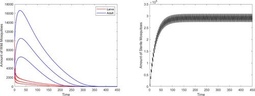2) ) is guaranteed. From Figure 1, we can see that solutions from different initial values all tend to the boundary periodic solution $(0,0,\tilde{g}(t\left)\right)$.

Figure 1. The global stability of the boundary periodic solution of system (2(2) $\left\{\begin{array}{l}\left.\begin{array}{l}\frac{\mathrm{d}J\left(t\right)}{\mathrm{d}t}=\frac{rA\left(t\right)}{A\left(t\right)+g\left(t\right)}A\left(t\right)-\frac{\alpha J\left(t\right)}{\gamma +J\left(t\right)}\\ -(d_0+d_{1}J(t\left)\right)J\left(t\right),\\ \frac{\mathrm{d}A\left(t\right)}{\mathrm{d}t}=\frac{\alpha J\left(t\right)}{\gamma +J\left(t\right)}-{\mu }_{1}A\left(t\right),\\ \frac{\mathrm{d}g\left(t\right)}{\mathrm{d}t}=-{\mu }_{2}g\left(t\right),\end{array}\right\}t\ne kp,k=1,2,\dots ,\\ \left.\begin{array}{l}J\left(t^{+}\right)=J\left(t\right),\\ A\left(t^{+}\right)=A\left(t\right),\\ g\left(t^{+}\right)=g\left(t\right)+\sigma ,\end{array}\right\}t=kp\end{array}\right.$(2) ).

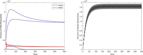
Then reduce the release amount to $\sigma =22,000<{\sigma }^{\ast }\left(3\right)$, we can see that there exists a locally stable positive coexistence periodic solution besides the boundary periodic solution (see Figure 2).

Figure 2. System (2(2) $\left\{\begin{array}{l}\left.\begin{array}{l}\frac{\mathrm{d}J\left(t\right)}{\mathrm{d}t}=\frac{rA\left(t\right)}{A\left(t\right)+g\left(t\right)}A\left(t\right)-\frac{\alpha J\left(t\right)}{\gamma +J\left(t\right)}\\ -(d_0+d_{1}J(t\left)\right)J\left(t\right),\\ \frac{\mathrm{d}A\left(t\right)}{\mathrm{d}t}=\frac{\alpha J\left(t\right)}{\gamma +J\left(t\right)}-{\mu }_{1}A\left(t\right),\\ \frac{\mathrm{d}g\left(t\right)}{\mathrm{d}t}=-{\mu }_{2}g\left(t\right),\end{array}\right\}t\ne kp,k=1,2,\dots ,\\ \left.\begin{array}{l}J\left(t^{+}\right)=J\left(t\right),\\ A\left(t^{+}\right)=A\left(t\right),\\ g\left(t^{+}\right)=g\left(t\right)+\sigma ,\end{array}\right\}t=kp\end{array}\right.$(2) ) has two locally stable periodic solutions with $\sigma =22,000<{\sigma }^{\ast }$: a positive coexistence one and a boundary one.

We next keep the same parameters but fix $\overline{\sigma }=20,000$, then the unique positive solution to equation $\mathcal{H}(\overline{\sigma },p)=R-1$ is $p^{\ast }(20,000)=1.7904$. Then if we extend the release period to $p=3>p^{\ast }(20,000)$, we can see that it also exists a locally stable positive coexistence periodic solution besides the boundary periodic solution (see Figure 3). 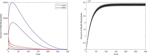While if we shorten the release period to $p=1.5<p^{\ast }(20,000)$, the boundary periodic solution is globally stable (see Figure 4).

Figure 3. System (2(2) $\left\{\begin{array}{l}\left.\begin{array}{l}\frac{\mathrm{d}J\left(t\right)}{\mathrm{d}t}=\frac{rA\left(t\right)}{A\left(t\right)+g\left(t\right)}A\left(t\right)-\frac{\alpha J\left(t\right)}{\gamma +J\left(t\right)}\\ -(d_0+d_{1}J(t\left)\right)J\left(t\right),\\ \frac{\mathrm{d}A\left(t\right)}{\mathrm{d}t}=\frac{\alpha J\left(t\right)}{\gamma +J\left(t\right)}-{\mu }_{1}A\left(t\right),\\ \frac{\mathrm{d}g\left(t\right)}{\mathrm{d}t}=-{\mu }_{2}g\left(t\right),\end{array}\right\}t\ne kp,k=1,2,\dots ,\\ \left.\begin{array}{l}J\left(t^{+}\right)=J\left(t\right),\\ A\left(t^{+}\right)=A\left(t\right),\\ g\left(t^{+}\right)=g\left(t\right)+\sigma ,\end{array}\right\}t=kp\end{array}\right.$(2) ) has two locally stable periodic solutions with $p=3>p^{\ast }$: a positive coexistence one and a boundary one.

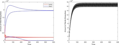
Figure 4. The global stability of the boundary periodic solution of system (2(2) $\left\{\begin{array}{l}\left.\begin{array}{l}\frac{\mathrm{d}J\left(t\right)}{\mathrm{d}t}=\frac{rA\left(t\right)}{A\left(t\right)+g\left(t\right)}A\left(t\right)-\frac{\alpha J\left(t\right)}{\gamma +J\left(t\right)}\\ -(d_0+d_{1}J(t\left)\right)J\left(t\right),\\ \frac{\mathrm{d}A\left(t\right)}{\mathrm{d}t}=\frac{\alpha J\left(t\right)}{\gamma +J\left(t\right)}-{\mu }_{1}A\left(t\right),\\ \frac{\mathrm{d}g\left(t\right)}{\mathrm{d}t}=-{\mu }_{2}g\left(t\right),\end{array}\right\}t\ne kp,k=1,2,\dots ,\\ \left.\begin{array}{l}J\left(t^{+}\right)=J\left(t\right),\\ A\left(t^{+}\right)=A\left(t\right),\\ g\left(t^{+}\right)=g\left(t\right)+\sigma ,\end{array}\right\}t=kp\end{array}\right.$(2) ) with $p=1.5<p^{\ast }$.

3. Optimal control in a limited time

As we have mentioned, the rearing of sterile mosquitoes means huge economic input. Besides, the development of mosquito population has obvious seasonal characteristics and their behaviours have a character of activity peak. Therefore in this section, we consider optimal control problem in a limited time (for example, an activity peak period) and concentrate on reducing wild mosquito population with minimum cost. The main control parameters are release moments and release amount each time.

3.1. Optimization by release timing and release amount

Assume that an amount ${\sigma }_i$ of sterile mosquitoes is released into the environment at moments $t_i\in [0,T]$, $i=1,2,\dots ,N-1$, then a limited-time control system is proposed as follows (11) $\left\{\begin{array}{l}\left.\begin{array}{l}\frac{\mathrm{d}J\left(t\right)}{\mathrm{d}t}=\frac{r{A}^2\left(t\right)}{A\left(t\right)+g\left(t\right)}-\frac{\alpha J\left(t\right)}{\gamma +J\left(t\right)}-(d_0+d_{1}J(t\left)\right)J\left(t\right),\\ \frac{\mathrm{d}A\left(t\right)}{\mathrm{d}t}=\frac{\alpha J\left(t\right)}{\gamma +J\left(t\right)}-{\mu }_{1}A\left(t\right),\\ \frac{\mathrm{d}g\left(t\right)}{\mathrm{d}t}=-{\mu }_{2}g\left(t\right),\end{array}\right\}t\ne t_i,t\in [0,T],\\ \left.\begin{array}{l}J\left(t^{+}\right)=J\left(t\right),A\left(t^{+}\right)=A\left(t\right),\\ g\left(t^{+}\right)=g\left(t\right)+{\sigma }_i,\end{array}\right\}t=t_i,i=1,2,\dots ,N-1\end{array}\right.$(11) with initial conditions (12) $J\left(0\right)=J^0,A\left(0\right)=A^0,g\left(0\right)=g^0.$(12) Here, T>0 is a predefined adjustable constant which stands for the terminal time of control. $t_i,i=1,2,\dots ,N-1$ are the release moments of sterile mosquitoes and satisfy $0=t_0\le t_1\le t_2\le \cdots \le t_{N-1}\le t_N=T$. Let $T_i=t_i-t_{i-1}$ and (13) $0\le T_i^1\le T_i\le T_i^2,i=1,2,\dots ,N,$(13) where $T_i^1$ and $T_i^2$ are given constants which represent the lower and upper bounds of the time interval between the $(i-1)$th and ith release. Besides, we assume that the release amount ${\sigma }_i$ satisfies (14) $0\le {\sigma }_i^1\le {\sigma }_i\le {\sigma }_i^2,i=1,2,\dots ,N-1,$(14) where ${\sigma }_i^1$ and ${\sigma }_i^2$ are also given constants which represent the lower and upper bounds of the amount of the ith release.

Define vectors $\pi =(T_1,T_2,\dots ,T_N{)}^T$ and $\sigma =({\sigma }_1,{\sigma }_2,\dots ,{\sigma }_{N-1}{)}^T$, where $T_i$ and ${\sigma }_i$ satisfy (13(13) $0\le T_i^1\le T_i\le T_i^2,i=1,2,\dots ,N,$(13) ) and (14(14) $0\le {\sigma }_i^1\le {\sigma }_i\le {\sigma }_i^2,i=1,2,\dots ,N-1,$(14) ), respectively. Let ${\mathrm{\Lambda }}_1$ and ${\mathrm{\Lambda }}_2$ denote sets of all $\pi \in R^N,\sigma \in R^{N-1}$ satisfying (13(13) $0\le T_i^1\le T_i\le T_i^2,i=1,2,\dots ,N,$(13) ) and (14(14) $0\le {\sigma }_i^1\le {\sigma }_i\le {\sigma }_i^2,i=1,2,\dots ,N-1,$(14) ), respectively.

Since the functions on the right side of system (11(11) $\left\{\begin{array}{l}\left.\begin{array}{l}\frac{\mathrm{d}J\left(t\right)}{\mathrm{d}t}=\frac{r{A}^2\left(t\right)}{A\left(t\right)+g\left(t\right)}-\frac{\alpha J\left(t\right)}{\gamma +J\left(t\right)}-(d_0+d_{1}J(t\left)\right)J\left(t\right),\\ \frac{\mathrm{d}A\left(t\right)}{\mathrm{d}t}=\frac{\alpha J\left(t\right)}{\gamma +J\left(t\right)}-{\mu }_{1}A\left(t\right),\\ \frac{\mathrm{d}g\left(t\right)}{\mathrm{d}t}=-{\mu }_{2}g\left(t\right),\end{array}\right\}t\ne t_i,t\in [0,T],\\ \left.\begin{array}{l}J\left(t^{+}\right)=J\left(t\right),A\left(t^{+}\right)=A\left(t\right),\\ g\left(t^{+}\right)=g\left(t\right)+{\sigma }_i,\end{array}\right\}t=t_i,i=1,2,\dots ,N-1\end{array}\right.$(11) ) are differentiable, the impulsive system (11(11) $\left\{\begin{array}{l}\left.\begin{array}{l}\frac{\mathrm{d}J\left(t\right)}{\mathrm{d}t}=\frac{r{A}^2\left(t\right)}{A\left(t\right)+g\left(t\right)}-\frac{\alpha J\left(t\right)}{\gamma +J\left(t\right)}-(d_0+d_{1}J(t\left)\right)J\left(t\right),\\ \frac{\mathrm{d}A\left(t\right)}{\mathrm{d}t}=\frac{\alpha J\left(t\right)}{\gamma +J\left(t\right)}-{\mu }_{1}A\left(t\right),\\ \frac{\mathrm{d}g\left(t\right)}{\mathrm{d}t}=-{\mu }_{2}g\left(t\right),\end{array}\right\}t\ne t_i,t\in [0,T],\\ \left.\begin{array}{l}J\left(t^{+}\right)=J\left(t\right),A\left(t^{+}\right)=A\left(t\right),\\ g\left(t^{+}\right)=g\left(t\right)+{\sigma }_i,\end{array}\right\}t=t_i,i=1,2,\dots ,N-1\end{array}\right.$(11) ) with initial condition (12(12) $J\left(0\right)=J^0,A\left(0\right)=A^0,g\left(0\right)=g^0.$(12) ) admits a unique solution $\left(J\right(t),A(t),g(t){)}^T$ corresponding to each pair $(\pi ,\sigma )\in ({\mathrm{\Lambda }}_1,{\mathrm{\Lambda }}_2)$ ([8,9]).

Define a cost function as (15) $\mathcal{J}(\pi ,\sigma )=J\left(T\right)+A\left(T\right)+c_0\sum _{i=1}^{N-1}{\sigma }_i,$(15) where $c_0$ is the cost of sterile mosquitoes per unit.

On the issue of optimal control problem of wild mosquitoes, we can describe it as:

$\left(P1\right)$ For the two-mosquito population system (11(11) $\left\{\begin{array}{l}\left.\begin{array}{l}\frac{\mathrm{d}J\left(t\right)}{\mathrm{d}t}=\frac{r{A}^2\left(t\right)}{A\left(t\right)+g\left(t\right)}-\frac{\alpha J\left(t\right)}{\gamma +J\left(t\right)}-(d_0+d_{1}J(t\left)\right)J\left(t\right),\\ \frac{\mathrm{d}A\left(t\right)}{\mathrm{d}t}=\frac{\alpha J\left(t\right)}{\gamma +J\left(t\right)}-{\mu }_{1}A\left(t\right),\\ \frac{\mathrm{d}g\left(t\right)}{\mathrm{d}t}=-{\mu }_{2}g\left(t\right),\end{array}\right\}t\ne t_i,t\in [0,T],\\ \left.\begin{array}{l}J\left(t^{+}\right)=J\left(t\right),A\left(t^{+}\right)=A\left(t\right),\\ g\left(t^{+}\right)=g\left(t\right)+{\sigma }_i,\end{array}\right\}t=t_i,i=1,2,\dots ,N-1\end{array}\right.$(11) ) with initial condition (12(12) $J\left(0\right)=J^0,A\left(0\right)=A^0,g\left(0\right)=g^0.$(12) ), determine a parameter vector pair $(\pi ,\sigma )\in ({\mathrm{\Lambda }}_1,{\mathrm{\Lambda }}_2)$ to minimize the cost function $\mathcal{J}(\pi ,\sigma )$.

To solve this kind of optimal control problem, there is a technical difficulty for the state of variables $J\left(t\right),A\left(t\right)$ and $g\left(t\right)$ are dependent on uncertain pulse effects (uncertain release timings and uncertain release amounts). To overcome such a difficulty, K. L. Teo [31], X. Y. Liang [25] and Y. Z. Pei [28] and their partners introduced a time rescaling technique, and turned these uncertain pulse time points into fixed ones. In this paper, we apply this method and transform the optimal problem $\left(P1\right)$ into an equivalent optimal parameter selection problem which is described by a series of ODEs with periodic initial conditions. Then we solve the new equivalent problem by applying gradient-based optimization techniques [28].

Let $t=\sum _{j=1}^{i-1}{T}_j+T_{i}s$ for $t\in (\sum _{j=1}^{i-1}{T}_j,\sum _{j=1}^i{T}_j]$, and define (16) $J_i\left(s\right)=J\left(\sum _{j=1}^{i-1}{T}_j+T_{i}s\right),A_i\left(s\right)=A\left(\sum _{j=1}^{i-1}{T}_j+T_{i}s\right),g_i\left(s\right)=g\left(\sum _{j=1}^{i-1}{T}_j+T_{i}s\right).$(16) Then system (11(11) $\left\{\begin{array}{l}\left.\begin{array}{l}\frac{\mathrm{d}J\left(t\right)}{\mathrm{d}t}=\frac{r{A}^2\left(t\right)}{A\left(t\right)+g\left(t\right)}-\frac{\alpha J\left(t\right)}{\gamma +J\left(t\right)}-(d_0+d_{1}J(t\left)\right)J\left(t\right),\\ \frac{\mathrm{d}A\left(t\right)}{\mathrm{d}t}=\frac{\alpha J\left(t\right)}{\gamma +J\left(t\right)}-{\mu }_{1}A\left(t\right),\\ \frac{\mathrm{d}g\left(t\right)}{\mathrm{d}t}=-{\mu }_{2}g\left(t\right),\end{array}\right\}t\ne t_i,t\in [0,T],\\ \left.\begin{array}{l}J\left(t^{+}\right)=J\left(t\right),A\left(t^{+}\right)=A\left(t\right),\\ g\left(t^{+}\right)=g\left(t\right)+{\sigma }_i,\end{array}\right\}t=t_i,i=1,2,\dots ,N-1\end{array}\right.$(11) ) with initial condition (12(12) $J\left(0\right)=J^0,A\left(0\right)=A^0,g\left(0\right)=g^0.$(12) ) is transformed into N subsystems (17) $\left\{\begin{array}{l}\left.\begin{array}{l}\frac{\mathrm{d}{J}_i\left(s\right)}{\mathrm{d}s}=F_1^i\left(s\right)=T_i[\frac{r{A}_i^2\left(s\right)}{A_i\left(s\right)+g_i\left(s\right)}-\frac{\alpha J_i\left(s\right)}{\gamma +J_i\left(s\right)}\\ -(d_0+d_1{J}_i(s\left)\right)J_i\left(s\right)],\\ \frac{\mathrm{d}{A}_i\left(s\right)}{\mathrm{d}s}=F_2^i\left(s\right)=T_i[\frac{\alpha J_i\left(s\right)}{\gamma +J_i\left(s\right)}-{\mu }_1{A}_i(s\left)\right],\\ \frac{\mathrm{d}{g}_i\left(s\right)}{\mathrm{d}s}=F_3^i\left(s\right)=T_i[-{\mu }_2{g}_i(s\left)\right],\end{array}\right\}s\in (0,1],i=1,2,\dots ,N,\\ \left.\begin{array}{l}{J}_i\left(0\right)=J_{i-1}\left(1\right),A_i\left(0\right)=A_{i-1}\left(1\right),g_i\left(0\right)=g_{i-1}\left(1\right)+{\sigma }_i,\end{array}\right\}i=2,3,\dots ,N\end{array}\right.$(17) with (18) $J_1\left(0\right)=J\left(0\right)=J^0,A_1\left(0\right)=A\left(0\right)=A^0,g_1\left(0\right)=g\left(0\right)=g^0.$(18) The cost function (15(15) $\mathcal{J}(\pi ,\sigma )=J\left(T\right)+A\left(T\right)+c_0\sum _{i=1}^{N-1}{\sigma }_i,$(15) ) is transformed into an equivalent new form as (19) ${\mathcal{J}}_1(\pi ,\sigma )=J_N\left(1\right)+A_N\left(1\right)+c_0\sum _{i=1}^{N-1}{\sigma }_i.$(19) Then the optimal control problem $\left(P1\right)$ is converted into

$\left(P2\right)$ For the two-mosquito population system (17(17) $\left\{\begin{array}{l}\left.\begin{array}{l}\frac{\mathrm{d}{J}_i\left(s\right)}{\mathrm{d}s}=F_1^i\left(s\right)=T_i[\frac{r{A}_i^2\left(s\right)}{A_i\left(s\right)+g_i\left(s\right)}-\frac{\alpha J_i\left(s\right)}{\gamma +J_i\left(s\right)}\\ -(d_0+d_1{J}_i(s\left)\right)J_i\left(s\right)],\\ \frac{\mathrm{d}{A}_i\left(s\right)}{\mathrm{d}s}=F_2^i\left(s\right)=T_i[\frac{\alpha J_i\left(s\right)}{\gamma +J_i\left(s\right)}-{\mu }_1{A}_i(s\left)\right],\\ \frac{\mathrm{d}{g}_i\left(s\right)}{\mathrm{d}s}=F_3^i\left(s\right)=T_i[-{\mu }_2{g}_i(s\left)\right],\end{array}\right\}s\in (0,1],i=1,2,\dots ,N,\\ \left.\begin{array}{l}{J}_i\left(0\right)=J_{i-1}\left(1\right),A_i\left(0\right)=A_{i-1}\left(1\right),g_i\left(0\right)=g_{i-1}\left(1\right)+{\sigma }_i,\end{array}\right\}i=2,3,\dots ,N\end{array}\right.$(17) ) with initial condition (18(18) $J_1\left(0\right)=J\left(0\right)=J^0,A_1\left(0\right)=A\left(0\right)=A^0,g_1\left(0\right)=g\left(0\right)=g^0.$(18) ), find a parameter vector pair $(\pi ,\sigma )\in ({\mathrm{\Lambda }}_1,{\mathrm{\Lambda }}_2)$ to minimize the cost function (19(19) ${\mathcal{J}}_1(\pi ,\sigma )=J_N\left(1\right)+A_N\left(1\right)+c_0\sum _{i=1}^{N-1}{\sigma }_i.$(19) ).

Applying the result of Theorem 6.1 in [27], we define corresponding Hamiltonian functions $H_i,i=1,2,\dots ,N,$ (20) $H_i(s,J_i(s),A_i(s),g_i(s),\pi ,\sigma )=\left({\lambda }_1^i\right(s),{\lambda }_2^i(s),{\lambda }_3^i(s\left)\right)\left(F_1^i\right(s),F_2^i(s),F_3^i(s){)}^T,$(20) where ${\lambda }^i\left(s\right)=\left({\lambda }_1^i\right(s),{\lambda }_2^i(s),{\lambda }_3^i(s\left)\right)$ is the corresponding costate which is governed by (21) $\left\{\begin{array}{l}{\dot{\lambda }}_1^i\left(s\right)=-\frac{\mathrm{\partial }H}{\mathrm{\partial }{J}_i}=T_i\left[\right({\lambda }_1^i\left(s\right)-{\lambda }_2^i\left(s\right))\frac{\alpha \gamma }{(\gamma +J_i(s){)}^2}+{\lambda }_1^i(s\left)\right(d_0+2d_1{J}_i\left(s\right)\left)\right],\\ {\dot{\lambda }}_2^i\left(s\right)=-\frac{\mathrm{\partial }H}{\mathrm{\partial }{A}_i}=-T_i\left[{\lambda }_1^i\right(s)\frac{r{A}_i\left(s\right)\left(A_i\right(s)+2g_i(s\left)\right)}{\left(A_i\right(s)+g_i(s){)}^2}-{\mu }_1{\lambda }_2^i(s\left)\right],\\ {\dot{\lambda }}_3^i\left(s\right)=-\frac{\mathrm{\partial }H}{\mathrm{\partial }{g}_i}=T_i\left[{\lambda }_1^i\right(s)\frac{r{A}_i^2\left(s\right)}{\left(A_i\right(s)+g_i(s){)}^2}+{\mu }_2{\lambda }_3^i(s\left)\right]\end{array}\right.$(21) with (22) $\left\{\begin{array}{l}{\lambda }_1^N\left(1\right)=1,{\lambda }_2^N\left(1\right)=1,{\lambda }_3^N\left(1\right)=0,\\ {\lambda }_1^i\left(1\right)={\lambda }_1^{i+1}\left(0\right),{\lambda }_2^i\left(1\right)={\lambda }_2^{i+1}\left(0\right),{\lambda }_3^i\left(1\right)={\lambda }_3^{i+1}\left(0\right),i=2,3,\dots ,N-1.\end{array}\right.$(22) Denote $x_i\left(s\right)=\left(J_i\right(s),A_i(s),g_i(s){)}^T,$then we can easily get from system (17(17) $\left\{\begin{array}{l}\left.\begin{array}{l}\frac{\mathrm{d}{J}_i\left(s\right)}{\mathrm{d}s}=F_1^i\left(s\right)=T_i[\frac{r{A}_i^2\left(s\right)}{A_i\left(s\right)+g_i\left(s\right)}-\frac{\alpha J_i\left(s\right)}{\gamma +J_i\left(s\right)}\\ -(d_0+d_1{J}_i(s\left)\right)J_i\left(s\right)],\\ \frac{\mathrm{d}{A}_i\left(s\right)}{\mathrm{d}s}=F_2^i\left(s\right)=T_i[\frac{\alpha J_i\left(s\right)}{\gamma +J_i\left(s\right)}-{\mu }_1{A}_i(s\left)\right],\\ \frac{\mathrm{d}{g}_i\left(s\right)}{\mathrm{d}s}=F_3^i\left(s\right)=T_i[-{\mu }_2{g}_i(s\left)\right],\end{array}\right\}s\in (0,1],i=1,2,\dots ,N,\\ \left.\begin{array}{l}{J}_i\left(0\right)=J_{i-1}\left(1\right),A_i\left(0\right)=A_{i-1}\left(1\right),g_i\left(0\right)=g_{i-1}\left(1\right)+{\sigma }_i,\end{array}\right\}i=2,3,\dots ,N\end{array}\right.$(17) ) $x_i\left(0\right)=x_{i-1}\left(0\right)+(0,0,{\sigma }_{i-1}{)}^T,i=2,3,\dots ,N.$From Theorems 4.1 and 4.2 in [23], we have

Proposition 3.1

The gradients of the cost functional ${\mathcal{J}}_1$ with respect to σ and π are given by $\frac{\mathrm{\partial }{\mathcal{J}}_1}{\mathrm{\partial }\sigma }=\frac{\mathrm{\partial }(c_0{\displaystyle \sum _{i=1}^{N-1}{\sigma }_i)}}{\mathrm{\partial }\sigma }+\sum _{i=1}^N\left({\lambda }^i\right(0){)}^T\left(\frac{\mathrm{\partial }{x}_i\left(0\right)}{\mathrm{\partial }\sigma }\right)+{\int }_0^1\sum _{i=1}^N\frac{\mathrm{\partial }{H}_i\left(x_i\right(s),\sigma ,\pi ,{\lambda }^i(s\left)\right)}{\mathrm{\partial }\sigma }$and $\frac{\mathrm{\partial }{\mathcal{J}}_1}{\mathrm{\partial }\pi }=\frac{\mathrm{\partial }(c_0{\displaystyle \sum _{i=1}^{N-1}{\sigma }_i)}}{\mathrm{\partial }\pi }+\sum _{i=1}^N\left({\lambda }^i\right(0){)}^T\left(\frac{\mathrm{\partial }{x}_i\left(0\right)}{\mathrm{\partial }\pi }\right)+{\int }_0^1\sum _{i=1}^N\frac{\mathrm{\partial }{H}_i\left(x_i\right(s),\sigma ,\pi ,{\lambda }^i(s\left)\right)}{\mathrm{\partial }\pi },$respectively.

Then by direct calculation, we obtain

Theorem 3.2

The gradients of the cost function ${\mathcal{J}}_1(\pi ,\sigma )$ with respect to the release timing $T_i$ and release amount ${\sigma }_l$ are respectively determined by (23) $\begin{array}{rl}{\mathrm{\nabla }}_{T_i}{\mathcal{J}}_1(\pi ,\sigma )& ={\int }_0^1\sum _j^N\frac{\mathrm{\partial }{H}_j(s,J_j(s),A_j(s),g_j(s),\pi ,\sigma )}{\mathrm{\partial }{T}_i}\mathrm{d}s\\ & ={\int }_0^1\left[{\lambda }_1^i\right(s\left)\right(\frac{r{A}_i^2\left(s\right)}{A_i\left(s\right)+g_i\left(s\right)}-\frac{\alpha J_i\left(s\right)}{\gamma +J_i\left(s\right)}-(d_0+d_1{J}_i(s\left)\right)J_i\left(s\right))\\ & +{\lambda }_2^i\left(s\right)(\frac{\alpha J_i\left(s\right)}{\gamma +J_i\left(s\right)}-{\mu }_1{A}_i(s\left)\right)-{\lambda }_3^i\left(s\right){\mu }_2{g}_i\left(s\right)]\mathrm{d}s\end{array}$(23) for $i=1,2,\dots ,N,$ and (24) $\begin{array}{rl}{\mathrm{\nabla }}_{{\sigma }_l}{\mathcal{J}}_1(\pi ,\sigma )& =c_0+\sum _i^{N-1}\left({\lambda }^{i+1}\right(0{)}^T)\frac{\mathrm{\partial }{\varphi }^i\left(x_i\right(1),{\sigma }_i)}{\mathrm{\partial }{\sigma }_l}\mathrm{d}s\\ & =c_0+\left({\lambda }_1^{l+1}\right(0),{\lambda }_2^{l+1}(0),{\lambda }_3^{l+1}(0\left)\right)(0,0,1{)}^T\\ & =c_0+{\lambda }_3^{l+1}\left(0\right)\end{array}$(24) for $l=1,2,\dots ,N-1$.

3.2. Optimization by release amount for given release period

In this subsection, we consider a situation which is common in the practice. We firstly suppose that sterile mosquitoes are periodically released with a same release amount ${\sigma }_f$ in the limited time $[0,T]$. Assume we plan totally N−1 times of releases, then the release period is $\frac{T}{N}$. That is to say, a fixed amount ${\sigma }_f$ of sterile mosquitoes are released into environment at predefined moments $ip,i=1,2,\dots ,N-1.$ Then the system (11(11) $\left\{\begin{array}{l}\left.\begin{array}{l}\frac{\mathrm{d}J\left(t\right)}{\mathrm{d}t}=\frac{r{A}^2\left(t\right)}{A\left(t\right)+g\left(t\right)}-\frac{\alpha J\left(t\right)}{\gamma +J\left(t\right)}-(d_0+d_{1}J(t\left)\right)J\left(t\right),\\ \frac{\mathrm{d}A\left(t\right)}{\mathrm{d}t}=\frac{\alpha J\left(t\right)}{\gamma +J\left(t\right)}-{\mu }_{1}A\left(t\right),\\ \frac{\mathrm{d}g\left(t\right)}{\mathrm{d}t}=-{\mu }_{2}g\left(t\right),\end{array}\right\}t\ne t_i,t\in [0,T],\\ \left.\begin{array}{l}J\left(t^{+}\right)=J\left(t\right),A\left(t^{+}\right)=A\left(t\right),\\ g\left(t^{+}\right)=g\left(t\right)+{\sigma }_i,\end{array}\right\}t=t_i,i=1,2,\dots ,N-1\end{array}\right.$(11) ) is changed into (25) $\left\{\begin{array}{l}\left.\begin{array}{l}\frac{\mathrm{d}J\left(t\right)}{\mathrm{d}t}=\frac{r{A}^2\left(t\right)}{A\left(t\right)+g\left(t\right)}-\frac{\alpha J\left(t\right)}{\gamma +J\left(t\right)}-(d_0+d_{1}J(t\left)\right)J\left(t\right),\\ \frac{\mathrm{d}A\left(t\right)}{\mathrm{d}t}=\frac{\alpha J\left(t\right)}{\gamma +J\left(t\right)}-{\mu }_{1}A\left(t\right),\\ \frac{\mathrm{d}g\left(t\right)}{\mathrm{d}t}=-{\mu }_{2}g\left(t\right),\end{array}\right\}t\ne ip,t\in [0,T],\\ \left.\begin{array}{l}J\left(i{p}^{+}\right)=J\left(ip\right),A\left(i{p}^{+}\right)=A\left(ip\right),\\ g\left(i{p}^{+}\right)=g\left(ip\right)+{\sigma }_f,\end{array}\right\}t=ip,i=1,2,\dots ,N-1\end{array}\right.$(25) with initial conditions (12(12) $J\left(0\right)=J^0,A\left(0\right)=A^0,g\left(0\right)=g^0.$(12) ).

Besides, we assume that the release amount ${\sigma }_f$ satisfies (26) $0\le {\sigma }_L\le {\sigma }_f\le {\sigma }_U,$(26) where ${\sigma }_L$ and ${\sigma }_U$ are given constants.

For the release period p, we have (27) $Np=T.$(27) Then in this subsection, the cost function of control problem $\left(P1\right)$ is converted into the following form (28) $\overline{\mathcal{J}}\left({\sigma }_f\right)=J\left(T\right)+A\left(T\right)+c_0(N-1){\sigma }_f,$(28) where ${\sigma }_f$ is the only control parameter. That is to say, we need to find a release amount ${\sigma }_f\in [{\sigma }_L,{\sigma }_U]$ such that $\overline{\mathcal{J}}\left({\sigma }_f\right)$ is minimized.

Similarly as we have done above, for $i=1,2,\dots ,N$, let $t=(i-1)p+sp$, then the initial-value problem (25(25) $\left\{\begin{array}{l}\left.\begin{array}{l}\frac{\mathrm{d}J\left(t\right)}{\mathrm{d}t}=\frac{r{A}^2\left(t\right)}{A\left(t\right)+g\left(t\right)}-\frac{\alpha J\left(t\right)}{\gamma +J\left(t\right)}-(d_0+d_{1}J(t\left)\right)J\left(t\right),\\ \frac{\mathrm{d}A\left(t\right)}{\mathrm{d}t}=\frac{\alpha J\left(t\right)}{\gamma +J\left(t\right)}-{\mu }_{1}A\left(t\right),\\ \frac{\mathrm{d}g\left(t\right)}{\mathrm{d}t}=-{\mu }_{2}g\left(t\right),\end{array}\right\}t\ne ip,t\in [0,T],\\ \left.\begin{array}{l}J\left(i{p}^{+}\right)=J\left(ip\right),A\left(i{p}^{+}\right)=A\left(ip\right),\\ g\left(i{p}^{+}\right)=g\left(ip\right)+{\sigma }_f,\end{array}\right\}t=ip,i=1,2,\dots ,N-1\end{array}\right.$(25) ) and (12(12) $J\left(0\right)=J^0,A\left(0\right)=A^0,g\left(0\right)=g^0.$(12) ) is converted into the following N subsystems (29) $\left\{\begin{array}{l}\left.\begin{array}{l}\frac{\mathrm{d}{J}_i\left(s\right)}{\mathrm{d}s}=F_1^i\left(s\right)=p[\frac{r{A}_i^2\left(s\right)}{A_i\left(s\right)+g_i\left(s\right)}-\frac{\alpha J_i\left(s\right)}{\gamma +J_i\left(s\right)}\\ -(d_0+d_1{J}_i(s\left)\right)J_i\left(s\right)],\\ \frac{\mathrm{d}{A}_i\left(s\right)}{\mathrm{d}s}=F_2^i\left(s\right)=p[\frac{\alpha J_i\left(s\right)}{\gamma +J_i\left(s\right)}-{\mu }_1{A}_i(s\left)\right],\\ \frac{\mathrm{d}{g}_i\left(s\right)}{\mathrm{d}s}=F_3^i\left(s\right)=p[-{\mu }_2{g}_i(s\left)\right],\end{array}\right\}s\in (0,1],i=1,2,\dots ,N,\\ \left.\begin{array}{l}{J}_i\left(0\right)=J_{i-1}\left(1\right),A_i\left(0\right)=A_{i-1}\left(1\right),g_i\left(0\right)=g_{i-1}\left(1\right)+{\sigma }_f,\end{array}\right\}i=2,3,\dots ,N\end{array}\right.$(29) with same initial conditions (18(18) $J_1\left(0\right)=J\left(0\right)=J^0,A_1\left(0\right)=A\left(0\right)=A^0,g_1\left(0\right)=g\left(0\right)=g^0.$(18) ).

The cost function (28(28) $\overline{\mathcal{J}}\left({\sigma }_f\right)=J\left(T\right)+A\left(T\right)+c_0(N-1){\sigma }_f,$(28) ) is then equivalently transformed into the following form (30) ${\overline{\mathcal{J}}}_1\left({\sigma }_f\right)=J_N\left(1\right)+A_N\left(1\right)+c_0(N-1){\sigma }_f$(30) and the control problem can be described as: find a ${\sigma }_f\in [{\sigma }_L,{\sigma }_U]$ such that ${\overline{\mathcal{J}}}_1\left({\sigma }_f\right)$ is minimized.

According to the definition of Hamiltonian function in (20(20) $H_i(s,J_i(s),A_i(s),g_i(s),\pi ,\sigma )=\left({\lambda }_1^i\right(s),{\lambda }_2^i(s),{\lambda }_3^i(s\left)\right)\left(F_1^i\right(s),F_2^i(s),F_3^i(s){)}^T,$(20) ), the costate equations (31) $\left\{\begin{array}{l}{\dot{\lambda }}_1^i\left(s\right)=-\frac{\mathrm{\partial }H}{\mathrm{\partial }{J}_i}=p\left[\right({\lambda }_1^i\left(s\right)-{\lambda }_2^i\left(s\right))\frac{\alpha \gamma }{(\gamma +J_i(s){)}^2}+{\lambda }_1^i(s\left)\right(d_0+2d_1{J}_i\left(s\right)\left)\right],\\ {\dot{\lambda }}_2^i\left(s\right)=-\frac{\mathrm{\partial }H}{\mathrm{\partial }{A}_i}=-p\left[{\lambda }_1^i\right(s)\frac{r{A}_i\left(s\right)\left(A_i\right(s)+2g_i(s\left)\right)}{\left(A_i\right(s)+g_i(s){)}^2}-{\mu }_1{\lambda }_2^i(s\left)\right],\\ {\dot{\lambda }}_3^i\left(s\right)=-\frac{\mathrm{\partial }H}{\mathrm{\partial }{g}_i}=p\left[{\lambda }_1^i\right(s)\frac{r{A}_i^2\left(s\right)}{\left(A_i\right(s)+g_i(s){)}^2}+{\mu }_2{\lambda }_3^i(s\left)\right]\end{array}\right.$(31) with boundary conditions (22(22) $\left\{\begin{array}{l}{\lambda }_1^N\left(1\right)=1,{\lambda }_2^N\left(1\right)=1,{\lambda }_3^N\left(1\right)=0,\\ {\lambda }_1^i\left(1\right)={\lambda }_1^{i+1}\left(0\right),{\lambda }_2^i\left(1\right)={\lambda }_2^{i+1}\left(0\right),{\lambda }_3^i\left(1\right)={\lambda }_3^{i+1}\left(0\right),i=2,3,\dots ,N-1.\end{array}\right.$(22) ).

Denote $x_i\left(s\right)=\left(J_i\right(s),A_i(s),g_i(s){)}^T,$and we get from (29(29) $\left\{\begin{array}{l}\left.\begin{array}{l}\frac{\mathrm{d}{J}_i\left(s\right)}{\mathrm{d}s}=F_1^i\left(s\right)=p[\frac{r{A}_i^2\left(s\right)}{A_i\left(s\right)+g_i\left(s\right)}-\frac{\alpha J_i\left(s\right)}{\gamma +J_i\left(s\right)}\\ -(d_0+d_1{J}_i(s\left)\right)J_i\left(s\right)],\\ \frac{\mathrm{d}{A}_i\left(s\right)}{\mathrm{d}s}=F_2^i\left(s\right)=p[\frac{\alpha J_i\left(s\right)}{\gamma +J_i\left(s\right)}-{\mu }_1{A}_i(s\left)\right],\\ \frac{\mathrm{d}{g}_i\left(s\right)}{\mathrm{d}s}=F_3^i\left(s\right)=p[-{\mu }_2{g}_i(s\left)\right],\end{array}\right\}s\in (0,1],i=1,2,\dots ,N,\\ \left.\begin{array}{l}{J}_i\left(0\right)=J_{i-1}\left(1\right),A_i\left(0\right)=A_{i-1}\left(1\right),g_i\left(0\right)=g_{i-1}\left(1\right)+{\sigma }_f,\end{array}\right\}i=2,3,\dots ,N\end{array}\right.$(29) ) $x_i\left(0\right)=x_{i-1}\left(0\right)+(0,0,{\sigma }_f{)}^T,i=2,3,\dots ,N.$Then by the same method, we get

Theorem 3.3

The gradient of ${\overline{\mathcal{J}}}_1\left({\sigma }_f\right)$ with respect to the release amount ${\sigma }_f$ is (32) $\mathrm{\nabla }{\overline{\mathcal{J}}}_1\left({\sigma }_f\right)=c_0(N-1)+\sum _i^{N-1}{\lambda }_3^{i+1}\left(0\right).$(32)

3.3. Optimization by release timing for given release amount

In this subsection, we consider another situation which is also common in the practice. Assume that sterile mosquitoes are released at irregular moments $0\le t_1\le t_2\le \cdots \le t_{N-1}\le T$ with a same release amount ${\sigma }_f$. Here, the release amount ${\sigma }_f$ and release timing $t_1,t_2,\dots ,t_{N-1}$ are all decision variables. Then the system (11(11) $\left\{\begin{array}{l}\left.\begin{array}{l}\frac{\mathrm{d}J\left(t\right)}{\mathrm{d}t}=\frac{r{A}^2\left(t\right)}{A\left(t\right)+g\left(t\right)}-\frac{\alpha J\left(t\right)}{\gamma +J\left(t\right)}-(d_0+d_{1}J(t\left)\right)J\left(t\right),\\ \frac{\mathrm{d}A\left(t\right)}{\mathrm{d}t}=\frac{\alpha J\left(t\right)}{\gamma +J\left(t\right)}-{\mu }_{1}A\left(t\right),\\ \frac{\mathrm{d}g\left(t\right)}{\mathrm{d}t}=-{\mu }_{2}g\left(t\right),\end{array}\right\}t\ne t_i,t\in [0,T],\\ \left.\begin{array}{l}J\left(t^{+}\right)=J\left(t\right),A\left(t^{+}\right)=A\left(t\right),\\ g\left(t^{+}\right)=g\left(t\right)+{\sigma }_i,\end{array}\right\}t=t_i,i=1,2,\dots ,N-1\end{array}\right.$(11) ) is rewritten as (33) $\left\{\begin{array}{l}\left.\begin{array}{l}\frac{\mathrm{d}J\left(t\right)}{\mathrm{d}t}=\frac{r{A}^2\left(t\right)}{A\left(t\right)+g\left(t\right)}-\frac{\alpha J\left(t\right)}{\gamma +J\left(t\right)}-(d_0+d_{1}J(t\left)\right)J\left(t\right),\\ \frac{\mathrm{d}A\left(t\right)}{\mathrm{d}t}=\frac{\alpha J\left(t\right)}{\gamma +J\left(t\right)}-{\mu }_{1}A\left(t\right),\\ \frac{\mathrm{d}g\left(t\right)}{\mathrm{d}t}=-{\mu }_{2}g\left(t\right),\end{array}\right\}t\ne t_i,t\in [0,T],\\ \left.\begin{array}{l}J\left(t_i^{+}\right)=J\left(t_i\right),A\left(t_i^{+}\right)=A\left(t_i\right),\\ g\left(t_i^{+}\right)=g\left(t_i\right)+{\sigma }_f,\end{array}\right\}t=t_i,i=1,2,\dots ,N-1\end{array}\right.$(33) with initial conditions (12(12) $J\left(0\right)=J^0,A\left(0\right)=A^0,g\left(0\right)=g^0.$(12) ). Here, $t_i,i=1,2,\dots ,N$ and ${\sigma }_f$ satisfy conditions (13(13) $0\le T_i^1\le T_i\le T_i^2,i=1,2,\dots ,N,$(13) ) and (26(26) $0\le {\sigma }_L\le {\sigma }_f\le {\sigma }_U,$(26) ), respectively.

The cost function of control problem $\left(P1\right)$ is changed into the following form (34) $\stackrel{\mathcal{ˆ}}{\mathcal{J}}(\pi ,{\sigma }_f)=J\left(T\right)+A\left(T\right)+c_0(N-1){\sigma }_f,$(34) where $\pi =(T_1,T_2,\dots \cdots ,T_N{)}^T,T_i=t_i-t_{i-1}$.

Let $t=\sum _{j=1}^{i-1}{T}_j+T_{i}s$ for $i=1,2,\dots ,N$, and the system (33(33) $\left\{\begin{array}{l}\left.\begin{array}{l}\frac{\mathrm{d}J\left(t\right)}{\mathrm{d}t}=\frac{r{A}^2\left(t\right)}{A\left(t\right)+g\left(t\right)}-\frac{\alpha J\left(t\right)}{\gamma +J\left(t\right)}-(d_0+d_{1}J(t\left)\right)J\left(t\right),\\ \frac{\mathrm{d}A\left(t\right)}{\mathrm{d}t}=\frac{\alpha J\left(t\right)}{\gamma +J\left(t\right)}-{\mu }_{1}A\left(t\right),\\ \frac{\mathrm{d}g\left(t\right)}{\mathrm{d}t}=-{\mu }_{2}g\left(t\right),\end{array}\right\}t\ne t_i,t\in [0,T],\\ \left.\begin{array}{l}J\left(t_i^{+}\right)=J\left(t_i\right),A\left(t_i^{+}\right)=A\left(t_i\right),\\ g\left(t_i^{+}\right)=g\left(t_i\right)+{\sigma }_f,\end{array}\right\}t=t_i,i=1,2,\dots ,N-1\end{array}\right.$(33) ) is reduced to (35) $\left\{\begin{array}{l}\left.\begin{array}{l}\frac{\mathrm{d}{J}_i\left(s\right)}{\mathrm{d}s}=F_1^i\left(s\right)=T_i[\frac{r{A}_i^2\left(s\right)}{A_i\left(s\right)+g_i\left(s\right)}-\frac{\alpha J_i\left(s\right)}{\gamma +J_i\left(s\right)}\\ -(d_0+d_1{J}_i(s\left)\right)J_i\left(s\right)],\\ \frac{\mathrm{d}{A}_i\left(s\right)}{\mathrm{d}s}=F_2^i\left(s\right)=T_i[\frac{\alpha J_i\left(s\right)}{\gamma +J_i\left(s\right)}-{\mu }_1{A}_i(s\left)\right],\\ \frac{\mathrm{d}{g}_i\left(s\right)}{\mathrm{d}s}=F_3^i\left(s\right)=T_i[-{\mu }_2{g}_i(s\left)\right],\end{array}\right\}s\in (0,1],i=1,2,\dots ,N,\\ \left.\begin{array}{l}{J}_i\left(0\right)=J_{i-1}\left(1\right),A_i\left(0\right)=A_{i-1}\left(1\right),g_i\left(0\right)=g_{i-1}\left(1\right)+{\sigma }_f,\end{array}\right\}i=2,3,\dots ,N\end{array}\right.$(35) with initial conditions (18(18) $J_1\left(0\right)=J\left(0\right)=J^0,A_1\left(0\right)=A\left(0\right)=A^0,g_1\left(0\right)=g\left(0\right)=g^0.$(18) ).

Similarly, cost function (34(34) $\stackrel{\mathcal{ˆ}}{\mathcal{J}}(\pi ,{\sigma }_f)=J\left(T\right)+A\left(T\right)+c_0(N-1){\sigma }_f,$(34) ) is converted into (36) ${\stackrel{\mathcal{ˆ}}{\mathcal{J}}}_1(\pi ,{\sigma }_f)=J_N\left(1\right)+A_N\left(1\right)+c_0(N-1){\sigma }_f.$(36) For the Hamiltonian function $H_i(s,J_i(s),A_i(s),g_i(s),\pi ,{\sigma }_f)$ defined in (20(20) $H_i(s,J_i(s),A_i(s),g_i(s),\pi ,\sigma )=\left({\lambda }_1^i\right(s),{\lambda }_2^i(s),{\lambda }_3^i(s\left)\right)\left(F_1^i\right(s),F_2^i(s),F_3^i(s){)}^T,$(20) ), we get the same corresponding costate Equation (21(21) $\left\{\begin{array}{l}{\dot{\lambda }}_1^i\left(s\right)=-\frac{\mathrm{\partial }H}{\mathrm{\partial }{J}_i}=T_i\left[\right({\lambda }_1^i\left(s\right)-{\lambda }_2^i\left(s\right))\frac{\alpha \gamma }{(\gamma +J_i(s){)}^2}+{\lambda }_1^i(s\left)\right(d_0+2d_1{J}_i\left(s\right)\left)\right],\\ {\dot{\lambda }}_2^i\left(s\right)=-\frac{\mathrm{\partial }H}{\mathrm{\partial }{A}_i}=-T_i\left[{\lambda }_1^i\right(s)\frac{r{A}_i\left(s\right)\left(A_i\right(s)+2g_i(s\left)\right)}{\left(A_i\right(s)+g_i(s){)}^2}-{\mu }_1{\lambda }_2^i(s\left)\right],\\ {\dot{\lambda }}_3^i\left(s\right)=-\frac{\mathrm{\partial }H}{\mathrm{\partial }{g}_i}=T_i\left[{\lambda }_1^i\right(s)\frac{r{A}_i^2\left(s\right)}{\left(A_i\right(s)+g_i(s){)}^2}+{\mu }_2{\lambda }_3^i(s\left)\right]\end{array}\right.$(21) ) with boundary conditions (22(22) $\left\{\begin{array}{l}{\lambda }_1^N\left(1\right)=1,{\lambda }_2^N\left(1\right)=1,{\lambda }_3^N\left(1\right)=0,\\ {\lambda }_1^i\left(1\right)={\lambda }_1^{i+1}\left(0\right),{\lambda }_2^i\left(1\right)={\lambda }_2^{i+1}\left(0\right),{\lambda }_3^i\left(1\right)={\lambda }_3^{i+1}\left(0\right),i=2,3,\dots ,N-1.\end{array}\right.$(22) ).

Then, we have

Theorem 3.4

The gradients of ${\stackrel{\mathcal{ˆ}}{\mathcal{J}}}_1(\pi ,{\sigma }_f)$ with respect to the release timing $T_k$ and release amount ${\sigma }_f$ are (37) ${\mathrm{\nabla }}_{T_k}{\stackrel{\mathcal{ˆ}}{\mathcal{J}}}_1(\pi ,{\sigma }_f)={\mathrm{\nabla }}_{T_k}{\mathcal{J}}_1(\pi ,\sigma ),k=1,2,\dots ,N$(37) and (38) ${\mathrm{\nabla }}_{{\sigma }_f}{\stackrel{\mathcal{ˆ}}{\mathcal{J}}}_1(\pi ,{\sigma }_f)=c_0(N-1)+\sum _i^{N-1}{\lambda }_3^{i+1}\left(0\right).$(38) Here ${\mathrm{\nabla }}_{T_k}{\mathcal{J}}_1(\pi ,\sigma )$ is defined in (23(23) $\begin{array}{rl}{\mathrm{\nabla }}_{T_i}{\mathcal{J}}_1(\pi ,\sigma )& ={\int }_0^1\sum _j^N\frac{\mathrm{\partial }{H}_j(s,J_j(s),A_j(s),g_j(s),\pi ,\sigma )}{\mathrm{\partial }{T}_i}\mathrm{d}s\\ & ={\int }_0^1\left[{\lambda }_1^i\right(s\left)\right(\frac{r{A}_i^2\left(s\right)}{A_i\left(s\right)+g_i\left(s\right)}-\frac{\alpha J_i\left(s\right)}{\gamma +J_i\left(s\right)}-(d_0+d_1{J}_i(s\left)\right)J_i\left(s\right))\\ & +{\lambda }_2^i\left(s\right)(\frac{\alpha J_i\left(s\right)}{\gamma +J_i\left(s\right)}-{\mu }_1{A}_i(s\left)\right)-{\lambda }_3^i\left(s\right){\mu }_2{g}_i\left(s\right)]\mathrm{d}s\end{array}$(23) ).

4. Numerical simulations for the optimal control

In this section, a series of numerical simulations for systems (11(11) $\left\{\begin{array}{l}\left.\begin{array}{l}\frac{\mathrm{d}J\left(t\right)}{\mathrm{d}t}=\frac{r{A}^2\left(t\right)}{A\left(t\right)+g\left(t\right)}-\frac{\alpha J\left(t\right)}{\gamma +J\left(t\right)}-(d_0+d_{1}J(t\left)\right)J\left(t\right),\\ \frac{\mathrm{d}A\left(t\right)}{\mathrm{d}t}=\frac{\alpha J\left(t\right)}{\gamma +J\left(t\right)}-{\mu }_{1}A\left(t\right),\\ \frac{\mathrm{d}g\left(t\right)}{\mathrm{d}t}=-{\mu }_{2}g\left(t\right),\end{array}\right\}t\ne t_i,t\in [0,T],\\ \left.\begin{array}{l}J\left(t^{+}\right)=J\left(t\right),A\left(t^{+}\right)=A\left(t\right),\\ g\left(t^{+}\right)=g\left(t\right)+{\sigma }_i,\end{array}\right\}t=t_i,i=1,2,\dots ,N-1\end{array}\right.$(11) ), (25(25) $\left\{\begin{array}{l}\left.\begin{array}{l}\frac{\mathrm{d}J\left(t\right)}{\mathrm{d}t}=\frac{r{A}^2\left(t\right)}{A\left(t\right)+g\left(t\right)}-\frac{\alpha J\left(t\right)}{\gamma +J\left(t\right)}-(d_0+d_{1}J(t\left)\right)J\left(t\right),\\ \frac{\mathrm{d}A\left(t\right)}{\mathrm{d}t}=\frac{\alpha J\left(t\right)}{\gamma +J\left(t\right)}-{\mu }_{1}A\left(t\right),\\ \frac{\mathrm{d}g\left(t\right)}{\mathrm{d}t}=-{\mu }_{2}g\left(t\right),\end{array}\right\}t\ne ip,t\in [0,T],\\ \left.\begin{array}{l}J\left(i{p}^{+}\right)=J\left(ip\right),A\left(i{p}^{+}\right)=A\left(ip\right),\\ g\left(i{p}^{+}\right)=g\left(ip\right)+{\sigma }_f,\end{array}\right\}t=ip,i=1,2,\dots ,N-1\end{array}\right.$(25) ) and (33(33) $\left\{\begin{array}{l}\left.\begin{array}{l}\frac{\mathrm{d}J\left(t\right)}{\mathrm{d}t}=\frac{r{A}^2\left(t\right)}{A\left(t\right)+g\left(t\right)}-\frac{\alpha J\left(t\right)}{\gamma +J\left(t\right)}-(d_0+d_{1}J(t\left)\right)J\left(t\right),\\ \frac{\mathrm{d}A\left(t\right)}{\mathrm{d}t}=\frac{\alpha J\left(t\right)}{\gamma +J\left(t\right)}-{\mu }_{1}A\left(t\right),\\ \frac{\mathrm{d}g\left(t\right)}{\mathrm{d}t}=-{\mu }_{2}g\left(t\right),\end{array}\right\}t\ne t_i,t\in [0,T],\\ \left.\begin{array}{l}J\left(t_i^{+}\right)=J\left(t_i\right),A\left(t_i^{+}\right)=A\left(t_i\right),\\ g\left(t_i^{+}\right)=g\left(t_i\right)+{\sigma }_f,\end{array}\right\}t=t_i,i=1,2,\dots ,N-1\end{array}\right.$(33) ) are performed, which not only confirm the results we obtained in Section 3, but also complement them with specific features.

To begin with, let us present the detailed steps for the computation of the cost function and its gradients with respect to the control parameters [28], [23]. We will focus on the case in Section 3.1.

1. We first solve directly the dynamical system (17(17) $\left\{\begin{array}{l}\left.\begin{array}{l}\frac{\mathrm{d}{J}_i\left(s\right)}{\mathrm{d}s}=F_1^i\left(s\right)=T_i[\frac{r{A}_i^2\left(s\right)}{A_i\left(s\right)+g_i\left(s\right)}-\frac{\alpha J_i\left(s\right)}{\gamma +J_i\left(s\right)}\\ -(d_0+d_1{J}_i(s\left)\right)J_i\left(s\right)],\\ \frac{\mathrm{d}{A}_i\left(s\right)}{\mathrm{d}s}=F_2^i\left(s\right)=T_i[\frac{\alpha J_i\left(s\right)}{\gamma +J_i\left(s\right)}-{\mu }_1{A}_i(s\left)\right],\\ \frac{\mathrm{d}{g}_i\left(s\right)}{\mathrm{d}s}=F_3^i\left(s\right)=T_i[-{\mu }_2{g}_i(s\left)\right],\end{array}\right\}s\in (0,1],i=1,2,\dots ,N,\\ \left.\begin{array}{l}{J}_i\left(0\right)=J_{i-1}\left(1\right),A_i\left(0\right)=A_{i-1}\left(1\right),g_i\left(0\right)=g_{i-1}\left(1\right)+{\sigma }_i,\end{array}\right\}i=2,3,\dots ,N\end{array}\right.$(17) ) with initial conditions (18(18) $J_1\left(0\right)=J\left(0\right)=J^0,A_1\left(0\right)=A\left(0\right)=A^0,g_1\left(0\right)=g\left(0\right)=g^0.$(18) ) for $i=1,2,\dots ,N$ to obtain $J_i\left(s\right),A_i\left(s\right),g_i\left(s\right),s\in [0,1]$.

2. Applying $J_i\left(s\right),A_i\left(s\right),g_i\left(s\right)$ that have been obtained in last

   boundary conditions (22(22) $\left\{\begin{array}{l}{\lambda }_1^N\left(1\right)=1,{\lambda }_2^N\left(1\right)=1,{\lambda }_3^N\left(1\right)=0,\\ {\lambda }_1^i\left(1\right)={\lambda }_1^{i+1}\left(0\right),{\lambda }_2^i\left(1\right)={\lambda }_2^{i+1}\left(0\right),{\lambda }_3^i\left(1\right)={\lambda }_3^{i+1}\left(0\right),i=2,3,\dots ,N-1.\end{array}\right.$(22) ) and get ${\lambda }_1^i\left(s\right),{\lambda }_2^i\left(s\right)$ and ${\lambda }_3^i\left(s\right)$ for $i=1,2,\dots ,N$.

3. According to (19(19) ${\mathcal{J}}_1(\pi ,\sigma )=J_N\left(1\right)+A_N\left(1\right)+c_0\sum _{i=1}^{N-1}{\sigma }_i.$(19) ), we calculate the cost function ${\mathcal{J}}_1(\pi ,\sigma )$ by using $J_i\left(s\right)$, $A_i\left(s\right)$ and $g_i\left(s\right)$.

4. Applying $J_i\left(s\right),A_i\left(s\right),g_i\left(s\right),{\lambda }_1^i\left(s\right),{\lambda }_2^i\left(s\right)$ and ${\lambda }_3^i\left(s\right)$, we calculate ${\mathrm{\nabla }}_{T_i}{\mathcal{J}}_1(\pi ,\sigma )$ for $i=1,2,\dots ,N$ and ${\mathrm{\nabla }}_{{\sigma }_l}{\mathcal{J}}_1(\pi ,\sigma )$ for $l=1,2,\dots ,N-1$.

Still choose the parameters given in Table 1, and if no sterile mosquito is released into the environment, the larvae and the adults of wild mosquito population will remain stable at certain level in the long run. In our numerical experiments, time is measured in days and we take 15 days as the total control time, that is, T = 15. These 15 days will be divided into N = 5 parts, and sterile mosquitoes will be released N−1 = 4 times in different forms. Suppose that the cost of one sterile mosquito production and its release is 0.02, then we have $c_0=0.02$.

In the following, we will study three different optimal strategies in impulsive control by numerical simulations. Surely there is no guarantee that the optimal solution we find numerically is unique, so we just present some optimal ones with special initial release periods and amounts by the above steps.

Besides, different constraint intervals for control parameters will lead to different optimal solutions. In some field trials, sterile mosquitoes are always released at a specific frequency and quantity. For example in previous study [40], the researchers undertook an open-release field trial in two islands in the city of Guangzhou, a city with the highest dengue transmission rate in China, and sterile mosquitoes were released two or three times a week with 70,000–1,00,000 each time. Hence, in our study we also designed the upper and lower bounds of the release interval and quantity to describe these practical operation characteristics.

Example 4.1

Optimal release amount for fixed release period

For a fixed release period p = 3, starting with a initial release amount ${\sigma }_f=30,000$, we can obtain that the cost value ${\mathcal{J}}_0=2.1556\times {10}^4$ and the total wild mosquito population $J\left(T\right)+A\left(T\right)=1.9156\times {10}^4$ at T = 15.

With the constraint condition $0\le {\sigma }_f\le 1,00,000$, we solve the optimal problem through the above algorithm by using Matlab program and get an optimal release amount ${\sigma }_f^{\ast }=5.7350\times {10}^4$ and the corresponding cost value ${\mathcal{J}}^{\ast }=2.0550\times {10}^4$, while the total wild mosquito population at the terminal time is $J^{\ast }\left(T\right)+A^{\ast }\left(T\right)=1.5962\times {10}^4$. We compare this optimal control with non-control and simple impulsive control in Figure 5(a), and find that it has an obvious superiority. In most time of the control process, the total wild mosquito population (the larvae and the adults) of the optimal one is much less than that of the other two methods.

Figure 5. Release amount control: (a) Comparisons of total wild mosquitoes population under different biological controls; (b) Impact of the intensity of each release on the objective function and wild mosquito population at time T.

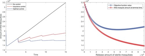
Besides, we exploit the impact of the intensity of each release on the objective function and wild mosquito population at terminal time T in Figure 5(b). When the release amount varies in the interval $0\le {\sigma }_f\le 1,00,000$, there is a minimum value which verifies the optimum value we have obtained. In addition, we find that with the increase of the release amount, the wild mosquito population at the terminal time T continues decreasing. However, the wild mosquito cannot be eliminated even if the release amount reaches the upper constrained boundary and the cost value is really quite high.

Example 4.2

Optimal release timing for same release amount

Start with a initial release amount of sterile mosquitoes ${\sigma }_f=30,000$ and initial release intervals $T_1=T_2=\cdots =T_5=3$. To determine optimal time intervals $T_i$ and optimal releasing amount ${\sigma }_f$ that can guarantee the minimal cost function $\mathcal{J}$, we give constraint conditions (39) $0\le T_i\le 10,i=1,2,\dots ,5,\sum _1^5{T}_i=15$(39) and $0\le {\sigma }_f\le 1,00,000$.

Then we solve the optimal problem and obtain a set of optimal release intervals (40) $T_1^{\ast }=0.0405,T_2^{\ast }=0.2126,T_3^{\ast }=0.2126,T_4^{\ast }=4.5363,T_5^{\ast }=9.9980$(40) and an optimal release amount (41) ${\sigma }_f^{\ast }=5.5040\times {10}^4.$(41) Such a control strategy is described by Figure 6(b). Besides, the minimum cost value we gained is ${\mathcal{J}}^{\ast }=1.6510\times {10}^4$ while the total wild mosquito population at the terminal time is $J^{\ast }\left(T\right)+A^{\ast }\left(T\right)=1.2107\times {10}^4$.

Figure 6. Release timing control: (a) Comparisons of total wild mosquitoes population under different biological controls; (b) Release strategy of the mixed optimal control; (c) Impact of the intensity of each release on the optimal cost value and wild mosquito population at time T; (d) Errors of the cost function $\mathcal{J}$ in each iteration for optimal release timing control.

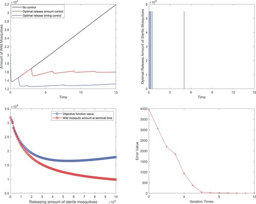
We also compare the optimal release timing control with non-control and optimal release amount control in Figure 6(a), and find that with much less sterile mosquitoes releasing, the former one has obvious advantages in the realization of control objective. It can also make the wild mosquito population in a much lower level for a long time. In addition, the relative errors of the cost value $\mathcal{J}$ with respect to the optimal one ${\mathcal{J}}^{\ast }$ at each iteration step are plotted in Figure 6(d), and the convergence of our algorithm is validated by both Figure 6(d) and Table 2.

Table 2. Values of the cost function in the iteration process for optimal release timing control.

Number of iterations	0	3	6	9	12
$\mathcal{J}(\times {10}^4)$	2.1556	1.9443	1.7638	1.6799	1.6510

Furthermore, for each ${\sigma }_f\in [0,100,000]$, we determine the corresponding optimal time intervals with the restriction (39(39) $0\le T_i\le 10,i=1,2,\dots ,5,\sum _1^5{T}_i=15$(39) ) and then calculate the value of cost function and the amount of wild mosquitoes at the terminal time. The results are displayed in Figure 6(c). When the release amount varies in the interval $0\le {\sigma }_f\le 1,00,000$, there is a minimum value which also verifies the optimum values we have obtained. Similarly, with the increase of the release amount, the wild mosquito population also keeps going down but it cannot be eliminated no matter how many sterile mosquitoes are released each time.

Example 4.3

Optimal release timing and release amounts

We still take the initial release intervals $T_1=T_2=\cdots =T_5=3$ and choose initial release amounts ${\sigma }_1={\sigma }_2=\cdots ={\sigma }_4=30,000$ subjected to constraint conditions (39(39) $0\le T_i\le 10,i=1,2,\dots ,5,\sum _1^5{T}_i=15$(39) ) and $0\le {\sigma }_i\le 1,00,000,i=1,2,3,4$. We solve the optimal problem and obtain a set of optimal release amounts (42) ${\sigma }_1^{\ast }=9.9940\times {10}^4,{\sigma }_2^{\ast }=9.9940\times {10}^4,{\sigma }_3^{\ast }=0.8640\times {10}^4,{\sigma }_4^{\ast }=0.8640\times {10}^4$(42) and a set of optimal release intervals (43) $T_1^{\ast }=0.0162,T_2^{\ast }=0.1025,T_3^{\ast }=0.2025,T_4^{\ast }=4.6789,T_5^{\ast }=\mathrm{9.9999.}$(43) This control strategy is described by Figure 7(c). Besides, the minimum cost value is ${\mathcal{J}}^{\ast }=1.5965\times {10}^4$ while the total wild mosquito population at terminal time is $J^{\ast }\left(T\right)+A^{\ast }\left(T\right)=1.1965\times {10}^4$.The trajectories of total wild mosquitoes (the larvae and the adults of wild mosquito population) under four types of control modes are shown in Figure 7(a) and we can see that mixed optimal control has the most obvious advantages, then followed by optimal timing control and optimal release amount control. While Figure 7(b) tells us that the mixed optimal control releases the least sterile mosquitoes in the whole control process, while the optimal amount control releases the most sterile mosquitoes. In addition, the relative errors of the cost value $\mathcal{J}$ with respect to the optimal one ${\mathcal{J}}^{\ast }$ at each iteration step are described in Figure 7(d), and the convergence of our algorithm is verified by both Figure 7(d) and Table 3.

Figure 7. Mixed control: (a) Comparisons of total wild mosquitoes population under different biological controls; (b) Comparisons of total release amounts of sterile mosquitoes for three optimal control methods; (c) Release strategy of the mixed optimal control; (d) Errors of the cost function $\mathcal{J}$ in each iteration for mixed optimal control.

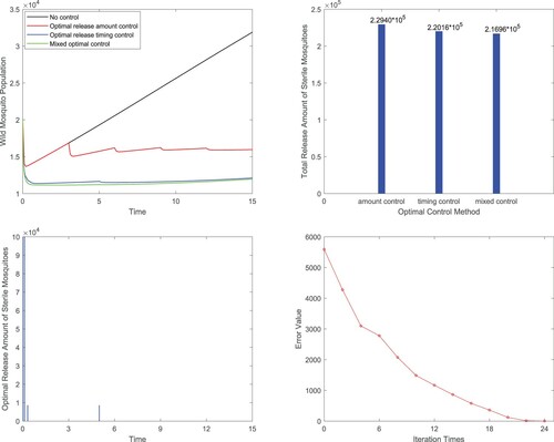
Finally, three optimal release strategies are compared with each other (refer to Table 4). We can see that for optimal control, the optimal selection of release timing is more important than the optimal selection of release amount. However, mixed optimal control is the best option. Combining with Figure 7(b), we know that although the optimal amount control releases the most sterile mosquitoes in the whole control process, but the control effect is the worst.

Table 3. Values of the cost function in the iteration process for optimal mixed control.

Number of iterations	0	6	12	18	24
$\mathcal{J}(\times {10}^4)$	2.1556	1.8746	1.7132	1.6324	1.5965

Table 4. Comparison of different release strategies.

	Optimal control parameters	${\mathcal{J}}^{\ast }$	$J^{\ast }\left(T\right)+A^{\ast }\left(T\right)$
Release amount control	${\sigma }_f^{\ast }=57350$	20,550	15,962
	$T_1^{\ast }=0.0405$, $T_2^{\ast }=0.2126$,
Release timing control	$T_3^{\ast }=0.2126$, $T_4^{\ast }=4.5363$,	16,510	12,107
	$T_5^{\ast }=9.9980$, ${\sigma }_f^{\ast }=55,040$
	$T_1^{\ast }=0.0162$, $T_2^{\ast }=0.1025$,
	$T_3^{\ast }=0.2025$, $T_4^{\ast }=4.6789$,
Mixed control	$T_5^{\ast }=9.9999$, ${\sigma }_1^{\ast }=99,940$	15,965	11,965
	${\sigma }_2^{\ast }=99,940$, ${\sigma }_3^{\ast }=8640$
	${\sigma }_4^{\ast }=8640$

5. Conclusion

As a method of biological control, SIT has been successfully used to disturb the development of the wild mosquito population in an environment. A large number of mathematical models have been proposed to investigate the release strategies of sterile mosquitoes for the population control of wild ones. However, most of these models focus on continuous release mode which is not consistent with the actual situation. In this paper, we propose impulsive dynamical systems for the interaction between two mosquito populations incorporating impulsive releases of sterile ones, and concentrate on the release strategies for the long-term and limited- time control of wild mosquitoes.

We first study the long-term control system with regular impulsive sterile mosquito releases. The dynamical behaviours, such as the existence, uniqueness and globally stability of the boundary periodic solution (wild mosquito extinction) are qualitatively analysed. In addition, thresholds of the release amount and release period are gained which can guarantee that the wild mosquito population is eliminated in the long run. Comparing the results we obtained with the study of periodic release strategy under open-loop control in [10], we find consistency although they use different modelling approaches.

Then for the limited-time control model, three different optimal strategies in impulsive control (release amount control, release timing control and mixed control) aiming at minimizing the amount of wild mosquitoes at the terminal time and reducing the economic cost are investigated. To overcome the technical difficulty of the optimal control problem which is caused by uncertain pulse effects, a time rescaling technique and an optimization algorithm based on gradient are applied. Using gradient formulas we have gained, optimal impulsive release timings and release amounts of sterile mosquitoes are obtained by numerical simulations. In addition, our simulations indicate that for optimal control, the optimal selection of release timing is more important than the optimal selection of release amount, while mixed optimal control has the best comprehensive effect.

In the limited-time control, we notice that whether wild mosquitoes can be better controlled depends on whether sterile mosquitoes are released earlier and more vigorously. Thus during the early stage of the control time, the evolution of wild mosquitoes is disturbed violently with respect to the natural one and the number of wild mosquitoes in the environment falls rapidly. This conclusion is very similar to that of long-term control of wild mosquitoes.

Acknowledgments

We are grateful to Professor Jia Li whose contribution to this work was of great significance.

Disclosure statement

No potential conflict of interest was reported by the author(s).

Additional information

Funding

Mingzhan Huang was partially supported by Foundation for Distinguished Young Talents in Higher Education of Henan [grant number 2019GGJS157], Foundation of Henan Educational Committee under Contract [grant number 21A110022], Program for Science & Technology Innovation Talents in Universities of Henan Province [grant number 21HASTIT026], Scientific and Technological Key Projects of Henan Province [grant number 212102110025] and Nanhu Scholars Program for Young Scholars of XYNU. Lei You, Shouzong Liu and Xinyu Song were partially supported by the National Natural Science Foundation of China [grant number 12071407], [grant number 11901502], [grant number 31872704], [grant number 11871415] and Nanhu Scholars Program of XYNU.

Appendix

Similar to the discussion in [24]. Since $A^{\ast }=\frac{\alpha J^{\ast }}{{\mu }_1(\gamma +J^{\ast })},\frac{r{A}^{\ast }}{A^{\ast }+g_{\mathrm{c}\mathrm{o}\mathrm{n}\mathrm{s}\mathrm{t}}}{A}^{\ast }=\frac{\alpha J^{\ast }}{\gamma +J^{\ast }}+(d_0+d_1{J}^{\ast })J^{\ast },$we can easily get $\frac{r\alpha J^{\ast }}{{\mu }_1\gamma g_{\mathrm{c}\mathrm{o}\mathrm{n}\mathrm{s}\mathrm{t}}+(\alpha +{\mu }_1{g}_{\mathrm{c}\mathrm{o}\mathrm{n}\mathrm{s}\mathrm{t}})J^{\ast }}\frac{\alpha }{{\mu }_1(\gamma +J^{\ast })}=\frac{\alpha }{\gamma +J^{\ast }}+(d_0+d_1{J}^{\ast }).$Multiply both sides of the above equation by ${\mu }_1(\gamma +J^{\ast })$, then we obtain $\frac{r{\alpha }^2{J}^{\ast }}{{\mu }_1\gamma g_{\mathrm{c}\mathrm{o}\mathrm{n}\mathrm{s}\mathrm{t}}+(\alpha +{\mu }_1{g}_{\mathrm{c}\mathrm{o}\mathrm{n}\mathrm{s}\mathrm{t}})J^{\ast }}=\alpha {\mu }_1+{\mu }_1(\gamma +J^{\ast })(d_0+d_1{J}^{\ast }),$and further we get $\begin{array}{rl}& \frac{1}{{\mu }_1\gamma g_{\mathrm{c}\mathrm{o}\mathrm{n}\mathrm{s}\mathrm{t}}+(\alpha +{\mu }_1{g}_{\mathrm{c}\mathrm{o}\mathrm{n}\mathrm{s}\mathrm{t}})J^{\ast }}\\ & \times \left\{{\mu }_1{d}_1(\alpha +{\mu }_1{g}_{\mathrm{c}\mathrm{o}\mathrm{n}\mathrm{s}\mathrm{t}})(J^{\ast }{)}^3+[{\mu }_1^2\gamma g_{\mathrm{c}\mathrm{o}\mathrm{n}\mathrm{s}\mathrm{t}}{d}_1+{\mu }_1(\alpha +{\mu }_1{g}_{\mathrm{c}\mathrm{o}\mathrm{n}\mathrm{s}\mathrm{t}})(d_0+\gamma d_1)\left]\right(J^{\ast }{)}^2\right.\\ & +\left[\alpha {\mu }_1(\alpha +{\mu }_1{g}_{\mathrm{c}\mathrm{o}\mathrm{n}\mathrm{s}\mathrm{t}})+{\mu }_1^2\gamma g_{\mathrm{c}\mathrm{o}\mathrm{n}\mathrm{s}\mathrm{t}}(d_0+d_1\gamma )+{\mu }_1\gamma d_0(\alpha +{\mu }_1{g}_{\mathrm{c}\mathrm{o}\mathrm{n}\mathrm{s}\mathrm{t}})-r{\alpha }^2\right]J^{\ast }\\ & \left.+{\mu }_1^2\gamma g_{\mathrm{c}\mathrm{o}\mathrm{n}\mathrm{s}\mathrm{t}}(\alpha +\gamma d_0)\right\}=0.\end{array}$Obviously, the above equation is equivalent to $\begin{array}{rl}G\left(J^{\ast }\right)& =(J^{\ast }{)}^3+\left[\gamma +\frac{d_0}{d_1}+\frac{{\mu }_1\gamma g_{\mathrm{c}\mathrm{o}\mathrm{n}\mathrm{s}\mathrm{t}}}{\alpha +{\mu }_1{g}_{\mathrm{c}\mathrm{o}\mathrm{n}\mathrm{s}\mathrm{t}}}\right](J^{\ast }{)}^2\\ & +\left[\frac{\alpha +d_0\gamma }{d_1}+\frac{{\mu }_1\gamma g_{\mathrm{c}\mathrm{o}\mathrm{n}\mathrm{s}\mathrm{t}}(d_0+d_1\gamma )}{d_1(\alpha +{\mu }_1{g}_{\mathrm{c}\mathrm{o}\mathrm{n}\mathrm{s}\mathrm{t}})}-\frac{r{\alpha }^2}{{\mu }_1{d}_1(\alpha +{\mu }_1{g}_{\mathrm{c}\mathrm{o}\mathrm{n}\mathrm{s}\mathrm{t}})}\right]J^{\ast }\\ & +\frac{{\mu }_1\gamma g_{\mathrm{c}\mathrm{o}\mathrm{n}\mathrm{s}\mathrm{t}}(\alpha +d_0\gamma )}{(\alpha +{\mu }_1{g}_{\mathrm{c}\mathrm{o}\mathrm{n}\mathrm{s}\mathrm{t}})d_1}=0.\end{array}$Let $\begin{array}{rl}\theta & =\frac{r{\alpha }^2}{{\mu }_1{d}_1(\alpha +{\mu }_1{g}_{\mathrm{c}\mathrm{o}\mathrm{n}\mathrm{s}\mathrm{t}})}\setminus \left(\frac{\alpha +d_0\gamma }{d_1}+\frac{{\mu }_1\gamma g_{\mathrm{c}\mathrm{o}\mathrm{n}\mathrm{s}\mathrm{t}}(d_0+d_1\gamma )}{d_1(\alpha +{\mu }_1{g}_{\mathrm{c}\mathrm{o}\mathrm{n}\mathrm{s}\mathrm{t}})}\right)\\ & =\frac{r{\alpha }^2}{{\mu }_1\left[{\mu }_1\gamma g_{\mathrm{c}\mathrm{o}\mathrm{n}\mathrm{s}\mathrm{t}}(d_0+d_1\gamma )+(\alpha +d_0\gamma )(\alpha +{\mu }_1{g}_{\mathrm{c}\mathrm{o}\mathrm{n}\mathrm{s}\mathrm{t}})\right]}\end{array}$and denote $J^{\ast }$ by x, then we have $G\left(x\right)=x^3+B_1{x}^2+B_{2}x+B_3=0,$where $B_1=\frac{{\mu }_1\gamma g_{\mathrm{c}\mathrm{o}\mathrm{n}\mathrm{s}\mathrm{t}}}{\alpha +{\mu }_1{g}_{\mathrm{c}\mathrm{o}\mathrm{n}\mathrm{s}\mathrm{t}}}+\gamma +\frac{d_0}{d_1}$, $B_2=(\frac{{\mu }_1\gamma g_{\mathrm{c}\mathrm{o}\mathrm{n}\mathrm{s}\mathrm{t}}(d_0+d_1\gamma )}{d_1(\alpha +{\mu }_1{g}_{\mathrm{c}\mathrm{o}\mathrm{n}\mathrm{s}\mathrm{t}})}+\frac{\alpha +d_0\gamma }{d_1})(1-\theta )$ and $B_3=\frac{{\mu }_1\gamma g_{\mathrm{c}\mathrm{o}\mathrm{n}\mathrm{s}\mathrm{t}}(\alpha +d_0\gamma )}{(\alpha +{\mu }_1{g}_{\mathrm{c}\mathrm{o}\mathrm{n}\mathrm{s}\mathrm{t}}0)d_1}.$

References

- L. Almeida, M. Duprez, Y. Privat, and N. Vauchelet, Optimal control strategies for the sterile mosquitoes technique, preprint. Available at arXiv:2011.04449.
- R. Anguelov, Y. Dumont, and J. Lubuma, Mathematical modeling of sterile insect technology for control of anopheles mosquito, Comput. Math. Appl. 64 (2012), pp. 374–389.
- H.J. Barclay, The sterile insect release method on species with two-stage life cycles, Res. Popul. Ecol.21 (1980), pp. 165–180.
- H.J. Barclay, Pest population stability under sterile releases, Res. Popul. Ecol. 24 (1982), pp. 405–416.
- H.J. Barclay, Modeling incomplete sterility in a sterile release program: Interactions with other factors, Popul. Ecol. 43 (2001), pp. 197–206.
- H.J. Barclay, Mathematical models for the use of sterile insects, in Sterile Insect Technique. Principles and Practice in Area-Wide Integrated Pest Management, Springer, Heidelberg, 2005, pp. 147–174
- H.J. Barclay and M. Mackauer, The sterile insect release method for pest control: A density dependent model, Environ. Entomol. 9 (1980), pp. 810–817.
- D.D. Bainov and P.S. Simeonov, Impulsive differential equations: Periodic solutions and applications, in Pitman Monographs and Surveys in Pure and Applied Mathematics, Pitman, London, 1993.
- D.D. Bainov and P.S. Simeonov, System with impulse effect, theory and applications, in Ellis Harwood Series in Mathematics and its Applications, Ellis Harwood, Chichester, 1993.
- P.A. Bliman, D. Cardona-Salgado, Y. Dumont, and O. Vasilieva, Implementation of control strategies for sterile insect techniques, Math. Biosci. 314 (2019), pp. 43–60.
- P.A. Bliman, D. Cardona-Salgado, Y. Dumont, and O. Vasilieva, Optimal control approach for implementation of sterile insect techniques, preprint. Available at arXiv:1911.00034.
- L. Cai, S. Ai, and J. Li, Dynamics of mosquitoes populations with different strategies for releasing sterile mosquitoes, SIAM, J. Appl. Math. 74 (2014), pp. 1786–1809.
- L. Cai, J. Huang, X. Song, and Y. Zhang, Bifurcation analysis of a mosquito population model for proportional releasing sterile mosquitoes, Discrete Contin. Dyn. Syst. Ser. B 24 (2019), pp. 6279–6295.
- Y. Dumont and J.M. Tchuenche, Mathematical studies on the sterile insect technique for the Chikungunya disease and Aedes albopictus, J. Math. Biol. 65 (2012), pp. 809–854.
- S.D. Frank, Biological control of arthropod pests using banker plant systems: Past progress and future directions, Biol. Control 52 (2010), pp. 8–16.
- K.R. Fister, M.L. Mccarthy, and S.F. Oppenheimer, et al. Optimal control of insects through sterile insect release and habitat modification, Math. Biosci. 244 (2013), pp. 201–212.
- M. Huang, X. Song, J. Li, Modelling and analysis of impulsive release of sterile mosquitoes, J. Biol. Dyn. 11(2017), pp. 147–171.
- J. Huang, S. Ruan, P. Yu, and Y. Zhang, Bifurcation analysis of a mosquito population model with a saturated release rate of sterile mosquitoes, SIAM J. Appl. Dyn. Syst. 18 (2019), pp. 939–972.
- H. Laven, Eradication of Culex pipiens fatigans through cytoplasmic incompatibility, Nature 216 (1967), pp. 383–384.
- J. Li, New revised simple models for interactive wild and sterile mosquito populations and their dynamics, J. Biol. Dyn. 11(2016), pp. 1–18.
- J. Li and S. Ai, Impulsive releases of sterile mosquitoes and interactive dynamics with time delay, J. Biol. Dyn. 14 (2020), pp. 313–331.
- J. Li and Z. Yuan, Modeling releases of sterile mosquitoes with different strategies, J. Biol. Dyn. 9 (2015), pp. 1–14.
- Y. Liu, K.L. Teo, and L.S. Jennings, et al. On a class of optimal control problems with state jumps, J. Opt. Theory Appl. 98 (1998), pp. 65–82.
- J. Li, L. Cai, and Y. Li, Stage-structured wild and sterile mosquito population models and their dynamics, J. Biol. Dyn. (2016), pp. 1–23.
- X.Y. Liang, Y.Z. Pei, M.X. Zhu, and Y.F. Lv, Multiple kinds of optimal impulse control strategies on plant-pest-predator model with eco-epidemiology, Appl. Math. Comput. 287–288 (2016), pp. 1–11.
- P.Neuenschwander and H.R. Herren, Biological control of the Cassava Mealybug, Phenacoccusmanihoti, by the exotic parasitoid epidinocarsis lopezi in Africa, Philos. Trans. R. Soc. Lond. B 318 (1988), pp. 319–333.
- F.D. Parker, Management of Pest Populations by Manipulating Densities of Both Hosts and Parasites Through Periodic Releases, Springer, USA, 1971.
- Y.Z. Pei, M.M. Chen, X.Y. Liang, C.G. Li, and M.X. Zhu, Optimizing pulse timings and amounts of biological interventions for a pest regulation model, Nonlinear Anal.: Hybrid Syst. 27 (2018), pp. 353–365.
- Z. Qiu, X. Wei, C. Shan, and H. Zhu, Monotone dynamics and global behaviors of a west Nile virusmodel with mosquito demographics, J. Math. Biol. 80 (2019), pp. 1–26.
- M. Strugarek, H. Bossin, and Y. Dumont, On the use of the sterile insect technique or the incompatible insect technique to reduce or eliminate mosquito populations, Appl. Math. Model. 68 (2019), pp. 443–470.
- K.L. Teo, Control parametrization enhancing transform to optimal control problems, Nonlinear Anal. TMA 63 (2005), pp. e2223–e2236.
- S.M. White, P. Rohani, and S.M. Sait, Modelling pulsed releases for sterile insect techniques: Fitness costs of sterile and transgenic males and the effects on mosquito dynamics, J. Appl. Ecol. 47 (2010), pp. 1329–1339.
- S. Xiang, Y. Pei, and X. Liang, Analysis and optimization-based on a sex pheromone and pesticide pest model with gestation delay, Int. J. Biomath. 12 (2019), pp. 1950054.
- J. Yu, Modeling mosquito population suppression based on delay differential equations, SIAM J. Appl. Math. 78(6) (2018), pp. 3168–3187.
- J. Yu, Existence and stability of a unique and exact two periodic orbits for an interactive wild and sterile mosquito model, J. Differ. Equ. 269(12) (2020), pp. 10395–10415.
- J. Yu and J. Li, Dynamics of interactive wild and sterile mosquitoes with time delay, J. Biol. Dyn. 13 (2019), pp. 606–620.
- J. Yu and J. Li, Global asymptotic stability in an interactive wild and sterile mosquito model, J. Differ. Equ. 269(7) (2020), pp. 6193–6215.
- J. Yu and B. Zheng, Modeling Wolbachia infection in mosquito population via discrete dynamical models, J. Differ. Equ. Appl. 25(1) (2019), pp. 1–19.
- Z.Q. Yang, X.Y. Wang, Y.N. Zhang, and S.B. Vinson, Recent advances in biological control of important native and invasive forest pests in china, Biol. Control 68 (2014), pp. 117–128.
- X. Zheng, D. Zhang, and Y. Li, et al. Incompatible and sterile insect techniques combined eliminate mosquitoes, Nature 572 (2019), pp. 56–61.
Appendix
Similar to the discussion in [Citation24]. Since
we can easily get
Multiply both sides of the above equation by
, then we obtain
and further we get
Obviously, the above equation is equivalent to
Let
and denote
by x, then we have