
 ?Mathematical formulae have been encoded as MathML and are displayed in this HTML version using MathJax in order to improve their display. Uncheck the box to turn MathJax off. This feature requires Javascript. Click on a formula to zoom.
Abstract
This paper aims to analyse stability and Hopf bifurcation of the HIV-1 model with immune delay under the functional response of the Holling II type. The global stability analysis has been considered by Lyapunov–LaSalle theorem. And stability and the sufficient condition for the existence of Hopf Bifurcation of the infected equilibrium of the HIV-1 model with immune response are also studied. Some numerical simulations verify the above results. Finally, we propose a novel three dimension system to the future study.
1. Introduction
In recent years, people pay more attention to damages of the immune system caused by HIV virus. According to recent studies, they found that latent infected cells could transform themselves into health cells by autoimmune response before that viral genome is integrated into cellular genome (e.g. see [Citation15]). Therefore, some scholars began to study HIV-1 models with latent infected cells and the corresponding dynamic properties (e.g. see [Citation1–14, Citation16–33]). The literature (e.g. see [Citation1]) considered the following model:
(1)
(1) where
denote the concentration of the uninfected
T cells, latent infected cells, infected cells and virus at time t, respectively. And
is the recruitment rate of uninfected T cells, the
is the bilinear incidence of the healthy cells caused by HIV virus, and δ represents the proportion that latent cells restore to healthy cells before integrating into viral genome. Moreover,
respectively denote the death rate of the uninfected T cells, the latent infected cells, infected cells and the virus. Finally, q is the rate of at which the latent infected cells change into infected cells and σ is the rate at which cells release the virus.
It is noticed that the disease incidence rate is bilinear in Model (1). However, studies have shown that when the number of the target cells is large enough (see [Citation3]), bilinear incidence may not be a valid assumption, namely the virus and host cell is a nonlinear relationship. Therefore, we consider the Holling II instead of bilinear incidence rate
, which is more in line with the actual situation. As we know that the body's immune is an important factor, in the process of inhibition and destroy infected cells. The body's immune system could delay production when the body accepts to produce in the process of lymphocyte antigen stimulation (see [Citation7, Citation20]). So we establish the following model:
(2)
(2) where
denotes the concentration of the Immune cells at time t, τ denotes the immune delay,
denotes the death rate of the immune cell,
denotes the birth rate of immune cell.
In this paper, we mainly study the global stability and Hopf bifurcation of HIV-1 model (2) with immune delay under the functional response of the Holling II type.
The remainders of this paper are as follows. In Section 2, we consider the positivity and boundaries of solutions and equilibria of model (2). In Section 3, we mainly study the global stability of the viral free equilibrium and infected equilibrium by Lyapunov–LaSalle theorem. In Section 4, we mainly study the global stability and the existence of Hopf Bifurcation of the infected equilibrium of the HIV-1 model with immune response. In Section 5, some numerical simulations are performed to illustrate the main results. The sixth part gives some conclusions and prospects. Here, we propose a novel three dimension system to the future study.
2. Positivity and boundaries of solutions and equilibria given
Considering the biological significance of the model, we assume that the initial conditions of system (Equation2(2)
(2) ) are as follows:
(3)
(3) where
. It expresses a continuous function from [
,0] to
and with supremum norm in Banach space. (
=(
,
,
,
):
, i = 1, 2, 3, 4 .)
Define the infection of the basic reproductive number and the basic immune response reproductive number
. Through calculation we can get
It is also easy to know system (Equation2
(2)
(2) ) has following three equilibrium points:
If
, there exists an uninfection equilibrium
If
If
Lemma 2.1
Suppose that is the solution of system (Equation2
(2)
(2) ) satisfying initial conditions (Equation3
(3)
(3) ). Then
for all
.
Proof.
Assume that is the first point satisfy
=min{
}.
(1) If , from the first equation of system (Equation2
(2)
(2) ) we can know
because
is the first time meet
, so
. It is easy to know
. So for any sufficiently small
, when
, we have
, But on the other hand,
,
the assumption
does not hold. Hence
,
.
(2) If , from the second equation of system (Equation2
(2)
(2) ) we can know
This is contradictory with
, so we can't find any
to meet
. Therefore
,
. By a recursive demonstration and initial conditions, we can easily get
. The proof is completed.
Lemma 2.2
Suppose that are the solutions of system (Equation2
(2)
(2) ), each of them is bounded.
Proof.
We define
For boundedness of the solution, calculating the derivative of
, we get
where
(positive number ε can be arbitrarily small). This implies that
is bounded by the comparison theorem, and so are
and
. The proof is completed.
3. Stability analysis of equilibrium point and
In this section, we mainly consider the stability of the viral free equilibrium by employing Lyapunov function.
Theorem 3.1
If , the uninfected equilibrium
of system (Equation2
(2)
(2) ) is globally asymptotical stable for any time delay
.
Proof.
Define the Lyapunov function as follows:
Through
, we can push that
. Calculating the derivative of
along the solution of system (Equation2
(2)
(2) ), we get
Since
and
hold, we can get the above
. In addition to that only if
, we obtain
. The uninfected equilibrium
of system (Equation2
(2)
(2) ) is globally asymptotically stable according to the Lyapunov–LaSalle theorem in [Citation2]. The proof is complete.
Theorem 3.2
If and
hold, the infected equilibrium
without immune response of system (Equation2
(2)
(2) ) is globally asymptotical stable for any time delay
.
Proof.
Define the Lyapunov function as follows:
where
,
,
.
Calculating the derivative of along the solution of the system (Equation2
(2)
(2) ), we obtain:
where
can be formulated as
. Since the arithmetic mean is greater than or equal to the geometric mean, it follows that
If
and
, we can get the above
. In addition, if and only if
, we obtain
. According to Lyapunov–LaSalle, we can know that the infected equilibrium
of system (Equation2
(2)
(2) ) without immune is globally asymptotically stable. The proof is complete.
4. Stability analysis and the existence of Hopf bifurcation of equilibrium point
In this section, we mainly discuss the stability and the existence of Hopf bifurcation of the infected equilibrium of system (Equation2
(2)
(2) ) with immune response.
Theorem 4.1
If and (H1) hold, the infected equilibrium
of system (Equation2
(2)
(2) ) with immune response is globally stable when
.
(H1)
(H1)
Proof.
We define the Lyapunov function as follows:
Calculating the derivative of
along the solution of the system (Equation2
(2)
(2) ), we obtain
where
where
can be formulated as (H1), we can get the above
, In addition, if and only if
we obtain
. The infected equilibrium
of system (Equation2
(2)
(2) ) with immune is globally asymptotically stable from Lyapunov–LaSalle.
Next, when , we linearize system (Equation2
(2)
(2) ) at
to obtain
(4)
(4) The associated characteristic equation of system (Equation4
(4)
(4) ) at
becomes
(5)
(5) where
We suppose (Equation5
(5)
(5) ) has a purely imaginary root
, then we obtain
Separating the real parts and imaginary parts of the above equation, we can get
(6)
(6) Then we have
(7)
(7) where
Denote
(8)
(8) If Equation (Equation5
(5)
(5) ) has a purely imaginary root
, equation
(9)
(9) will have a positive real root
.
If , we can obtain the following inequality:
(H2)
(H2) The above formulation implies that Equation (Equation9
(9)
(9) ) has one positive real root at least.
Suppose that Equation (Equation9(9)
(9) ) has
positive real roots, then Equation (Equation7
(7)
(7) ) has n positive real roots
. Through Equation (Equation6
(6)
(6) ), we get
Then, we have
(10)
(10) It is easy to show that
is a pair of purely imaginary root of Equation (Equation5
(5)
(5) ), for every integer j and n, let
be the roots of (Equation5
(5)
(5) ) near
satisfying
. Then, we have the following theorem.
Theorem 4.2
The and
have the same sign.
Proof.
Put into Equation (Equation5
(5)
(5) ) we get
(11)
(11) where
Differentiating (Equation11
(11)
(11) ) with respect to τ we obtain that
Hence, we get
But
, we have
On the other hand, we define
. By calculating we can know that
. Calculating the derivative of
with respect to ω, we obtain
Then
Since
, we get
Then
Because
Therefore, we have
It is obvious that if
, then
. So, according to the above analysis and Hopf Bifurcation theorems given in the literature [Citation6], we have the following conclusions.
Theorem 4.3
Assume that , (H1) and (H2) hold. Then
the infected equilibrium with immune response
if
If (H1), (H2), (H3), (H4) hold, then (i) the positive equilibrium of system (1.7) is locally asymptotically stable for
; (ii)
is unstable for
; (iii) system (1.7) undergoes a Hopf bifurcation at
for
.
5. Numerical simulations
In order to illustrate feasibility of the results of Theorem 4.3, we use the software Matlab to perform numerical simulations. Considering the following special system (Equation12(12)
(12) ) of system (Equation2
(2)
(2) ) :
(12)
(12) For the parameters from (Equation12
(12)
(12) ), we can calculate
and
is a simple root of Equation (Equation9
(9)
(9) ), so (H1), (H2) hold. We can also calculate that
by using the software Matlab. If
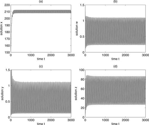
, we can get Figure ; If
, we can get Figure . From Figures and , we can know that Theorem 4.3 holds.
Figure 1. Numerical simulations show that the equilibrium of system (12) is locally asymptotically stable when
holds.
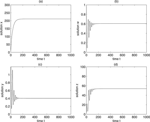
Figure 2. Numerical simulations show that the equilibrium of system (12) is unstable when
holds.
6. Conclusion and prospects
In this paper, we established a mathematical model for HIV-1 with the immune delay and Holling II infection rate. In this model, we define the infection of the basic reproductive number and the basic immune response reproductive number
by calculating and we identify the three equilibrium of the model. Then, it will show that uninfected equilibrium
of system (Equation2
(2)
(2) ) is globally asymptotically stable for any time delay
by using the Lyapunov–LaSalle theorem when the infection of the basic reproductive number
; the infected equilibrium without immune response of system (Equation2
(2)
(2) ) is globally asymptotical stable for any time delay
, when
and
hold; the infected equilibrium with immune response
of system (Equation2
(2)
(2) ) is globally stable for
, when
and
hold. And we also give sufficient condition of the Hopf bifurcation in equilibrium
of system (Equation2
(2)
(2) ). Our analysis provides the effective reference value of the prevention and treatment of AIDS.
By using a novel reducing dimension modelling idea proposed in [Citation29], see also [Citation30, Citation31], we may reduce (Equation2(2)
(2) ) into a three dimension system if we regard
or
as a known function rather than an independent variable satisfying an independent dynamical equation, which will be a challenging topic to the future study.
Disclosure statement
No potential conflict of interest was reported by the author(s).
Additional information
Funding
References
- B. Buonomo and C. Vargas-De-Leon, Global stability for an HIV-1 infection model including an eclipse stage of infected cells, J. Math. Anal. Appl. 385 (2012), pp. 709–720.
- A.A. Canabarro, I.M. Gleria, and M.L. Lyra, Periodic solutions and chaos in a nonlinear model for the delayed cellular immune response, Physica 342 (2004), pp. 232–241.
- D. Ebert, C.D. Zschokke-Rohringer, and H.J. Carins, Does effects and density dependent regulation of two microparasites of Daphnia magna, Oecologia 122 (2000), pp. 200–209.
- P. Essunger and A.S. Perelson, Modeling HIV infection of CD4+T cell subpopulations, J. Theor. Biol.170 (1994), pp. 367–391.
- Q.M. Gou and W.D. Wang, Global stability of an SEIS Epidemic model with saturating incidence, J. Biomath. 23 (2008), pp. 265–272.
- B.D. Hassard, N.D. Kazarinoff, and Y.H. wan, Theory and Applications of Hopf Bifurcation, Cambridge University Press, Cambridge, 1981.
- G. Huang, H. Yokoi, Y. Takeuchi, T. Kajiwara, and T. Sasaki, Impact of intracellular delay, immune activation delay and nonlinear incidence on viral dynamics, Jpn J. Ind. Appl. Math. 28 (2011), pp. 383–411.
- A. Korobeinikov, Global properties of basic virus dynamics models, Bull. Math. Biol. 66(4) (2004), pp. 879–883.
- A. Korobeinikov, Global asymptotic properties of virus dynamics models with dose dependent parasite reproduction and virulence, and nonlinear incidence rate, Math. Medi. Biol. 26 (2009), pp. 225–239.
- S. Liu, X. Pan, and W. Zhao, HIV cure: latent HIV eradication and strategies, Journal of Zunyi Medical University 38(2) (2015), pp. 105–110.
- S. Liu and L. Wang, Global stability of an HIV-1 model with distributed intracellular delays and a combination therapy, Math. Biosci. 7 (2010), pp. 675–685.
- X.D. Liu, H. Wang, Z.X. Hu, and W. Ma, Global stability of an HIV pathogenesis model with cure rate, Nonlinear Anal. Real World Appl. 12 (2011), pp. 2947–2961.
- C.F. Lv, L.H. Huang, and Z.H. Yuan, Global stability for an HIV-1 infection model with Beddington-DeAngelis incidence rate and CTL immune response, Commun. Nonlinear Sci. Numer. Simul. 19 (2014), pp. 121–127.
- M. Nasri, M. Dehghan, and M. Jaberi Douraki, Study of a system of non-linear difference equations arising in a deterministic model for HIV infection, Appl. Math. Comput. 171 (2005), pp. 1306–1330.
- L. Rong, M. A. Gilchrist, Z. Feng, and A. S. Perelson, Modeling within-host HIV-1 dynamics and the evolution of drug resistance: trade-offs between viral enzyme function and drug susceptibility, J. Theor. Biol. 247 (2007), pp. 804–818.
- L. Rong and A. S. Perelson, Asymmetric division of activated latently infected cells may explain the decay kinetics of the HIV-1 latent reservoir and intermittent viral blips, Math. Biosci. 217(1) (2009), pp. 77–87.
- M.W. Shen, Y.N. Xiao, and L.B. Rong, Global stability of an infection-age structured HIV-1 model linking within-host and between-host dynamics, Math. Biosci. 263 (2015), pp. 37–50.
- C. Sun, L. Li, and J. Jia, Hopf bifurcation of an HIV-1 virus model with two delays and logistic growth, Math. Model. Nat. Pheno. 15 (2020), pp. 16–20.
- E. Vicenzi and G. Poli, Novel factors interfering with human immunodeficiency virus - type 1 replication in vivo and in vitro, Tissue Antigens 81(2) (2013), pp. 61–71.
- K.F. Wang, W.D. Wang, H.Y. Pang, and X. Liu, Complex dynamic behavior in a viral model with delayed immune response, Physica D. 226 (2007), pp. 197–208.
- X. Wang, A. Elaiw, and X.Y. Song, Global properties of a delayed HIV infection model with CTL immune response, Appl. Math. Comput. 218 (2012), pp. 9405–9414.
- C.J. Xu, Local and global Hopf bifurcation analysis on simplified bidirectional associative memory neural networks with multiple delays, Math. Comput. Simulat. 149 (2018), pp. 69–90.
- R. Xu, Global dynamics of an HIV-1 infection model with distributed intracellular delays, Comput. Math. Appl. 61 (2011), pp. 2799–2805.
- R. Xu, Global stability of an HIV-1 infection model with saturation infection and intracellular delay, J. Math. Anal. Appl. 375 (2011), pp. 75–81.
- C.J. Xu and C. Aouiti, Comparative analysis on Hopf bifurcation of integer order and fractional order two-neuron neural networks with delay, Int. J. Circuit Theory Appl. 48(9) (2020), pp. 1459–1475.
- C.J. Xu, C. Aouiti, and Z. Liu, A further study on bifurcation for fractional order BAM neural networks with multiple delays, Neurocomputing 417 (2020), pp. 501–515.
- C.J. Xu, M. Liao, P. Li, Y. Guo, and S. Yuan, Influence of multiple time delays on bifurcation of fractional-order neural networks, Appl. Math. Comput. 361 (2019), pp. 565–582.
- C.J. Xu and Q. Zhang, Bifurcation analysis of a tri-neuron neural network model in the frequency domain, Nonlinear Dyn. 76(1) (2014), pp. 33–46.
- J.S. Yu, Modeling mosquito population suppression based on delay differential equations, SIAM J. Appl. Math. 78 (2018), pp. 3168–3187.
- J.S. Yu, Existence and stability of a unique and exact two periodic orbits for an interactive wild and sterile mosquito model, J. Differ. Equ. 269 (2020), pp. 10395–10415.
- J.S. Yu and J. Li, Global asymptotic stability in an interactive wild and sterile mosquito model, J. Differ. Equ. 269 (2020), pp. 6193–6215.
- Z.H. Yuan, Z.J. Ma, and X.H. Tang, Global stability of a delayed HIV infection model with nonlinear incidence rate, Nonlinear Dyn. 68 (2012), pp. 207–214.
- R. Zhang and S. Liu, Global dynamics of an age-structured within-host viral infection model with cell-to-cell transmission and general humoral immunity response, Math. Biosci. Eng. 17(2) (2020), pp. 1450–1478.