Delay in budget allocation for vaccination and awareness induces chaos in an infectious disease model

Abstract

In this paper, we propose a model to assess the impacts of budget allocation for vaccination and awareness programs on the dynamics of infectious diseases. The budget allocation is assumed to follow logistic growth, and its per capita growth rate increases proportional to disease prevalence. An increment in per-capita growth rate of budget allocation due to increase in infected individuals after a threshold value leads to onset of limit cycle oscillations. Our results reveal that the epidemic potential can be reduced or even disease can be eradicated through vaccination of high quality and/or continuous propagation of awareness among the people in endemic zones. We extend the proposed model by incorporating a discrete time delay in the increment of budget allocation due to infected population in the region. We observe that multiple stability switches occur and the system becomes chaotic on gradual increase in the value of time delay.

Keywords:

• Budget allocation
• vaccination
• awareness
• sensitivity
• time delay
• chaos

1. Introduction

Infectious diseases are major threat to mankind, and are responsible for hindrance in social and economic development of any country. Vaccination coverage is one of the most powerful and cost-effective intervention to reduce the prevalence of disease. It saves countless lives and prevents an estimated 2.5 million deaths each year caused by whooping cough, influenza, measles, etc., [54]. The global health communities, such as Global Alliance of Vaccination and Immunization (GAVI), Bill & Melinda Gates Foundation, and other government and non-government organizations of various countries are making much efforts to make the vaccines accessible to all the people across the globe. These non-profitable organizations along with government provide funds for vaccination and awareness as the underprivileged people do not have sufficient amount of money to go for self-financed vaccination and also lack of awareness regarding the vaccination campaigns. As a result, they deprive from the health benefit provided by the government and thus are at the risk of infection during the infection period. The public perception of the possible risks and misconception associated with vaccination has led to reduction in MMR vaccine uptake, resulting the re-emergence of measles epidemic in the UK [25]. In this regard, the global information campaigns via TV, radio and social media (accessible to most of the population) play a crucial role to convey the important health messages to unaware people and inform them how immunizations help to save their lives.

Several studies have been conducted to assess the impact of vaccination coverage to control the spread of infectious diseases [4, 6–8, 11, 14, 26, 27, 41, 45, 51, 52, 55]. The combined effects of education, vaccination and treatment are proven to be more effective to reduce the prevalence of HIV in comparison to the case when only one of them is applied [11]. Agaba et al. [1] have investigated the role of vaccination on the dynamics of infectious disease in presence of global information campaigns regarding the disease prevalence as well as local awareness due to direct interaction between unaware and aware individuals. It is observed that the delay in response to available information about the disease leads to destabilization of endemic state and the periodic oscillations arise. Their findings suggest that vaccination coverage in the presence of awareness is helpful to reduce the size of epidemic.

Although vaccination coverage is crucial for public health (as it triggers the immune response by developing antibodies), the awareness programs through TV, radio (a cost-effective and responsive medium in remote areas) and social media are also helpful in reducing the disease transmission by alerting the people to adopt practices that are requisite for disease prevention, such as go for vaccination, adopt sanitation practices, use of face mask, etc. The implementation of effective control strategies is beneficial to suppress the burden of disease. For instance, Guinea worm disease is eradicated only through proper program implementation strategies [18]. Some mathematical studies are carried out to see the impact of awareness for the control of disease transmission. Authors considered media as a dynamic variable and assumed that awareness programs increase with the increase in the number of infected individuals [15, 24, 32, 34, 37, 38, 43, 44, 46, 48, 50] or transmission rate decreases with the increase in infected individuals due to awareness [2, 10, 30, 40, 47, 49]. In [38], the effect of behavioural changes induced by information campaigns for the control of infectious diseases by considering prevalence-dependent information campaigns is investigated. The study reveals that optimal media campaigns are effective and economical to control an epidemic. The findings of Huo et al. [24] suggested that media serves as a good indicator during an epidemic outbreak and is helpful in reducing the disease burden. Misra and Rai [33] have shown that the broadcastings via TV and radio regarding the control mechanisms are beneficial to reduce the spread of infectious diseases. The global information campaigns through TV, radio and social media encourage people to adopt preventive measures at the early stage of epidemic outbreak that helps to suppress the burden of disease. The other key tools to prevent a disease are medical health facilities, public health responses, health infrastructures, public education, vaccination coverage, etc. On the other hand, media has some negative effects as well. For example, the negative effects of media at the time of the plague outbreak in India during 1994 largely affected tourism and other businesses [13]. The epicentre of plague was Surat, Gujarat; in total, 52 people died. Although, the plague lasted in two weeks but a large number of people left the city due to media-induced panic.

Some mathematical models are also proposed to assess the effect of time delay in implementation of awareness programs [1, 3, 20, 35, 36]. It is observed that such time lag destabilizes the system via Hopf-bifurcation. Basir et al. [3] have investigated the role of awareness programs on the control of infectious diseases. They observed that the incorporation of time delay in implementation of information campaigns and/or response of unaware (aware) susceptible individuals to become aware (unaware) destabilizes the system and periodic oscillations arise through Hopf-bifurcation. Their study shows that media campaigns influence the patterns of disease and also help to reduce the risk of infection. Misra et al. [35] have also studied a nonlinear mathematical model to see how the introduction of delay in per-capita growth rate of budget allocation changes the dynamics of system. They observed that the propagation of awareness reduces the disease burden but the delay in providing funds destabilizes the system and may cause stability switches through Hopf-bifurcation. Their findings suggest that the continuous and timely allocation of funds are beneficial to reduce the disease prevalence.

Rai et al. [43] have explored the combined actions of awareness and sanitation on the spread of infectious diseases. Their findings revealed that the sanitation and awareness programs have capability to reduce the epidemic threshold, and thus control the spread of infection. In the present paper, we investigate the impacts of vaccination coverage and information campaigns on the control of disease prevalence. Our model is different from the model proposed by Rai et al. [43] in the following sense. In the present study, our goal is to assess the joint impacts of vaccination (a powerful and cost-effective intervention to protect the people against contracting the disease) and non-pharmaceutical interventions such as frequent hand washing, use of face mask, sanitizer, maintain social distancing, etc., induced by the information campaigns to control infectious diseases, which spread in the population through the direct contact with infected individuals, such as influenza, measles, etc., in the presence of budget allocation. On the other hand, Rai et al. [43] have explicitly incorporated the combined effects of sanitation coverage (a rational step for the control of bacteria present in the environment) and awareness programs through budget allocation for the control of infectious diseases, such as typhoid fever which spreads in the population through the direct contact of susceptible with infected individuals as well as indirectly through bacteria present in the environment. Here, our aim is to explore whether disease can be eliminated by vaccination coverage and/or awareness programs. We also investigate the impact of time delay involved in the increment in budget allocation due to increased number of infected individuals.

The rest of the paper is arranged as follows: in the next section, we propose our model. In Section 3, we obtain equilibria of the system and study their stability behaviour. We find expression for the basic reproduction number, and investigate the direction of bifurcation whenever basic reproduction number is unity. Existence of Hopf-bifurcation is discussed with respect to the per-capita growth rate of budget allocation due to increased population of infectives; we also determine the conditions for direction and stability of bifurcating periodic solutions. In Section 4, we extend our model by considering the effect of time delay in the increments in budget allocation due to increased infected population. The delay system is analysed in the following section. We simulate our delay and non-delay systems in Section 6. Section 7 contains our conclusion.

2. Mathematical model

In the region under consideration, let $N\left(t\right)$ be the total population at any time t>0, which is divided into three sub-populations: susceptible individuals $S\left(t\right)$, infected individuals $I\left(t\right)$ and vaccinated individuals $V\left(t\right)$. Further, we denote by $M\left(t\right)$, the budget allocation by the government for vaccination and awareness in the region at time t. In the modelling process, it is assumed that the growth rate of budget allocation regarding the protection against the disease follows the logistic growth with intrinsic growth rate r and carrying capacity K, and its per-capita growth rate increases in proportion to the number of infected individuals. It is assumed that the population is homogeneously mixed and the susceptible individuals contract the infection through the direct contact with infected individuals at the contact rate β. The interaction between susceptible and infected individuals is assumed to follow the simple law of mass action.

We assume that $k_1$ fraction of the total allocated budget M (i.e. $k_{1}M$, $0<k_1<1$) is used to warn people via propagating awareness regarding the risk of infection and its control mechanisms. As a result, the individuals change their behaviours and use precautionary measures during the infection period. Thus, the direct contact between susceptible and infected individuals decreases at a factor ${\displaystyle f_1\left(M\right)={\text{β}}_1\frac{k_{1}M}{p+k_{1}M}.}$ The reason behind considering this saturated type of functional response is that the amount of funds used to propagate awareness has limited impact to reduce the possibility of contracting the infection [30]. Due to this, the effective contact between susceptible and infected individuals becomes ${\displaystyle \text{β}\left(M\right)=\text{β}-{\text{β}}_1\frac{k_{1}M}{p+k_{1}M}.}$ Further, the remaining part of budget, i.e. $(1-k_1)M$ is used for vaccination coverage; the effective vaccination rate of susceptible individuals in the presence of budget is ${\displaystyle f_2\left(M\right)=\varphi \frac{(1-k_1)M}{q+(1-k_1)M}.}$ Again, a saturated type of functional response is considered here because of the cost and efficacy of the vaccines. Moreover, the vaccine is not fully effective and it wears off after certain period of time. After recovery, the infected individuals are assumed to join the susceptible class again. Individuals in each class have natural mortality while the individuals in the infected class also experience disease induced death.

In view of above assumptions, a schematic diagram for the proposed system is depicted in Figure 1, and the model equations are written as follows: (1) $\begin{array}{rl}\frac{\mathrm{d}S}{\mathrm{d}t}& =\mathrm{\Lambda }-\left(\text{β}-{\text{β}}_1\frac{k_{1}M}{p+k_{1}M}\right)SI-\varphi \frac{(1-k_1)M}{q+(1-k_1)M}S+\nu I+\delta V-\mathrm{d}S,\\ \frac{\mathrm{d}I}{\mathrm{d}t}& =\left(\text{β}-{\text{β}}_1\frac{k_{1}M}{p+k_{1}M}\right)SI-(\nu +\alpha +d)I,\\ \frac{\mathrm{d}V}{\mathrm{d}t}& =\varphi \frac{(1-k_1)M}{q+(1-k_1)M}S-(\delta +d)V,\\ \frac{\mathrm{d}M}{\mathrm{d}t}& =rM\left(1-\frac{M}{K}\right)+\theta IM.\end{array}$(1) The initial conditions are assumed as, $S\left(0\right)>0,I\left(0\right)\ge 0,V\left(0\right)\ge 0,M\left(0\right)\ge 0.$For the feasibility of system (1(1) $\begin{array}{rl}\frac{\mathrm{d}S}{\mathrm{d}t}& =\mathrm{\Lambda }-\left(\text{β}-{\text{β}}_1\frac{k_{1}M}{p+k_{1}M}\right)SI-\varphi \frac{(1-k_1)M}{q+(1-k_1)M}S+\nu I+\delta V-\mathrm{d}S,\\ \frac{\mathrm{d}I}{\mathrm{d}t}& =\left(\text{β}-{\text{β}}_1\frac{k_{1}M}{p+k_{1}M}\right)SI-(\nu +\alpha +d)I,\\ \frac{\mathrm{d}V}{\mathrm{d}t}& =\varphi \frac{(1-k_1)M}{q+(1-k_1)M}S-(\delta +d)V,\\ \frac{\mathrm{d}M}{\mathrm{d}t}& =rM\left(1-\frac{M}{K}\right)+\theta IM.\end{array}$(1) ), we must have ${\text{β}}_1<\text{β}$. All the parameters involved in system (1(1) $\begin{array}{rl}\frac{\mathrm{d}S}{\mathrm{d}t}& =\mathrm{\Lambda }-\left(\text{β}-{\text{β}}_1\frac{k_{1}M}{p+k_{1}M}\right)SI-\varphi \frac{(1-k_1)M}{q+(1-k_1)M}S+\nu I+\delta V-\mathrm{d}S,\\ \frac{\mathrm{d}I}{\mathrm{d}t}& =\left(\text{β}-{\text{β}}_1\frac{k_{1}M}{p+k_{1}M}\right)SI-(\nu +\alpha +d)I,\\ \frac{\mathrm{d}V}{\mathrm{d}t}& =\varphi \frac{(1-k_1)M}{q+(1-k_1)M}S-(\delta +d)V,\\ \frac{\mathrm{d}M}{\mathrm{d}t}& =rM\left(1-\frac{M}{K}\right)+\theta IM.\end{array}$(1) ) are assumed to be positive, and their descriptions are given in Table 1.

Figure 1. Schematic diagram for systems (1(1) $\begin{array}{rl}\frac{\mathrm{d}S}{\mathrm{d}t}& =\mathrm{\Lambda }-\left(\text{β}-{\text{β}}_1\frac{k_{1}M}{p+k_{1}M}\right)SI-\varphi \frac{(1-k_1)M}{q+(1-k_1)M}S+\nu I+\delta V-\mathrm{d}S,\\ \frac{\mathrm{d}I}{\mathrm{d}t}& =\left(\text{β}-{\text{β}}_1\frac{k_{1}M}{p+k_{1}M}\right)SI-(\nu +\alpha +d)I,\\ \frac{\mathrm{d}V}{\mathrm{d}t}& =\varphi \frac{(1-k_1)M}{q+(1-k_1)M}S-(\delta +d)V,\\ \frac{\mathrm{d}M}{\mathrm{d}t}& =rM\left(1-\frac{M}{K}\right)+\theta IM.\end{array}$(1) ) and (16(16) $\begin{array}{rl}\frac{\mathrm{d}I}{\mathrm{d}t}& =\left(\text{β}-{\text{β}}_1\frac{k_{1}M}{p+k_{1}M}\right)(N-I-V)I-(\nu +\alpha +d)I,\\ \frac{\mathrm{d}V}{\mathrm{d}t}& =\frac{\varphi (1-k_1)M}{q+(1-k_1)M}(N-I-V)-(\delta +d)V,\\ \frac{\mathrm{d}N}{\mathrm{d}t}& =\mathrm{\Lambda }-\mathrm{d}N-\alpha I,\\ \frac{\mathrm{d}M}{\mathrm{d}t}& =rM\left(1-\frac{M}{K}\right)+\theta I(t-\tau )M.\end{array}$(16) ). Here, red colour denotes the impact of budget allocation in reducing the transmission rate by making people aware about the disease whereas blue colour stands for the utilization of budget on vaccinating the susceptible individuals; time delay involved in per-capita growth rate of budget allocation due to increase in infected individuals is represented by cyan colour.

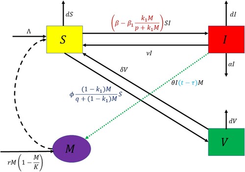
Table 1. Descriptions of parameters involved in system (1(1) $\begin{array}{rl}\frac{\mathrm{d}S}{\mathrm{d}t}& =\mathrm{\Lambda }-\left(\text{β}-{\text{β}}_1\frac{k_{1}M}{p+k_{1}M}\right)SI-\varphi \frac{(1-k_1)M}{q+(1-k_1)M}S+\nu I+\delta V-\mathrm{d}S,\\ \frac{\mathrm{d}I}{\mathrm{d}t}& =\left(\text{β}-{\text{β}}_1\frac{k_{1}M}{p+k_{1}M}\right)SI-(\nu +\alpha +d)I,\\ \frac{\mathrm{d}V}{\mathrm{d}t}& =\varphi \frac{(1-k_1)M}{q+(1-k_1)M}S-(\delta +d)V,\\ \frac{\mathrm{d}M}{\mathrm{d}t}& =rM\left(1-\frac{M}{K}\right)+\theta IM.\end{array}$(1) ).

Parameters	Descriptions	Units	Values	Sources
Λ	Immigration into the class of susceptible	person day${}^{-1}$	2	Assumed
	population
β	Contact rate of susceptible with	person${}^{-1}$day${}^{-1}$	0.000024	Assumed
	infected individuals in absence of funds
${\text{β}}_1$	Efficacy of budget allocation to reduce	person${}^{-1}$day${}^{-1}$	0.000012	[35]
	the contact rate via propagating awareness
$k_1$	Fraction of budget allocated to	–	0.4	Assumed
	warn susceptibles via propagating awareness
p	Half saturation constant	dollar	50	Assumed
ϕ	Vaccination rate among susceptible individuals	day${}^{-1}$	0.004	Assumed
	in the presence of budget allocation
q	Half saturation constant	dollar	150	Assumed
δ	Rate of transfer of vaccinated individuals to	day${}^{-1}$	0.003	Assumed
	susceptible class due to ineffectiveness of vaccine
ν	Recovery rate of human population	day${}^{-1}$	0.34	[29]
α	Disease-induced death rate of human population	day${}^{-1}$	0.0002	Assumed
d	Natural death rate of human population	day${}^{-1}$	0.00004	[17]
r	Intrinsic growth rate of budget allocation	day${}^{-1}$	0.5	Assumed
K	Carrying capacity of budget allocation	dollar	500	Assumed
θ	Per-capita growth rate of budget allocation due	person${}^{-1}$day${}^{-1}$	0.0005	Assumed
	to increase in infected individuals

As S + I + V = N, system (1(1) $\begin{array}{rl}\frac{\mathrm{d}S}{\mathrm{d}t}& =\mathrm{\Lambda }-\left(\text{β}-{\text{β}}_1\frac{k_{1}M}{p+k_{1}M}\right)SI-\varphi \frac{(1-k_1)M}{q+(1-k_1)M}S+\nu I+\delta V-\mathrm{d}S,\\ \frac{\mathrm{d}I}{\mathrm{d}t}& =\left(\text{β}-{\text{β}}_1\frac{k_{1}M}{p+k_{1}M}\right)SI-(\nu +\alpha +d)I,\\ \frac{\mathrm{d}V}{\mathrm{d}t}& =\varphi \frac{(1-k_1)M}{q+(1-k_1)M}S-(\delta +d)V,\\ \frac{\mathrm{d}M}{\mathrm{d}t}& =rM\left(1-\frac{M}{K}\right)+\theta IM.\end{array}$(1) ) reduces to following equivalent system: (2) $\begin{array}{rl}\frac{\mathrm{d}I}{\mathrm{d}t}& =\left(\text{β}-{\text{β}}_1\frac{k_{1}M}{p+k_{1}M}\right)(N-I-V)I-(\nu +\alpha +d)I,\\ \frac{\mathrm{d}V}{\mathrm{d}t}& =\varphi \frac{(1-k_1)M}{q+(1-k_1)M}(N-I-V)-(\delta +d)V,\\ \frac{\mathrm{d}N}{\mathrm{d}t}& =\mathrm{\Lambda }-\mathrm{d}N-\alpha I,\\ \frac{\mathrm{d}M}{\mathrm{d}t}& =rM\left(1-\frac{M}{K}\right)+\theta IM.\end{array}$(2) Now onwards, we study the dynamics of system (2(2) $\begin{array}{rl}\frac{\mathrm{d}I}{\mathrm{d}t}& =\left(\text{β}-{\text{β}}_1\frac{k_{1}M}{p+k_{1}M}\right)(N-I-V)I-(\nu +\alpha +d)I,\\ \frac{\mathrm{d}V}{\mathrm{d}t}& =\varphi \frac{(1-k_1)M}{q+(1-k_1)M}(N-I-V)-(\delta +d)V,\\ \frac{\mathrm{d}N}{\mathrm{d}t}& =\mathrm{\Lambda }-\mathrm{d}N-\alpha I,\\ \frac{\mathrm{d}M}{\mathrm{d}t}& =rM\left(1-\frac{M}{K}\right)+\theta IM.\end{array}$(2) ) in detail.

Lemma 2.1

The following set contains the region of attraction for the system (2(2) $\begin{array}{rl}\frac{\mathrm{d}I}{\mathrm{d}t}& =\left(\text{β}-{\text{β}}_1\frac{k_{1}M}{p+k_{1}M}\right)(N-I-V)I-(\nu +\alpha +d)I,\\ \frac{\mathrm{d}V}{\mathrm{d}t}& =\varphi \frac{(1-k_1)M}{q+(1-k_1)M}(N-I-V)-(\delta +d)V,\\ \frac{\mathrm{d}N}{\mathrm{d}t}& =\mathrm{\Lambda }-\mathrm{d}N-\alpha I,\\ \frac{\mathrm{d}M}{\mathrm{d}t}& =rM\left(1-\frac{M}{K}\right)+\theta IM.\end{array}$(2) ) with initial conditions $I\left(0\right)\ge 0,$ $V\left(0\right)\ge 0,$ $N\left(0\right)>0$ and $M\left(0\right)\ge 0,$ and attracts all solutions initiating in the interior of positive orthant: $\mathrm{\Omega }=\left\{(I,V,N,M)\in {\mathbb{R}}_{+}^4:0\le I,V\le N\le \frac{\mathrm{\Lambda }}{d},0\le M\le \frac{K}{r}\left(r+\theta \frac{\mathrm{\Lambda }}{d}\right)=M_r\right\}.$

3. Mathematical analysis of system (2)

3.1. Equilibrium analysis

System (2(2) $\begin{array}{rl}\frac{\mathrm{d}I}{\mathrm{d}t}& =\left(\text{β}-{\text{β}}_1\frac{k_{1}M}{p+k_{1}M}\right)(N-I-V)I-(\nu +\alpha +d)I,\\ \frac{\mathrm{d}V}{\mathrm{d}t}& =\varphi \frac{(1-k_1)M}{q+(1-k_1)M}(N-I-V)-(\delta +d)V,\\ \frac{\mathrm{d}N}{\mathrm{d}t}& =\mathrm{\Lambda }-\mathrm{d}N-\alpha I,\\ \frac{\mathrm{d}M}{\mathrm{d}t}& =rM\left(1-\frac{M}{K}\right)+\theta IM.\end{array}$(2) ) exhibits four non-negative equilibria, which are listed as follows.

1. The disease and budget-free equilibrium (DBFE) $E_1=(0,0,\mathrm{\Lambda }/d,0)$, which always exists.

2. The budget-free endemic equilibrium (BFEE) $E_2=(I_2,0,N_2,0)$, where (3) $I_2=\frac{\text{β}\mathrm{\Lambda }-d(\nu +\alpha +d)}{\text{β}(\alpha +d)},N_2=\frac{\text{β}\mathrm{\Lambda }+\alpha (\nu +\alpha +d)}{\text{β}(\alpha +d)}.$(3) The equilibrium $E_2$ exists provided ${\mathcal{R}}_0>1$, where (4) ${\mathcal{R}}_0=\frac{\text{β}\mathrm{\Lambda }}{d(\nu +\alpha +d)}.$(4)

3. The disease-free equilibrium (DFE) $E_3=(0,V_3,\mathrm{\Lambda }/d,K)$, where $V_3=\frac{\varphi \mathrm{\Lambda }}{d}\frac{(1-k_1)K}{q+(1-k_1)K}{\left[\varphi \frac{(1-k_1)K}{q+(1-k_1)K}+\delta +d\right]}^{-1}.$This equilibrium always exists.

4. The interior equilibrium (IE) $E^{\ast }=(I^{\ast },V^{\ast },N^{\ast },M^{\ast })$, where the values of $I^{\ast }$, $V^{\ast }$, $N^{\ast }$ and $M^{\ast }$ are positive solutions of the equilibrium equations of system (2(2) $\begin{array}{rl}\frac{\mathrm{d}I}{\mathrm{d}t}& =\left(\text{β}-{\text{β}}_1\frac{k_{1}M}{p+k_{1}M}\right)(N-I-V)I-(\nu +\alpha +d)I,\\ \frac{\mathrm{d}V}{\mathrm{d}t}& =\varphi \frac{(1-k_1)M}{q+(1-k_1)M}(N-I-V)-(\delta +d)V,\\ \frac{\mathrm{d}N}{\mathrm{d}t}& =\mathrm{\Lambda }-\mathrm{d}N-\alpha I,\\ \frac{\mathrm{d}M}{\mathrm{d}t}& =rM\left(1-\frac{M}{K}\right)+\theta IM.\end{array}$(2) ).

   From the third equilibrium equation of system (2(2) $\begin{array}{rl}\frac{\mathrm{d}I}{\mathrm{d}t}& =\left(\text{β}-{\text{β}}_1\frac{k_{1}M}{p+k_{1}M}\right)(N-I-V)I-(\nu +\alpha +d)I,\\ \frac{\mathrm{d}V}{\mathrm{d}t}& =\varphi \frac{(1-k_1)M}{q+(1-k_1)M}(N-I-V)-(\delta +d)V,\\ \frac{\mathrm{d}N}{\mathrm{d}t}& =\mathrm{\Lambda }-\mathrm{d}N-\alpha I,\\ \frac{\mathrm{d}M}{\mathrm{d}t}& =rM\left(1-\frac{M}{K}\right)+\theta IM.\end{array}$(2) ), we get (5) $N=\frac{\mathrm{\Lambda }-\alpha I}{d}.$(5) From the last equilibrium equation of system (2(2) $\begin{array}{rl}\frac{\mathrm{d}I}{\mathrm{d}t}& =\left(\text{β}-{\text{β}}_1\frac{k_{1}M}{p+k_{1}M}\right)(N-I-V)I-(\nu +\alpha +d)I,\\ \frac{\mathrm{d}V}{\mathrm{d}t}& =\varphi \frac{(1-k_1)M}{q+(1-k_1)M}(N-I-V)-(\delta +d)V,\\ \frac{\mathrm{d}N}{\mathrm{d}t}& =\mathrm{\Lambda }-\mathrm{d}N-\alpha I,\\ \frac{\mathrm{d}M}{\mathrm{d}t}& =rM\left(1-\frac{M}{K}\right)+\theta IM.\end{array}$(2) ), we have (6) $M=\frac{K}{r}(r+\theta I).$(6) We have, (7) $g\left(I\right)=\frac{(1-k_1)M}{q+(1-k_1)M}=\frac{(1-k_1)K(r+\theta I)}{qr+(1-k_1)K(r+\theta I)}.$(7) Note that, $g^{\mathrm{\prime }}\left(I\right)=\frac{qr(1-k_1)K\theta }{[qr+(1-k_1\left)K\right(r+\theta I){]}^2}>0.$Using Equations (5(5) $N=\frac{\mathrm{\Lambda }-\alpha I}{d}.$(5) )–(7(7) $g\left(I\right)=\frac{(1-k_1)M}{q+(1-k_1)M}=\frac{(1-k_1)K(r+\theta I)}{qr+(1-k_1)K(r+\theta I)}.$(7) ) in the second equilibrium equation of system (2(2) $\begin{array}{rl}\frac{\mathrm{d}I}{\mathrm{d}t}& =\left(\text{β}-{\text{β}}_1\frac{k_{1}M}{p+k_{1}M}\right)(N-I-V)I-(\nu +\alpha +d)I,\\ \frac{\mathrm{d}V}{\mathrm{d}t}& =\varphi \frac{(1-k_1)M}{q+(1-k_1)M}(N-I-V)-(\delta +d)V,\\ \frac{\mathrm{d}N}{\mathrm{d}t}& =\mathrm{\Lambda }-\mathrm{d}N-\alpha I,\\ \frac{\mathrm{d}M}{\mathrm{d}t}& =rM\left(1-\frac{M}{K}\right)+\theta IM.\end{array}$(2) ), we get (8) $V=\frac{\varphi g\left(I\right)\{\mathrm{\Lambda }-(\alpha +d\left)I\right\}}{d\left\{\varphi g\right(I)+\delta +d\}}.$(8) Now, using Equations (5(5) $N=\frac{\mathrm{\Lambda }-\alpha I}{d}.$(5) ), (6(6) $M=\frac{K}{r}(r+\theta I).$(6) ) and (8(8) $V=\frac{\varphi g\left(I\right)\{\mathrm{\Lambda }-(\alpha +d\left)I\right\}}{d\left\{\varphi g\right(I)+\delta +d\}}.$(8) ) in the first equilibrium equation of system (2(2) $\begin{array}{rl}\frac{\mathrm{d}I}{\mathrm{d}t}& =\left(\text{β}-{\text{β}}_1\frac{k_{1}M}{p+k_{1}M}\right)(N-I-V)I-(\nu +\alpha +d)I,\\ \frac{\mathrm{d}V}{\mathrm{d}t}& =\varphi \frac{(1-k_1)M}{q+(1-k_1)M}(N-I-V)-(\delta +d)V,\\ \frac{\mathrm{d}N}{\mathrm{d}t}& =\mathrm{\Lambda }-\mathrm{d}N-\alpha I,\\ \frac{\mathrm{d}M}{\mathrm{d}t}& =rM\left(1-\frac{M}{K}\right)+\theta IM.\end{array}$(2) ), we get (9) $\begin{array}{rl}F\left(I\right)& =\left(\text{β}-{\text{β}}_1\frac{k_{1}K(r+\theta I)}{pr+k_{1}K(r+\theta I)}\right)\frac{(\delta +d)\{\mathrm{\Lambda }-(\alpha +d\left)I\right\}}{d\left\{\varphi g\right(I)+\delta +d\}}\\ & -(\nu +\alpha +d)=0.\end{array}$(9) Form Equation (9(9) $\begin{array}{rl}F\left(I\right)& =\left(\text{β}-{\text{β}}_1\frac{k_{1}K(r+\theta I)}{pr+k_{1}K(r+\theta I)}\right)\frac{(\delta +d)\{\mathrm{\Lambda }-(\alpha +d\left)I\right\}}{d\left\{\varphi g\right(I)+\delta +d\}}\\ & -(\nu +\alpha +d)=0.\end{array}$(9) ), we observe that

   1. $\begin{array}{rl}F\left(0\right)& =\left(\text{β}-{\text{β}}_1\frac{k_{1}K}{p+k_{1}K}\right)\frac{\mathrm{\Lambda }(\delta +d)}{d}{\left[\varphi \frac{(1-k_1)K}{q+(1-k_1)K}+\delta +d\right]}^{-1}\\ & -(\nu +\alpha +d),\end{array}$which is positive provided ${\mathcal{R}}_{\mathrm{a}\mathrm{v}}>1$, where ${\mathcal{R}}_{\mathrm{a}\mathrm{v}}$ is defined in (10(10) ${\mathcal{R}}_{\mathrm{a}\mathrm{v}}=\left(\text{β}-{\text{β}}_1\frac{k_{1}K}{p+k_{1}K}\right)\frac{\mathrm{\Lambda }(\delta +d)}{d(\nu +\alpha +d)}{\left[\varphi \frac{(1-k_1)K}{q+(1-k_1)K}+\delta +d\right]}^{-1}.$(10) ).

   2. ${\displaystyle F\left(\frac{\mathrm{\Lambda }}{\alpha +d}\right)=-(\nu +\alpha +d)<0.}$

   3. $F^{\mathrm{\prime }}\left(I\right)<0$ for all ${\displaystyle I\in \left(0,\frac{\mathrm{\Lambda }}{\alpha +d}\right).}$

   Thus, $F\left(I\right)=0$ has a unique positive root, say $I^{\ast }$ in the open interval ${\displaystyle \left(0,\frac{\mathrm{\Lambda }}{\alpha +d}\right)}$ provided ${\mathcal{R}}_{\mathrm{a}\mathrm{v}}>1$. Now, using this positive value of $I=I^{\ast }$ in Equations (5(5) $N=\frac{\mathrm{\Lambda }-\alpha I}{d}.$(5) ), (6(6) $M=\frac{K}{r}(r+\theta I).$(6) ) and (8(8) $V=\frac{\varphi g\left(I\right)\{\mathrm{\Lambda }-(\alpha +d\left)I\right\}}{d\left\{\varphi g\right(I)+\delta +d\}}.$(8) ), we can obtain the positive values of $N^{\ast }$, $M^{\ast }$ and $V^{\ast }$, respectively.

3.2. Basic reproduction number

To obtain the basic reproduction number (${\mathcal{R}}_{\mathrm{a}\mathrm{v}}$) of model system (2(2) $\begin{array}{rl}\frac{\mathrm{d}I}{\mathrm{d}t}& =\left(\text{β}-{\text{β}}_1\frac{k_{1}M}{p+k_{1}M}\right)(N-I-V)I-(\nu +\alpha +d)I,\\ \frac{\mathrm{d}V}{\mathrm{d}t}& =\varphi \frac{(1-k_1)M}{q+(1-k_1)M}(N-I-V)-(\delta +d)V,\\ \frac{\mathrm{d}N}{\mathrm{d}t}& =\mathrm{\Lambda }-\mathrm{d}N-\alpha I,\\ \frac{\mathrm{d}M}{\mathrm{d}t}& =rM\left(1-\frac{M}{K}\right)+\theta IM.\end{array}$(2) ), we use next generation matrix approach [12]. The new infection terms ($\mathcal{F}\left(x\right)$) and transition terms ($\mathcal{V}\left(x\right)$) of system (2(2) $\begin{array}{rl}\frac{\mathrm{d}I}{\mathrm{d}t}& =\left(\text{β}-{\text{β}}_1\frac{k_{1}M}{p+k_{1}M}\right)(N-I-V)I-(\nu +\alpha +d)I,\\ \frac{\mathrm{d}V}{\mathrm{d}t}& =\varphi \frac{(1-k_1)M}{q+(1-k_1)M}(N-I-V)-(\delta +d)V,\\ \frac{\mathrm{d}N}{\mathrm{d}t}& =\mathrm{\Lambda }-\mathrm{d}N-\alpha I,\\ \frac{\mathrm{d}M}{\mathrm{d}t}& =rM\left(1-\frac{M}{K}\right)+\theta IM.\end{array}$(2) ) are, respectively, given by $\begin{array}{rl}& \mathcal{F}\left(x\right)=\left(\begin{array}{c}\left(\text{β}-{\text{β}}_1\frac{k_{1}M}{p+k_{1}M}\right)(N-I-V)I\\ 0\\ 0\\ 0\end{array}\right),\\ & \mathcal{V}\left(x\right)=\left(\begin{array}{c}(\nu +\alpha +d)I\\ -\varphi \frac{(1-k_1)M}{q+(1-k_1)M}(N-I-V)+(\delta +d)V\\ -\mathrm{\Lambda }+\mathrm{d}N+\alpha I\\ -rM\left(1-\frac{M}{K}\right)-\theta IM\end{array}\right).\end{array}$The Jacobian matrix of $\mathcal{F}\left(x\right)$ and $\mathcal{V}\left(x\right)$ at the disease-free equilibrium $E_3$ is obtained as, $\begin{array}{rl}& F=\left(\begin{array}{cccc}\left(\text{β}-{\text{β}}_1\frac{k_{1}K}{p+k_{1}K}\right)\frac{\mathrm{\Lambda }}{d}\left(\frac{\delta +d}{\varphi {\displaystyle \frac{(1-k_1)K}{q+(1-k_1)K}}+\delta +d}\right)& 0& 0& 0\\ 0& 0& 0& 0\\ 0& 0& 0& 0\\ 0& 0& 0& 0\end{array}\right),\\ & V=\left(\phantom{\begin{array}{c}0\\ -\frac{\varphi (1-k_1)q\mathrm{\Lambda }}{d(q+(1-k_1)K{)}^2\left(\varphi {\displaystyle \frac{(1-k_1)K}{q+(1-k_1)K}}+\delta +d\right)}\\ 0\\ r\end{array}}\begin{array}{ccc}\nu +\alpha +d& 0& 0\\ \varphi \frac{(1-k_1)K}{q+(1-k_1)K}& \left(\varphi \frac{(1-k_1)K}{q+(1-k_1)K}+\delta +d\right)& -\varphi \frac{(1-k_1)K}{q+(1-k_1)K}\\ \alpha & 0& d\\ -\theta K& 0& 0\end{array}\right.\\ & \left.\begin{array}{c}0\\ -\frac{\varphi (1-k_1)q\mathrm{\Lambda }}{d(q+(1-k_1)K{)}^2\left(\varphi {\displaystyle \frac{(1-k_1)K}{q+(1-k_1)K}}+\delta +d\right)}\\ 0\\ r\end{array}\right).\end{array}$Therefore, the basic reproduction number ${\mathcal{R}}_{\mathrm{a}\mathrm{v}}=max\{|\psi |:\psi \in \rho (F{V}^{-1}\left)\right\}$ is spectral radius of the matrix $F{V}^{-1}$ and is obtained as, (10) ${\mathcal{R}}_{\mathrm{a}\mathrm{v}}=\left(\text{β}-{\text{β}}_1\frac{k_{1}K}{p+k_{1}K}\right)\frac{\mathrm{\Lambda }(\delta +d)}{d(\nu +\alpha +d)}{\left[\varphi \frac{(1-k_1)K}{q+(1-k_1)K}+\delta +d\right]}^{-1}.$(10)

Remark 3.1

The quantity ${\mathcal{R}}_0$ is known as basic reproduction number in the absence of budget, which is defined as the number of secondary infectives produced by an infected individual during his/her whole infectious period in entirely susceptible population. The equilibrium $E_2$ captures the dynamics of simple SIS model with immigration in the absence of vaccination and awareness through budget allocation. In the absence of funds if ${\mathcal{R}}_0>1$, there exists a unique budget-free endemic equilibrium, i.e. infection persists in the population if on average an infected individual infects more than one susceptible individuals during his/her whole infectious period. Allocation of budget to warn people and vaccination coverage reduces the epidemic threshold. Note that ${\mathcal{R}}_{\mathrm{a}\mathrm{v}}<{\mathcal{R}}_0$, emphasizing the role of vaccination coverage and awareness to control the spread of disease. From the expressions of ${\mathcal{R}}_0$ and ${\mathcal{R}}_{\mathrm{a}\mathrm{v}}$, it may be observed that the combined effects of vaccination and awareness through budget allocation are helpful in reducing the epidemic threshold.

Remark 3.2

We note that ${\displaystyle \frac{\mathrm{d}{I}^{\ast }}{d{k}_1}<0}$ provided $\begin{array}{rl}& {\mathcal{H}}_1-{\mathcal{H}}_2\\ & =\left\{\phantom{\frac{\varphi q\left(\text{β}-{\text{β}}_1\frac{k_{1}K(r+\theta I^{\ast })}{pr+k_{1}K(r+\theta I^{\ast })}\right)}{\{qr+(1-k_1\left)K\right(r+\theta I^{\ast }\left)\right\}\left\{qr\right(\delta +d)+(\varphi +\delta +d\left)\right(1-k_1\left)K\right(r+\theta I^{\ast }\left)\right\}}}\frac{{\text{β}}_{1}p}{(pr+k_{1}K(r+\theta I^{\ast }){)}^2}\right.\\ & -\left.\frac{\varphi q\left(\text{β}-{\text{β}}_1\frac{k_{1}K(r+\theta I^{\ast })}{pr+k_{1}K(r+\theta I^{\ast })}\right)}{\{qr+(1-k_1\left)K\right(r+\theta I^{\ast }\left)\right\}\left\{qr\right(\delta +d)+(\varphi +\delta +d\left)\right(1-k_1\left)K\right(r+\theta I^{\ast }\left)\right\}}\right\}>0.\end{array}$This implies that the equilibrium number of infected individuals decreases as the budget allocation to warn people via propagating awareness ($k_1$) increases. Further, we find that ${\displaystyle \frac{\mathrm{d}{I}^{\ast }}{d{k}_1}>0,}$ i.e. ${\displaystyle \frac{\mathrm{d}{I}^{\ast }}{d(1-k_1)}<0}$ if ${\mathcal{H}}_1-{\mathcal{H}}_2<0$. This tells that with increments in the budget allocation for vaccination coverage, the equilibrium number of infected individuals decline.

3.3. Local stability analysis

The local stability conditions of equilibria $E_1$, $E_2$, $E_3$ and $E^{\ast }$ are stated in the following theorem.

Theorem 3.1

1. The equilibrium $E_1$ is always feasible and unstable.

2. The equilibrium $E_2$ is feasible if ${\mathcal{R}}_0>1$ and is unstable.

3. The equilibrium $E_3$ is always feasible and is locally asymptotically stable if ${\mathcal{R}}_{\mathrm{a}\mathrm{v}}<1,$ whereas it is unstable if ${\mathcal{R}}_{\mathrm{a}\mathrm{v}}>1$.

4. The equilibrium $E^{\ast }$ is feasible if ${\mathcal{R}}_{\mathrm{a}\mathrm{v}}>1$ and is locally asymptotically stable provided the following condition holds (11) $A_3(A_1{A}_2-A_3)-A_1^2{A}_4>0,$(11) where $A_i$'s are defined in the proof.

For proof of this theorem, see Appendix 1.

3.4. Direction of bifurcation at ${\mathcal{R}}_{\mathrm{a}\mathrm{v}}=1$

From Theorem 3.1, it is clear that if we consider ${\mathcal{R}}_{\mathrm{a}\mathrm{v}}$ as a bifurcation parameter, then at ${\mathcal{R}}_{\mathrm{a}\mathrm{v}}=1$ there is an exchange of stability properties between the equilibria $E_3$ and $E^{\ast }$. This is a clear indication of the presence of a transcritical bifurcation when ${\mathcal{R}}_{\mathrm{a}\mathrm{v}}=1$. In order to investigate the nature of bifurcation involving equilibrium $E_3$ at ${\mathcal{R}}_{\mathrm{a}\mathrm{v}}=1$, we employ central manifold theory [9].

On introducing the new variables, $x_1=I$, $x_2=V$, $x_3=N$, $x_4=M$ and β as a bifurcation parameter, the model system (2(2) $\begin{array}{rl}\frac{\mathrm{d}I}{\mathrm{d}t}& =\left(\text{β}-{\text{β}}_1\frac{k_{1}M}{p+k_{1}M}\right)(N-I-V)I-(\nu +\alpha +d)I,\\ \frac{\mathrm{d}V}{\mathrm{d}t}& =\varphi \frac{(1-k_1)M}{q+(1-k_1)M}(N-I-V)-(\delta +d)V,\\ \frac{\mathrm{d}N}{\mathrm{d}t}& =\mathrm{\Lambda }-\mathrm{d}N-\alpha I,\\ \frac{\mathrm{d}M}{\mathrm{d}t}& =rM\left(1-\frac{M}{K}\right)+\theta IM.\end{array}$(2) ) can be written as: (12) $\begin{array}{rl}\frac{\mathrm{d}{x}_1}{\mathrm{d}t}& =\left(\text{β}-{\text{β}}_1\frac{k_1{x}_4}{p+k_1{x}_4}\right)(x_3-x_2-x_1)x_1-(\nu +\alpha +d)x_1,\\ \frac{\mathrm{d}{x}_2}{\mathrm{d}t}& =\varphi \frac{(1-k_1)x_4}{q+(1-k_1)x_4}(x_3-x_2-x_1)-(\delta +d)x_2,\\ \frac{\mathrm{d}{x}_3}{\mathrm{d}t}& =\mathrm{\Lambda }-\mathrm{d}{x}_3-\alpha x_1,\\ \frac{\mathrm{d}{x}_4}{\mathrm{d}t}& =r{x}_4\left(1-\frac{x_4}{K}\right)+\theta x_1{x}_4.\end{array}$(12) At ${\mathcal{R}}_{\mathrm{a}\mathrm{v}}=1$, we note that $\text{β}={\text{β}}^{\ast }={\text{β}}_1\frac{k_{1}K}{p+k_{1}K}+\frac{d(\nu +\alpha +d)}{\mathrm{\Lambda }(\delta +d)}\left(\varphi \frac{(1-k_1)K}{q+(1-k_1)K}+\delta +d\right)$and the disease-free equilibrium of the model system (2(2) $\begin{array}{rl}\frac{\mathrm{d}I}{\mathrm{d}t}& =\left(\text{β}-{\text{β}}_1\frac{k_{1}M}{p+k_{1}M}\right)(N-I-V)I-(\nu +\alpha +d)I,\\ \frac{\mathrm{d}V}{\mathrm{d}t}& =\varphi \frac{(1-k_1)M}{q+(1-k_1)M}(N-I-V)-(\delta +d)V,\\ \frac{\mathrm{d}N}{\mathrm{d}t}& =\mathrm{\Lambda }-\mathrm{d}N-\alpha I,\\ \frac{\mathrm{d}M}{\mathrm{d}t}& =rM\left(1-\frac{M}{K}\right)+\theta IM.\end{array}$(2) ) is $x_0=(x_{10},x_{20},x_{30},x_{40})=\left(0,\frac{\varphi \mathrm{\Lambda }\frac{(1-k_1)K}{q+(1-k_1)K}}{d\left(\varphi \frac{(1-k_1)K}{q+(1-k_1)K}+\delta +d\right)},\frac{\mathrm{\Lambda }}{d},K\right).$The linearized matrix of the model system (12(12) $\begin{array}{rl}\frac{\mathrm{d}{x}_1}{\mathrm{d}t}& =\left(\text{β}-{\text{β}}_1\frac{k_1{x}_4}{p+k_1{x}_4}\right)(x_3-x_2-x_1)x_1-(\nu +\alpha +d)x_1,\\ \frac{\mathrm{d}{x}_2}{\mathrm{d}t}& =\varphi \frac{(1-k_1)x_4}{q+(1-k_1)x_4}(x_3-x_2-x_1)-(\delta +d)x_2,\\ \frac{\mathrm{d}{x}_3}{\mathrm{d}t}& =\mathrm{\Lambda }-\mathrm{d}{x}_3-\alpha x_1,\\ \frac{\mathrm{d}{x}_4}{\mathrm{d}t}& =r{x}_4\left(1-\frac{x_4}{K}\right)+\theta x_1{x}_4.\end{array}$(12) ) around the disease-free equilibrium $x_0$ at $\text{β}={\text{β}}^{\ast }$ is $\begin{array}{rl}{J}_{x_0}\left({\text{β}}^{\ast }\right)& =\left(\phantom{\begin{array}{c}0\\ \frac{\varphi (1-k_1)q\mathrm{\Lambda }(\delta +d)}{d(q+(1-k_1)K{)}^2\left(\varphi {\displaystyle \frac{(1-k_1)K}{q+(1-k_1)K}}+\delta +d\right)}\\ 0\\ -r\end{array}}\begin{array}{ccc}0& 0& 0\\ -\varphi \frac{(1-k_1)K}{q+(1-k_1)K}& -\left(\varphi \frac{(1-k_1)K}{q+(1-k_1)K}+\delta +d\right)& \varphi \frac{(1-k_1)K}{q+(1-k_1)K}\\ -\alpha & 0& -d\\ \theta K& 0& 0\end{array}\right.\\ & \left.\begin{array}{c}0\\ \frac{\varphi (1-k_1)q\mathrm{\Lambda }(\delta +d)}{d(q+(1-k_1)K{)}^2\left(\varphi {\displaystyle \frac{(1-k_1)K}{q+(1-k_1)K}}+\delta +d\right)}\\ 0\\ -r\end{array}\right).\end{array}$Note that $J_{x_0}\left({\text{β}}^{\ast }\right)$ has an eigenvalue zero when ${\mathcal{R}}_{\mathrm{a}\mathrm{v}}=1$, and it is a simple eigenvalue and all other eigenvalues are negative. The right eigenvector corresponding to zero eigenvalue at $(x_0,{\text{β}}^{\ast })$ is denoted by $w=(w_1,w_2,w_3,w_4{)}^T$, where $\begin{array}{rl}{w}_1& =1,w_2=\frac{1}{\left(\varphi \frac{(1-k_1)K}{q+(1-k_1)K}+\delta +d\right)}\left\{\frac{\theta K}{r}\frac{\varphi (1-k_1)q\mathrm{\Lambda }(\delta +d)}{d(q+(1-k_1)K{)}^2\left(\varphi \frac{(1-k_1)K}{q+(1-k_1)K}+\delta +d\right)}\right.\\ & -\left.\left(1+\frac{\alpha }{d}\right)\varphi \frac{(1-k_1)K}{q+(1-k_1)K}\phantom{\frac{\varphi (1-k_1)q\mathrm{\Lambda }(\delta +d)}{d(q+(1-k_1)K{)}^2\left(\varphi \frac{(1-k_1)K}{q+(1-k_1)K}+\delta +d\right)}}\right\},w_3=-\frac{\alpha }{d},w_4=\frac{\theta K}{r}.\end{array}$Further, the left eigenvector of $J_{x_0}\left({\text{β}}^{\ast }\right)$ corresponding to zero eigenvalue satisfying $w^{T}v=1$ is given by $v=(v_1,v_2,v_3,v_4{)}^T$, where $v_1=1$, $v_2=0$, $v_3=0$, $v_4=0$.

To determine the local dynamics of system (12(12) $\begin{array}{rl}\frac{\mathrm{d}{x}_1}{\mathrm{d}t}& =\left(\text{β}-{\text{β}}_1\frac{k_1{x}_4}{p+k_1{x}_4}\right)(x_3-x_2-x_1)x_1-(\nu +\alpha +d)x_1,\\ \frac{\mathrm{d}{x}_2}{\mathrm{d}t}& =\varphi \frac{(1-k_1)x_4}{q+(1-k_1)x_4}(x_3-x_2-x_1)-(\delta +d)x_2,\\ \frac{\mathrm{d}{x}_3}{\mathrm{d}t}& =\mathrm{\Lambda }-\mathrm{d}{x}_3-\alpha x_1,\\ \frac{\mathrm{d}{x}_4}{\mathrm{d}t}& =r{x}_4\left(1-\frac{x_4}{K}\right)+\theta x_1{x}_4.\end{array}$(12) ), we apply the result of Theorem 4.1 given in [9]. For this, we calculate the values of $a=\sum _{k,i,j=1}^4{v}_k{w}_i{w}_j\frac{{\mathrm{\partial }}^2{f}_k}{\mathrm{\partial }{x}_i\mathrm{\partial }{x}_j}(x_0,{\text{β}}^{\ast }),b=\sum _{k,i=1}^4{v}_k{w}_i\frac{{\mathrm{\partial }}^2{f}_k}{\mathrm{\partial }{x}_i\mathrm{\partial }\text{β}}(x_0,{\text{β}}^{\ast }).$After algebraic manipulations, we get (13) $\begin{array}{rl}a& =\frac{-2(\delta +d)\left({\text{β}}^{\ast }-{\text{β}}_1\frac{k_{1}K}{p+k_{1}K}\right)}{\left(\varphi \frac{(1-k_1)K}{q+(1-k_1)K}+\delta +d\right)}\left[\frac{\varphi (1-k_1)q\mathrm{\Lambda }\theta K}{rd(q+(1-k_1)K{)}^2\left(\varphi \frac{(1-k_1)K}{q+(1-k_1)K}+\delta +d\right)}+1+\frac{\alpha }{d}\right.\\ & \left.+\frac{{\text{β}}_1{k}_{1}p\mathrm{\Lambda }\theta K}{rd(p+k_{1}K{)}^2\left({\text{β}}^{\ast }-{\text{β}}_1\frac{k_{1}K}{p+k_{1}K}\right)}\right],b=\frac{\mathrm{\Lambda }}{d}\left(\frac{\delta +d}{\varphi \frac{(1-k_1)K}{q+(1-k_1)K}+\delta +d}\right).\end{array}$(13) The previous considerations allow us to state the following theorem.

Theorem 3.2

Consider model (2(2) $\begin{array}{rl}\frac{\mathrm{d}I}{\mathrm{d}t}& =\left(\text{β}-{\text{β}}_1\frac{k_{1}M}{p+k_{1}M}\right)(N-I-V)I-(\nu +\alpha +d)I,\\ \frac{\mathrm{d}V}{\mathrm{d}t}& =\varphi \frac{(1-k_1)M}{q+(1-k_1)M}(N-I-V)-(\delta +d)V,\\ \frac{\mathrm{d}N}{\mathrm{d}t}& =\mathrm{\Lambda }-\mathrm{d}N-\alpha I,\\ \frac{\mathrm{d}M}{\mathrm{d}t}& =rM\left(1-\frac{M}{K}\right)+\theta IM.\end{array}$(2) ) and let a and b as given by (13(13) $\begin{array}{rl}a& =\frac{-2(\delta +d)\left({\text{β}}^{\ast }-{\text{β}}_1\frac{k_{1}K}{p+k_{1}K}\right)}{\left(\varphi \frac{(1-k_1)K}{q+(1-k_1)K}+\delta +d\right)}\left[\frac{\varphi (1-k_1)q\mathrm{\Lambda }\theta K}{rd(q+(1-k_1)K{)}^2\left(\varphi \frac{(1-k_1)K}{q+(1-k_1)K}+\delta +d\right)}+1+\frac{\alpha }{d}\right.\\ & \left.+\frac{{\text{β}}_1{k}_{1}p\mathrm{\Lambda }\theta K}{rd(p+k_{1}K{)}^2\left({\text{β}}^{\ast }-{\text{β}}_1\frac{k_{1}K}{p+k_{1}K}\right)}\right],b=\frac{\mathrm{\Lambda }}{d}\left(\frac{\delta +d}{\varphi \frac{(1-k_1)K}{q+(1-k_1)K}+\delta +d}\right).\end{array}$(13) ), where a<0 and b>0. The local dynamics of system (2(2) $\begin{array}{rl}\frac{\mathrm{d}I}{\mathrm{d}t}& =\left(\text{β}-{\text{β}}_1\frac{k_{1}M}{p+k_{1}M}\right)(N-I-V)I-(\nu +\alpha +d)I,\\ \frac{\mathrm{d}V}{\mathrm{d}t}& =\varphi \frac{(1-k_1)M}{q+(1-k_1)M}(N-I-V)-(\delta +d)V,\\ \frac{\mathrm{d}N}{\mathrm{d}t}& =\mathrm{\Lambda }-\mathrm{d}N-\alpha I,\\ \frac{\mathrm{d}M}{\mathrm{d}t}& =rM\left(1-\frac{M}{K}\right)+\theta IM.\end{array}$(2) ) around the equilibrium $E_3$ can be stated as ‘when ${\mathcal{R}}_{\mathrm{a}\mathrm{v}}<1$ with ${\mathcal{R}}_{\mathrm{a}\mathrm{v}}\approx 1,$ the equilibrium $E_3$ is locally asymptotically stable, and there exists a negative unstable equilibrium $E^{\ast };$ when ${\mathcal{R}}_{\mathrm{a}\mathrm{v}}>1$ with ${\mathcal{R}}_{\mathrm{a}\mathrm{v}}\approx 1,$ the equilibrium $E_3$ is unstable, and there exists a positive locally asymptotically stable equilibrium $E^{\ast }$’. That is, at ${\mathcal{R}}_{\mathrm{a}\mathrm{v}}=1,$ system (2(2) $\begin{array}{rl}\frac{\mathrm{d}I}{\mathrm{d}t}& =\left(\text{β}-{\text{β}}_1\frac{k_{1}M}{p+k_{1}M}\right)(N-I-V)I-(\nu +\alpha +d)I,\\ \frac{\mathrm{d}V}{\mathrm{d}t}& =\varphi \frac{(1-k_1)M}{q+(1-k_1)M}(N-I-V)-(\delta +d)V,\\ \frac{\mathrm{d}N}{\mathrm{d}t}& =\mathrm{\Lambda }-\mathrm{d}N-\alpha I,\\ \frac{\mathrm{d}M}{\mathrm{d}t}& =rM\left(1-\frac{M}{K}\right)+\theta IM.\end{array}$(2) ) undergoes a supercritical (or forward) bifurcation.

Proof.

It follows from [9] Theorem 4.1 pp. 373, and Remark 1 pp. 375.

3.5. Global stability

In this section, we present the result of global stability of the interior equilibrium $E^{\ast }$ using the Lyapunov's direct method by defining a suitable scalar valued positive definite function known as Lyapunov's function. In order to show the global stability of equilibrium $E^{\ast }$, we have the following theorem.

Theorem 3.3

The interior equilibrium $E^{\ast },$ if feasible, is globally asymptotically stable in the region Ω, if the following conditions hold. (14) $\begin{array}{rl}\frac{{\text{β}}_1{k}_1\mathrm{\Lambda }}{d(p+k_1{M}^{\ast })}& <\frac{r}{3K\theta }\left(\text{β}-{\text{β}}_1\frac{k_1{M}^{\ast }}{p+k_1{M}^{\ast }}\right),\end{array}$(14) (15) $\begin{array}{rl}& {\left[\frac{\varphi (1-k_1)M^{\ast }}{\varphi (1-k_1)M^{\ast }+(\delta +d)(q+(1-k_1\left)M^{\ast }\right)}\right]}^2\\ & <\frac{1}{4}min\left\{\frac{1}{4},\frac{d}{\alpha },\frac{m_{3}r}{3K}\frac{p+k_1{M}^{\ast }}{\text{β}p+(\text{β}-{\text{β}}_1)k_1{M}^{\ast }}{\left[\frac{\mathrm{d}{M}^{\ast }}{\mathrm{\Lambda }}\right]}^2\right\}.\end{array}$(15)

For proof of this theorem, see Appendix 2.

Remark 3.3

From condition (14(14) $\begin{array}{rl}\frac{{\text{β}}_1{k}_1\mathrm{\Lambda }}{d(p+k_1{M}^{\ast })}& <\frac{r}{3K\theta }\left(\text{β}-{\text{β}}_1\frac{k_1{M}^{\ast }}{p+k_1{M}^{\ast }}\right),\end{array}$(14) ), we may note that the per-capita growth rate of budget allocation due to prevalence of disease (θ) may have destabilizing effect over the system. It is observed that on increasing the value of θ, the local stability condition (11(11) $A_3(A_1{A}_2-A_3)-A_1^2{A}_4>0,$(11) ) is violated. Thus, there is possibility of Hopf-bifurcation as the value of θ crosses a threshold value and interior equilibrium becomes unstable, which leads to onset of periodic oscillations.

3.6. Existence of Hopf-bifurcation

In this section, we show the existence of Hopf-bifurcation around the interior equilibrium $E^{\ast }$ by taking per capita growth rate of budget allocation due to increase in infected individuals (θ) as a bifurcation parameter, keeping remaining parameters fixed. In this regard, we have the following theorem.

Theorem 3.4

System (2(2) $\begin{array}{rl}\frac{\mathrm{d}I}{\mathrm{d}t}& =\left(\text{β}-{\text{β}}_1\frac{k_{1}M}{p+k_{1}M}\right)(N-I-V)I-(\nu +\alpha +d)I,\\ \frac{\mathrm{d}V}{\mathrm{d}t}& =\varphi \frac{(1-k_1)M}{q+(1-k_1)M}(N-I-V)-(\delta +d)V,\\ \frac{\mathrm{d}N}{\mathrm{d}t}& =\mathrm{\Lambda }-\mathrm{d}N-\alpha I,\\ \frac{\mathrm{d}M}{\mathrm{d}t}& =rM\left(1-\frac{M}{K}\right)+\theta IM.\end{array}$(2) ) undergoes Hopf-bifurcation around the interior equilibrium $E^{\ast }$ if there exists $\theta ={\theta }_c$ such that,

1. $A_3\left({\theta }_c\right)\left(A_1\right({\theta }_c\left)A_2\right({\theta }_c)-A_3({\theta }_c\left)\right)-A_1^2\left({\theta }_c\right)A_4\left({\theta }_c\right)=0,$

2. ${\displaystyle {\left[\frac{\mathrm{d}}{\mathrm{d}\theta }\left(A_3\right(A_1{A}_2-A_3)-A_1^2{A}_4)\right]}_{\theta ={\theta }_c}\ne 0}$

and all other eigenvalues have negative real parts.

For proof of this theorem, see Appendix 3.

3.7. Stability and direction of Hopf-bifurcation

In this section, we state the result for the direction and stability of bifurcating periodic solutions around the interior equilibrium $E^{\ast }$. In this regard, we have the following theorem [23].

Theorem 3.5

1. The Hopf-bifurcation is supercritical or subcritical if ${\mu }_2>0$ or ${\mu }_2<0,$ and the bifurcating periodic solutions exist for $\theta >{\theta }_c$ or $\theta <{\theta }_c$.

2. The bifurcating periodic solutions are stable or unstable according to ${\text{β}}_2<0$ or ${\text{β}}_2>0$.

3. The period of the bifurcating periodic solutions increases or decreases according to $T_2>0$ or $T_2<0$.

Following the similar procedure as described in [23, 34], we can prove above theorem.

4. Effect of time delay in per-capita growth rate of budget allocation

In model system (2(2) $\begin{array}{rl}\frac{\mathrm{d}I}{\mathrm{d}t}& =\left(\text{β}-{\text{β}}_1\frac{k_{1}M}{p+k_{1}M}\right)(N-I-V)I-(\nu +\alpha +d)I,\\ \frac{\mathrm{d}V}{\mathrm{d}t}& =\varphi \frac{(1-k_1)M}{q+(1-k_1)M}(N-I-V)-(\delta +d)V,\\ \frac{\mathrm{d}N}{\mathrm{d}t}& =\mathrm{\Lambda }-\mathrm{d}N-\alpha I,\\ \frac{\mathrm{d}M}{\mathrm{d}t}& =rM\left(1-\frac{M}{K}\right)+\theta IM.\end{array}$(2) ), it is assumed that the per-capita growth rate of budget allocation for vaccination and awareness programme is proportional to the number of infected individuals at present. However, it may be noted that the number of infected individuals reported to government may be sometimes old and increment in the per-capita growth rate of budget allocation for vaccination and awareness programs depends upon these data, which leads to incorporation of intrinsic time delay in per-capita growth rate of budget allocation due to increase in infected individuals. In order to address this, we have considered that at time t, the per-capita growth rate of budget allotted to warn people and for vaccination coverage is in accordance with number of infected individuals reported at time $t-\tau$ (for some $\tau >0$). Under this consideration, system (2(2) $\begin{array}{rl}\frac{\mathrm{d}I}{\mathrm{d}t}& =\left(\text{β}-{\text{β}}_1\frac{k_{1}M}{p+k_{1}M}\right)(N-I-V)I-(\nu +\alpha +d)I,\\ \frac{\mathrm{d}V}{\mathrm{d}t}& =\varphi \frac{(1-k_1)M}{q+(1-k_1)M}(N-I-V)-(\delta +d)V,\\ \frac{\mathrm{d}N}{\mathrm{d}t}& =\mathrm{\Lambda }-\mathrm{d}N-\alpha I,\\ \frac{\mathrm{d}M}{\mathrm{d}t}& =rM\left(1-\frac{M}{K}\right)+\theta IM.\end{array}$(2) ) takes the following form: (16) $\begin{array}{rl}\frac{\mathrm{d}I}{\mathrm{d}t}& =\left(\text{β}-{\text{β}}_1\frac{k_{1}M}{p+k_{1}M}\right)(N-I-V)I-(\nu +\alpha +d)I,\\ \frac{\mathrm{d}V}{\mathrm{d}t}& =\frac{\varphi (1-k_1)M}{q+(1-k_1)M}(N-I-V)-(\delta +d)V,\\ \frac{\mathrm{d}N}{\mathrm{d}t}& =\mathrm{\Lambda }-\mathrm{d}N-\alpha I,\\ \frac{\mathrm{d}M}{\mathrm{d}t}& =rM\left(1-\frac{M}{K}\right)+\theta I(t-\tau )M.\end{array}$(16) Initial conditions for system (16(16) $\begin{array}{rl}\frac{\mathrm{d}I}{\mathrm{d}t}& =\left(\text{β}-{\text{β}}_1\frac{k_{1}M}{p+k_{1}M}\right)(N-I-V)I-(\nu +\alpha +d)I,\\ \frac{\mathrm{d}V}{\mathrm{d}t}& =\frac{\varphi (1-k_1)M}{q+(1-k_1)M}(N-I-V)-(\delta +d)V,\\ \frac{\mathrm{d}N}{\mathrm{d}t}& =\mathrm{\Lambda }-\mathrm{d}N-\alpha I,\\ \frac{\mathrm{d}M}{\mathrm{d}t}& =rM\left(1-\frac{M}{K}\right)+\theta I(t-\tau )M.\end{array}$(16) ) takes the form (17) $I\left(\phi \right)={\xi }_{11}\left(\phi \right),V\left(\phi \right)={\xi }_{12}\left(\phi \right),N\left(\phi \right)={\xi }_{13}\left(\phi \right),M\left(\phi \right)={\xi }_{14}\left(\phi \right),-\tau \le \phi \le 0,$(17) where ${\xi }_1=({\xi }_{11},{\xi }_{12},{\xi }_{13},{\xi }_{14})\in {\mathbf{C}}_{+}$ such that ${\xi }_{1i}\left(\phi \right)\ge 0,i=1,2,3,4\mathrm{\forall }\phi \in [-\tau ,0]$ and ${\mathbf{C}}_{+}\left(\right[-\tau ,0],{\mathbb{R}}_{+0}^4)$ be the Banach space of continuous functions mapping the interval $[-\tau ,0]$ into ${\mathbb{R}}_{+0}^4$. Denote norm of an element ${\xi }_1\in {\mathbf{C}}_{+}$ by $\parallel {\xi }_1\parallel =sup\left\{|{\xi }_{11}\right(\phi )|,|{\xi }_{12}(\phi )|,|{\xi }_{13}(\phi )|,|{\xi }_{14}(\phi \left)|\right\}$, $-\tau \le \phi \le 0$.

5. Stability analysis in the presence of time delay

First, we linearized the model system (16(16) $\begin{array}{rl}\frac{\mathrm{d}I}{\mathrm{d}t}& =\left(\text{β}-{\text{β}}_1\frac{k_{1}M}{p+k_{1}M}\right)(N-I-V)I-(\nu +\alpha +d)I,\\ \frac{\mathrm{d}V}{\mathrm{d}t}& =\frac{\varphi (1-k_1)M}{q+(1-k_1)M}(N-I-V)-(\delta +d)V,\\ \frac{\mathrm{d}N}{\mathrm{d}t}& =\mathrm{\Lambda }-\mathrm{d}N-\alpha I,\\ \frac{\mathrm{d}M}{\mathrm{d}t}& =rM\left(1-\frac{M}{K}\right)+\theta I(t-\tau )M.\end{array}$(16) ) about the equilibrium $E^{\ast }$ by using the transformations $I=I^{\ast }+i\left(t\right)$, $V=V^{\ast }+v\left(t\right)$, $N=N^{\ast }+n\left(t\right)$ and $M=M^{\ast }+m\left(t\right)$. The linearized system about the equilibrium $E^{\ast }$ is given as follows: (18) $\frac{\mathrm{d}Y}{\mathrm{d}t}=M_{1}Y\left(t\right)+M_{2}Y(t-\tau ),$(18) where $\begin{array}{rl}{M}_1& =\left(\begin{array}{cccc}-m_{11}& -m_{12}& m_{13}& -m_{14}\\ -m_{21}& -(m_{21}+\delta +d)& m_{23}& m_{24}\\ -\alpha & 0& -d& 0\\ 0& 0& 0& -\frac{r}{K}{M}^{\ast }\end{array}\right),\\ M_2& =\left(\begin{array}{cccc}0& 0& 0& 0\\ 0& 0& 0& 0\\ 0& 0& 0& 0\\ \theta M^{\ast }& 0& 0& 0\end{array}\right),Y(\cdot )=\left(\begin{array}{c}i(\cdot )\\ v(\cdot )\\ n(\cdot )\\ m(\cdot )\end{array}\right),\end{array}$with $\begin{array}{rl}& m_{11}=m_{12}=m_{13}=\left(\text{β}-{\text{β}}_1\frac{k_1{M}^{\ast }}{p+k_1{M}^{\ast }}\right)I^{\ast },m_{14}=\frac{{\text{β}}_1{k}_{1}p(N^{\ast }-I^{\ast }-V^{\ast })I^{\ast }}{(p+k_1{M}^{\ast }{)}^2}\\ & m_{21}=m_{23}=\frac{\varphi (1-k_1)M^{\ast }}{q+(1-k_1)M^{\ast }},m_{24}=\frac{\varphi (1-k_1)q(N^{\ast }-I^{\ast }-V^{\ast })}{\{q+(1-k_1)M^{\ast }{\}}^2}.\end{array}$Here, $i\left(t\right)$, $v\left(t\right)$, $n\left(t\right)$ and $m\left(t\right)$ are small perturbations around the equilibrium $E^{\ast }$.

The characteristic equation for the linearized system (18(18) $\frac{\mathrm{d}Y}{\mathrm{d}t}=M_{1}Y\left(t\right)+M_{2}Y(t-\tau ),$(18) ) is obtained as, (19) $D(\zeta ,\tau )={\zeta }^4+p_1{\zeta }^3+p_2{\zeta }^2+p_3\zeta +p_4+(q_0{\zeta }^2+q_1\zeta +q_2)e^{-\zeta \tau }=0,$(19) where $\begin{array}{rl}& p_1=m_{11}+m_{21}+\delta +2d+\frac{r{M}^{\ast }}{K},\\ & p_2=m_{11}(\alpha +\delta +2d)+d(m_{21}+\delta +d)+\frac{r{M}^{\ast }}{K}(m_{11}+m_{21}+\delta +2d),\\ & p_3=m_{11}(\alpha +d)(\delta +d)+\frac{r{M}^{\ast }}{K}\left[m_{11}\right(\alpha +\delta +2d)+d(m_{21}+\delta +d\left)\right],\\ & p_4=m_{11}(\alpha +d)(\delta +d)\frac{r{M}^{\ast }}{K},\\ & q_0=\theta M^{\ast }{m}_{14},q_1=\theta M^{\ast }\{m_{11}{m}_{24}+m_{14}(m_{21}+\delta +2d\left)\right\},\\ & q_2=\mathrm{d}\theta M^{\ast }\{m_{11}{m}_{24}+m_{14}(m_{21}+\delta +d\left)\right\}.\end{array}$As equation (19(19) $D(\zeta ,\tau )={\zeta }^4+p_1{\zeta }^3+p_2{\zeta }^2+p_3\zeta +p_4+(q_0{\zeta }^2+q_1\zeta +q_2)e^{-\zeta \tau }=0,$(19) ) is transcendental in ζ, it would have infinitely many complex roots. The local stability of the interior equilibrium $E^{\ast }$ will be determined by the signs of real parts of the roots of Equation (19(19) $D(\zeta ,\tau )={\zeta }^4+p_1{\zeta }^3+p_2{\zeta }^2+p_3\zeta +p_4+(q_0{\zeta }^2+q_1\zeta +q_2)e^{-\zeta \tau }=0,$(19) ), which is complicated in the presence of delay as for $\tau >0$, it has infinitely many roots. By Rouche's theorem and continuity in τ, sign of roots of Equation  (19(19) $D(\zeta ,\tau )={\zeta }^4+p_1{\zeta }^3+p_2{\zeta }^2+p_3\zeta +p_4+(q_0{\zeta }^2+q_1\zeta +q_2)e^{-\zeta \tau }=0,$(19) ) will change if the principal pair of roots cross the imaginary axis, i.e.Equation (19(19) $D(\zeta ,\tau )={\zeta }^4+p_1{\zeta }^3+p_2{\zeta }^2+p_3\zeta +p_4+(q_0{\zeta }^2+q_1\zeta +q_2)e^{-\zeta \tau }=0,$(19) ) has purely imaginary roots. Hence, putting $\zeta =i\omega (\omega >0)$ in Equation (19(19) $D(\zeta ,\tau )={\zeta }^4+p_1{\zeta }^3+p_2{\zeta }^2+p_3\zeta +p_4+(q_0{\zeta }^2+q_1\zeta +q_2)e^{-\zeta \tau }=0,$(19) ), and separating real and imaginary part, we have (20) $\begin{array}{rl}{\omega }^4-p_2{\omega }^2+p_4& =-q_1\omega \sin \left(\omega \tau \right)-(q_2-q_0{\omega }^2)\cos \left(\omega \tau \right),\end{array}$(20) (21) $\begin{array}{rl}{p}_1{\omega }^3-p_3\omega & =q_1\omega \cos \left(\omega \tau \right)-(q_2-q_0{\omega }^2)\sin \left(\omega \tau \right).\end{array}$(21) On squaring and adding Equations (20(20) $\begin{array}{rl}{\omega }^4-p_2{\omega }^2+p_4& =-q_1\omega \sin \left(\omega \tau \right)-(q_2-q_0{\omega }^2)\cos \left(\omega \tau \right),\end{array}$(20) ) and (21(21) $\begin{array}{rl}{p}_1{\omega }^3-p_3\omega & =q_1\omega \cos \left(\omega \tau \right)-(q_2-q_0{\omega }^2)\sin \left(\omega \tau \right).\end{array}$(21) ), and substituting ${\omega }^2=\eta$, we get the following equation (22) $H\left(\eta \right)\equiv {\eta }^4+C_1{\eta }^3+C_2{\eta }^2+C_3\eta +C_4=0,$(22) where $\begin{array}{rl}{C}_1& =p_1^2-2p_2,C_2=p_2^2-2p_1{p}_3+2p_4-q_0^2,\\ C_3& =p_3^2-2p_2{p}_4-q_1^2+2q_0{q}_2,C_4=p_4^2-q_2^2.\end{array}$Now, we discuss the nature of roots of fourth degree polynomial equation in following cases.

H1: If all the coefficients $C_i$'s $(i=1,2,3,4)$ in $H\left(\eta \right)$ are positive.

By Descartes' rule of signs, Equation (22(22) $H\left(\eta \right)\equiv {\eta }^4+C_1{\eta }^3+C_2{\eta }^2+C_3\eta +C_4=0,$(22) ) has no positive real root. Thus, the characteristic equation (19(19) $D(\zeta ,\tau )={\zeta }^4+p_1{\zeta }^3+p_2{\zeta }^2+p_3\zeta +p_4+(q_0{\zeta }^2+q_1\zeta +q_2)e^{-\zeta \tau }=0,$(19) ) has no pair of purely imaginary roots for any $\tau >0$. Thus, all the roots of Equation (19(19) $D(\zeta ,\tau )={\zeta }^4+p_1{\zeta }^3+p_2{\zeta }^2+p_3\zeta +p_4+(q_0{\zeta }^2+q_1\zeta +q_2)e^{-\zeta \tau }=0,$(19) ) lie in the left half of complex plane in the presence of delay (i.e. $\tau >0$). In view of this, we have the following theorem.

Theorem 5.1

If condition (H1) is satisfied, then the interior equilibrium $E^{\ast },$ if feasible, is locally asymptotically stable for all $\tau >0$ provided it is stable for $\tau =0$.

H2: If not all the coefficients $C_i$'s $(i=1,2,3,4)$ of Equation (22(22) $H\left(\eta \right)\equiv {\eta }^4+C_1{\eta }^3+C_2{\eta }^2+C_3\eta +C_4=0,$(22) ) are positive.

Using Descartes' rule of signs, we have following conditions in which Equation  (22(22) $H\left(\eta \right)\equiv {\eta }^4+C_1{\eta }^3+C_2{\eta }^2+C_3\eta +C_4=0,$(22) ) has a unique positive real root: $\begin{array}{rl}& \left(D_1\right)C_1>0,C_2>0,C_3>0,C_4<0.\\ & \left(D_2\right)C_1>0,C_2>0,C_3<0,C_4<0.\\ & \left(D_3\right)C_1>0,C_2<0,C_3<0,C_4<0.\\ & \left(D_4\right)C_1<0,C_2<0,C_3<0,C_4<0.\end{array}$If any of the conditions $D_i(i=1,2,3,4)$ is satisfied, then Equation (19(19) $D(\zeta ,\tau )={\zeta }^4+p_1{\zeta }^3+p_2{\zeta }^2+p_3\zeta +p_4+(q_0{\zeta }^2+q_1\zeta +q_2)e^{-\zeta \tau }=0,$(19) ) has pair of purely imaginary roots $\pm i{\omega }_0$. Thus, corresponding to positive values of ${\omega }_0$, from transcendental Equations (20(20) $\begin{array}{rl}{\omega }^4-p_2{\omega }^2+p_4& =-q_1\omega \sin \left(\omega \tau \right)-(q_2-q_0{\omega }^2)\cos \left(\omega \tau \right),\end{array}$(20) ) and (21(21) $\begin{array}{rl}{p}_1{\omega }^3-p_3\omega & =q_1\omega \cos \left(\omega \tau \right)-(q_2-q_0{\omega }^2)\sin \left(\omega \tau \right).\end{array}$(21) ), we have $\tan \left({\omega }_0\tau \right)=\frac{{\mathrm{\Theta }}_1}{{\mathrm{\Theta }}_2},$where $\begin{array}{rl}{\mathrm{\Theta }}_1& =({\omega }_0^4-p_2{\omega }_0^2+p_4)q_1{\omega }_0+(p_1{\omega }_0^3-p_3{\omega }_0)(q_2-q_0{\omega }_0^2),\\ {\mathrm{\Theta }}_2& =({\omega }_0^4-p_2{\omega }_0^2+p_4)(q_2-q_0{\omega }_0^2)-q_1{\omega }_0(p_1{\omega }_0^3-p_3{\omega }_0).\end{array}$Thus, the value of ${\tau }_k$ corresponding to positive values of ${\omega }_0$ may be obtained as follows: ${\tau }_k=\frac{k\pi }{{\omega }_0}+\frac{1}{{\omega }_0}{\tan }^{-1}\left(\frac{{\mathrm{\Theta }}_1}{{\mathrm{\Theta }}_2}\right),$for $k=0,1,2,3,\dots$.

Regarding transversality condition, we have the following lemma.

Lemma 5.2

Suppose (H2) holds, then the following transversality condition is satisfied: $sgn{\left[Re\left(\frac{\mathrm{d}\zeta }{\mathrm{d}\tau }\right)\right]}_{\tau ={\tau }_0}>0.$

Following the similar procedure as described in [35, 43], we can prove this lemma.

Now, we have the following result.

Theorem 5.3

If the condition (11(11) $A_3(A_1{A}_2-A_3)-A_1^2{A}_4>0,$(11) ) holds and any of the conditions $\left(D_i\right)$ (i = 1−4) is satisfied, the interior equilibrium $E^{\ast }$ is locally asymptotically stable for $\tau \in [0,{\tau }_0)$ and becomes unstable for $\tau >{\tau }_0$. The model system (16(16) $\begin{array}{rl}\frac{\mathrm{d}I}{\mathrm{d}t}& =\left(\text{β}-{\text{β}}_1\frac{k_{1}M}{p+k_{1}M}\right)(N-I-V)I-(\nu +\alpha +d)I,\\ \frac{\mathrm{d}V}{\mathrm{d}t}& =\frac{\varphi (1-k_1)M}{q+(1-k_1)M}(N-I-V)-(\delta +d)V,\\ \frac{\mathrm{d}N}{\mathrm{d}t}& =\mathrm{\Lambda }-\mathrm{d}N-\alpha I,\\ \frac{\mathrm{d}M}{\mathrm{d}t}& =rM\left(1-\frac{M}{K}\right)+\theta I(t-\tau )M.\end{array}$(16) ) undergoes supercritical Hopf-bifurcation when $\tau ={\tau }_0,$ yielding family of periodic solutions bifurcating from the equilibrium $E^{\ast }$ as τ crosses a threshold value ${\tau }_0$ [19].

Remark 5.1

If none of the conditions ($D_i$) (i = 1, 2, 3, 4) holds, then Equation (22(22) $H\left(\eta \right)\equiv {\eta }^4+C_1{\eta }^3+C_2{\eta }^2+C_3\eta +C_4=0,$(22) ) may have more than one positive real roots. As a result, Equation (19(19) $D(\zeta ,\tau )={\zeta }^4+p_1{\zeta }^3+p_2{\zeta }^2+p_3\zeta +p_4+(q_0{\zeta }^2+q_1\zeta +q_2)e^{-\zeta \tau }=0,$(19) ) may have more than one pair of purely imaginary roots and the system may posses a finite number of stability switches as delay parameter τ increases.

H3: Analytically, it is not easy to find the exact condition in which Equation  (22(22) $H\left(\eta \right)\equiv {\eta }^4+C_1{\eta }^3+C_2{\eta }^2+C_3\eta +C_4=0,$(22) ) has two positive real roots, i.e. Equation (19(19) $D(\zeta ,\tau )={\zeta }^4+p_1{\zeta }^3+p_2{\zeta }^2+p_3\zeta +p_4+(q_0{\zeta }^2+q_1\zeta +q_2)e^{-\zeta \tau }=0,$(19) ) has two pairs of purely imaginary roots. So, we discuss the result numerically in which Equation (22(22) $H\left(\eta \right)\equiv {\eta }^4+C_1{\eta }^3+C_2{\eta }^2+C_3\eta +C_4=0,$(22) ) has two positive real roots. Numerically, it is obtained that Equation (22(22) $H\left(\eta \right)\equiv {\eta }^4+C_1{\eta }^3+C_2{\eta }^2+C_3\eta +C_4=0,$(22) ) has two positive real roots ${\eta }^{+}$ (corresponding to ${\omega }_{+}^2$) and ${\eta }^{-}$ (corresponding to ${\omega }_{-}^2$) where ${\eta }^{+}>{\eta }^{-}$, i.e. the characteristic equation (19(19) $D(\zeta ,\tau )={\zeta }^4+p_1{\zeta }^3+p_2{\zeta }^2+p_3\zeta +p_4+(q_0{\zeta }^2+q_1\zeta +q_2)e^{-\zeta \tau }=0,$(19) ) has two pairs of purely imaginary roots $\pm i{\omega }_{\pm }$. For these positive values of ${\omega }_{\pm }$, from transcendental equations (20(20) $\begin{array}{rl}{\omega }^4-p_2{\omega }^2+p_4& =-q_1\omega \sin \left(\omega \tau \right)-(q_2-q_0{\omega }^2)\cos \left(\omega \tau \right),\end{array}$(20) ) and (21(21) $\begin{array}{rl}{p}_1{\omega }^3-p_3\omega & =q_1\omega \cos \left(\omega \tau \right)-(q_2-q_0{\omega }^2)\sin \left(\omega \tau \right).\end{array}$(21) ), we obtain positive values of ${\tau }_k^{\pm }$ as follows: (23) $\begin{array}{rl}{\tau }_k^{\pm }& =\frac{(2k+1)\pi }{{\omega }_{\pm }}\\ & +\frac{1}{{\omega }_{\pm }}{\tan }^{-1}\left[\frac{({\omega }_{\pm }^4-p_2{\omega }_{\pm }^2+p_4)q_1{\omega }_{\pm }+(p_1{\omega }_{\pm }^3-p_3{\omega }_{\pm })(q_2-q_0{\omega }_{\pm }^2)}{({\omega }_{\pm }^4-p_2{\omega }_{\pm }^2+p_4)(q_2-q_0{\omega }_{\pm }^2)-q_1{\omega }_{\pm }(p_1{\omega }_{\pm }^3-p_3{\omega }_{\pm })}\right],\end{array}$(23) for $k=0,1,2,\dots$. Using Buttler's lemma [16], we can say that the equilibrium $E^{\ast }$ of model system (16(16) $\begin{array}{rl}\frac{\mathrm{d}I}{\mathrm{d}t}& =\left(\text{β}-{\text{β}}_1\frac{k_{1}M}{p+k_{1}M}\right)(N-I-V)I-(\nu +\alpha +d)I,\\ \frac{\mathrm{d}V}{\mathrm{d}t}& =\frac{\varphi (1-k_1)M}{q+(1-k_1)M}(N-I-V)-(\delta +d)V,\\ \frac{\mathrm{d}N}{\mathrm{d}t}& =\mathrm{\Lambda }-\mathrm{d}N-\alpha I,\\ \frac{\mathrm{d}M}{\mathrm{d}t}& =rM\left(1-\frac{M}{K}\right)+\theta I(t-\tau )M.\end{array}$(16) ) remains stable for $\tau <{\tau }_k^{+}$ and unstable for $\tau <{\tau }_k^{-}$.

Now, we explore whether the Hopf-bifurcation occurs or not as τ passes through ${\tau }_k^{\pm }$. For this, we have the following lemma.

Lemma 5.4

If Equation (22(22) $H\left(\eta \right)\equiv {\eta }^4+C_1{\eta }^3+C_2{\eta }^2+C_3\eta +C_4=0,$(22) ) has two positive real roots, then the following transversality conditions are satisfied: $sgn{\left[\mathrm{R}\mathrm{e}\left(\frac{\mathrm{d}\zeta }{\mathrm{d}\tau }\right)\right]}_{\tau ={\tau }_k^{+}}>0,sgn{\left[\mathrm{R}\mathrm{e}\left(\frac{\mathrm{d}\zeta }{\mathrm{d}\tau }\right)\right]}_{\tau ={\tau }_k^{-}}<0.$

Following the similar procedure as described in [35, 43], we can prove this lemma.

Thus, in connection with Hopf-bifurcation of functional differential equation [28], we have the following theorem.

Theorem 5.5

If Equation (22(22) $H\left(\eta \right)\equiv {\eta }^4+C_1{\eta }^3+C_2{\eta }^2+C_3\eta +C_4=0,$(22) ) has two positive real roots and condition (11(11) $A_3(A_1{A}_2-A_3)-A_1^2{A}_4>0,$(11) ) is satisfied, then there exists a positive integer m such that there are m switches from stability to instability and eventually the system (16(16) $\begin{array}{rl}\frac{\mathrm{d}I}{\mathrm{d}t}& =\left(\text{β}-{\text{β}}_1\frac{k_{1}M}{p+k_{1}M}\right)(N-I-V)I-(\nu +\alpha +d)I,\\ \frac{\mathrm{d}V}{\mathrm{d}t}& =\frac{\varphi (1-k_1)M}{q+(1-k_1)M}(N-I-V)-(\delta +d)V,\\ \frac{\mathrm{d}N}{\mathrm{d}t}& =\mathrm{\Lambda }-\mathrm{d}N-\alpha I,\\ \frac{\mathrm{d}M}{\mathrm{d}t}& =rM\left(1-\frac{M}{K}\right)+\theta I(t-\tau )M.\end{array}$(16) ) becomes unstable. More precisely, if $\tau \in [0,{\tau }_0^{+}),$ $({\tau }_0^{-},{\tau }_1^{+}),$ $({\tau }_1^{-},{\tau }_2^{+}),\dots ,({\tau }_{m-1}^{-},{\tau }_m^{+}),$ the equilibrium $E^{\ast }$ is stable while it is unstable for $\tau \in ({\tau }_0^{+},{\tau }_0^{-}),$ $({\tau }_1^{+},{\tau }_1^{-}),\dots ,({\tau }_{m-1}^{+},{\tau }_{m-1}^{-})$.

6. Numerical simulation

Here, we present numerical simulations of systems (1(1) $\begin{array}{rl}\frac{\mathrm{d}S}{\mathrm{d}t}& =\mathrm{\Lambda }-\left(\text{β}-{\text{β}}_1\frac{k_{1}M}{p+k_{1}M}\right)SI-\varphi \frac{(1-k_1)M}{q+(1-k_1)M}S+\nu I+\delta V-\mathrm{d}S,\\ \frac{\mathrm{d}I}{\mathrm{d}t}& =\left(\text{β}-{\text{β}}_1\frac{k_{1}M}{p+k_{1}M}\right)SI-(\nu +\alpha +d)I,\\ \frac{\mathrm{d}V}{\mathrm{d}t}& =\varphi \frac{(1-k_1)M}{q+(1-k_1)M}S-(\delta +d)V,\\ \frac{\mathrm{d}M}{\mathrm{d}t}& =rM\left(1-\frac{M}{K}\right)+\theta IM.\end{array}$(1) ) and (16(16) $\begin{array}{rl}\frac{\mathrm{d}I}{\mathrm{d}t}& =\left(\text{β}-{\text{β}}_1\frac{k_{1}M}{p+k_{1}M}\right)(N-I-V)I-(\nu +\alpha +d)I,\\ \frac{\mathrm{d}V}{\mathrm{d}t}& =\frac{\varphi (1-k_1)M}{q+(1-k_1)M}(N-I-V)-(\delta +d)V,\\ \frac{\mathrm{d}N}{\mathrm{d}t}& =\mathrm{\Lambda }-\mathrm{d}N-\alpha I,\\ \frac{\mathrm{d}M}{\mathrm{d}t}& =rM\left(1-\frac{M}{K}\right)+\theta I(t-\tau )M.\end{array}$(16) ) by taking hypothetical parameter values chosen within the ranges prescribed in the previous published papers [17, 29, 35, 43]. Unless otherwise mentioned, the parameter values are given in Table 1. For this set of parameter values, the condition for the feasibility of interior equilibrium $E^{\ast }$ (i.e. ${\mathcal{R}}_{\mathrm{a}\mathrm{v}}>1$) and stability condition (11(11) $A_3(A_1{A}_2-A_3)-A_1^2{A}_4>0,$(11) ) are satisfied. The components of the interior equilibrium $E^{\ast }$ are obtained as, $I^{\ast }=338.7390,V^{\ast }=23469.2294,N^{\ast }=48306.3048,M^{\ast }=\mathrm{669.3695.}$The eigenvalues of Jacobian matrix evaluated at interior equilibrium $E^{\ast }$ for the system (2(2) $\begin{array}{rl}\frac{\mathrm{d}I}{\mathrm{d}t}& =\left(\text{β}-{\text{β}}_1\frac{k_{1}M}{p+k_{1}M}\right)(N-I-V)I-(\nu +\alpha +d)I,\\ \frac{\mathrm{d}V}{\mathrm{d}t}& =\varphi \frac{(1-k_1)M}{q+(1-k_1)M}(N-I-V)-(\delta +d)V,\\ \frac{\mathrm{d}N}{\mathrm{d}t}& =\mathrm{\Lambda }-\mathrm{d}N-\alpha I,\\ \frac{\mathrm{d}M}{\mathrm{d}t}& =rM\left(1-\frac{M}{K}\right)+\theta IM.\end{array}$(2) ) are obtained as $-0.65939$, $-0.01031\pm 0.00613\mathit{i}$ and $-0.00006$; two eigenvalues are negative whereas the other two eigenvalues are with negative real parts, which shows that the interior equilibrium $E^{\ast }$ is locally asymptotically stable. The basic reproduction number in the absence of budget is found to be ${\mathcal{R}}_0=3.53$ whereas the basic reproduction number in the presence of budget is ${\mathcal{R}}_{\mathrm{a}\mathrm{v}}=1.13$, showing that the epidemic threshold decreases in the presence of vaccination and awareness through budget allocation. As ${\mathcal{R}}_{\mathrm{a}\mathrm{v}}>1$, disease always persists in the system. Further, for the parameter values given in Table 1, the critical values of ${\text{β}}_1$ and ϕ are, respectively, found to be ${\text{β}}_{1_c}=0.000014$ and ${\varphi }_c=0.005089$. Thus, there is possibility of disease eradication only if ${\mathcal{R}}_{\mathrm{a}\mathrm{v}}<1$ which can be achieved for ${\text{β}}_1>{\text{β}}_{1_c}$ or $\varphi >{\varphi }_c$. Therefore, the control measures must focus to reach the latter goal.

6.1. Sensitivity analysis

We determine normalized forward sensitivity indices of ${\mathcal{R}}_{\mathrm{a}\mathrm{v}}$, ${\text{β}}_{1_c}$ and ${\varphi }_c$ to see the influence of model parameters on ${\mathcal{R}}_{\mathrm{a}\mathrm{v}}$, ${\text{β}}_{1_c}$ and ${\varphi }_c$ [44]. The normalized forward sensitivity index of variable to a parameter is a ratio of the relative change in the variable to relative change in the parameter, i.e. the normalized forward sensitivity index of a variable γ that depends differentially on a parameter δ is defined as: ${\displaystyle X_{\delta }^{\gamma }=\frac{\mathrm{\partial }\gamma }{\mathrm{\partial }\delta }\times \frac{\delta }{\gamma }}$ [31]. We fix $\alpha =0.02$ and keep rest of the parameters at the same values as in Table 1. 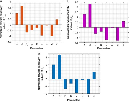In Figure 2(a–c), we plot the normalized forward sensitivity indices to each parameter involved in the expressions of ${\mathcal{R}}_{\mathrm{a}\mathrm{v}}$, ${\text{β}}_{1_c}$ and ${\varphi }_c$, respectively. From these figures, it may be noted that the values of ${\mathcal{R}}_{\mathrm{a}\mathrm{v}}$, ${\text{β}}_{1_c}$ and ${\varphi }_c$ increase with increase in the values of the parameters Λ, β and δ as these parameters have positive indices with ${\mathcal{R}}_{\mathrm{a}\mathrm{v}}$, ${\text{β}}_{1_c}$ and ${\varphi }_c$. On the other hand, from Figure 2(a), it is evident that the parameters ${\text{β}}_1$, ϕ, K, ν, α and d possess negative indices with ${\mathcal{R}}_{\mathrm{a}\mathrm{v}}$. In Figure 2(b), the parameters having negative indices with ${\text{β}}_{1_c}$ are ϕ, K, ν, α and d whereas from Figure 2(c), it is easy to note that the parameters having negative indices with ${\varphi }_c$ are ${\text{β}}_1$, K, ν, α and d. The increment in parameters having negative indices result in decline in the values of ${\mathcal{R}}_{\mathrm{a}\mathrm{v}}$, ${\text{β}}_{1_c}$ and ${\varphi }_c$. From Figure 2(a–c), we observe that the parameter β is most sensitive for ${\mathcal{R}}_{\mathrm{a}\mathrm{v}}$, ${\text{β}}_{1_c}$ and ${\varphi }_c$. The sensitivity indices give that increase in the parameter β by 1% will result in 1.67%, 2.29% and 3.33% increase in the values of ${\mathcal{R}}_{\mathrm{a}\mathrm{v}}$, ${\text{β}}_{1_c}$ and ${\varphi }_c$, respectively. Note that our objective is to prefer the lower values of ${\mathcal{R}}_{\mathrm{a}\mathrm{v}}$, ${\text{β}}_{1_c}$ and ${\varphi }_c$ as they enhance the possibility of disease eradication. Therefore, increment in parameters β, Λ and δ must be preventable by all means, while increase in ${\text{β}}_1$, ϕ, K, ν, α, d should instead be favoured. Thus, for disease eradication, any external measures by government officials and policy makers must focus to prevent an increase in the parameters having positive indices with basic reproduction number (${\mathcal{R}}_{\mathrm{a}\mathrm{v}}$ ), critical threshold of efficacy of budget allocation to reduce the contact rate via propagating awareness (${\text{β}}_{1_c}$) and critical threshold of vaccination rate among susceptible individuals in the presence of budget allocation (${\varphi }_c$) whereas the parameter having negative indices should be stimulated by all means.

Figure 2. Normalized forward sensitivity indices of (a) ${\mathcal{R}}_{\mathrm{a}\mathrm{v}}$, (b) ${\text{β}}_{1_c}$ and (c) ${\varphi }_c$ with respect to model parameters. Parameters are at the same values as in Table 1 except $\alpha =0.02$.

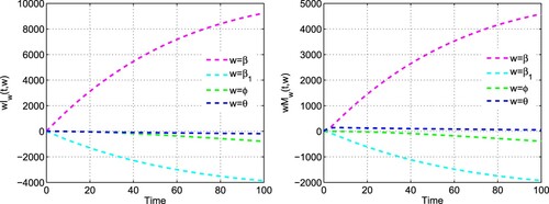
Now, following the method of [5, 39], we determine semi-relative sensitivity solutions for the infective population and budget allocation with respect to some important parameters: β, ${\text{β}}_1$, ϕ and θ. Let us denote $X_w$ as the sensitivity function of a state variable X with respect to a parameter w, i.e.${\displaystyle X_w(t,w)=\frac{\mathrm{\partial }}{\mathrm{\partial }w}X(t,w).}$ The semi-relative sensitivity solutions ${\displaystyle \left(i.e.,w{X}_w\right(t,w\left)\right),}$ determine the change that doubling of a parameter yields in the value of a state variable. We fix the parameters at the same values as in Table 1, and plot the semi-relative sensitivity solutions for the infective population and budget allocation in Figure 3. It is apparent from the figures that doubling the contact rate in the absence of budget allocation β, increases the number of infected individuals by 9227 persons and amount of budget allocation by 4587 dollars in 100 days. There is decline in infective cases by 3870 persons and amount of budget regarding preventive measures by 1924 dollars on doubling the efficacy of budget allocation to reduce the contact rate via propagating awareness ${\text{β}}_1$ in 100 days. A doubling of the vaccination rate in the presence of budget, ϕ, decreases the infective cases by 793 persons and amount of budget for vaccination and awareness by 388.3 dollars in 100 days. The number of infectives decreases by 194 persons whereas budget allocation increases by 56.29 dollars in 100 days when doubling the per-capita growth rate of budget allocation θ. It is clear that out of these four parameters, β has the maximum positive effect whereas ${\text{β}}_1$ has the maximum negative effect on the number of infective cases. Thus, for disease eradication, the contact rate of susceptibles with infectives should be reduced while the amount of budget on broadcasting informations through different modes of social media like Twitter, Facebook and WhatsApp must be increased by the government officials.

Figure 3. Semi-relative sensitivity solutions for infective population (I) and budget allocation (M) with respect to the parameters β, ${\text{β}}_1$, ϕ and θ. Parameters are at the same values as in Table 1.

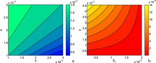
6.2. Impacts of key parameters on ${\mathcal{R}}_{\mathrm{a}\mathrm{v}}$, ${\text{β}}_{1_c}$ and ${\varphi }_c$

To explore the impacts of three important control parameters – the efficacy of budget allocation to reduce the contact rate (${\text{β}}_1$), the vaccination rate among susceptible individuals in the presence of budget allocation (ϕ) and carrying capacity of budget allocation (K), on the epidemic threshold (${\mathcal{R}}_{\mathrm{a}\mathrm{v}}$ ), we have drawn contour plots in Figure 4(a–b). From these contour plots, it is evident that for small values of ${\text{β}}_1$, ϕ and K, the value of basic reproduction number (${\mathcal{R}}_{\mathrm{a}\mathrm{v}}$) is higher; however upon increasing the values of these control parameters above a threshold value, the epidemic threshold (${\mathcal{R}}_{\mathrm{a}\mathrm{v}}$) can be drawn below unity. Thus, using these figures, the requisite value of these parameters for attaining disease-free equilibrium can be computed. It is inferred that the epidemic threshold can be driven to disease free zone in the presence of allocation of budget for vaccination and awareness programs and thus can significantly reduce the burden of disease. Next, we plot the critical values ${\text{β}}_{1_c}$ and ${\varphi }_c$, Figure 5. From these contour plots, it is inferred that the values of ${\text{β}}_{1_c}$ and ${\varphi }_c$ can be reduced with increase in the values of ϕ and ${\text{β}}_1$, respectively, whereas increase in the parameter δ leads to rise in the values of ${\text{β}}_{1_c}$ and ${\varphi }_c$.

Figure 4. Contour plots of the basic reproduction number (${\mathcal{R}}_{\mathrm{a}\mathrm{v}}$) with respect to (a) ${\text{β}}_1$ and K, and (b) ϕ and K. The dashed blue line represents ${\mathcal{R}}_{\mathrm{a}\mathrm{v}}=1$. Rest of the parameters are at the same values as in Table 1.

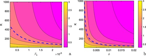
Figure 5. Contour plots of (a) ${\text{β}}_{1_c}$ with respect to ϕ and δ, and (b) ${\varphi }_c$ with respect to ${\text{β}}_1$ and δ. Rest of the parameters are at the same values as in Table 1.

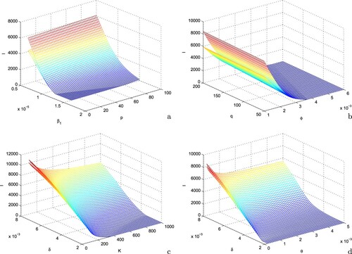
6.3. Impacts of important parameters on disease control

In Figure 6, we plot the infective population by varying two parameters at a time viz. $({\text{β}}_1,p)$, $(\varphi ,q)$, $(K,\delta )$ and $(\theta ,\delta )$. In the figures, surfaces represent the equilibrium level of infective population or the maximum and minimum values of infective population when they oscillate. From Figure 6(a,b), it is inferred that there is rapid decline in infective cases with the increase in efficacy of budget allocation to reduce the contact rate via propagating awareness and vaccination rate among susceptible individuals in the presence of budget whereas infective population increases with the increase in the values of p and q. This is because the contact rate between susceptible and infected individuals increases and vaccination rate in the presence of budget decreases with the increase in the values of these parameters. From Figure 6(c,d), it can be easily seen that the infective population increases very fast due to ineffectiveness of vaccine which can be prevented via continuous propagation of vaccination coverage. On the other hand, there is rapid decline in infective cases with increase in the per-capita growth rate of budget allocation due to increase in infected individuals and carrying capacity of budget allocation. Thus, to suppress the burden of disease among the community, budget allocation must be increased for vaccination and awareness programs.

Figure 6. Surface plots of infective population (I) with respect to (a) ${\text{β}}_1$ and p, (b) ϕ and q, (c) K and δ, and (d) θ and δ. Rest of the parameters are at the same values as in Table 1.

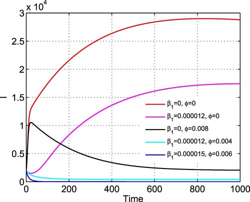
In Figure 7, we plot the number of infected individuals with respect to time for different values of ${\text{β}}_1$ and ϕ, keeping the rest of the parameters at the same values as in Table 1. First, we choose ${\text{β}}_1=\varphi =0$, i.e.when individuals do not take any protective measures to avoid their contacts with infected individuals and there is no vaccination coverage in the region; we find that the equilibrium number of infectives is very high in such case. Next, we assume that the individuals started to adopt precautionary measures to avoid their contacts with infected individuals in the presence of budget allocation to warn people but there is no vaccination coverage in the region. In this case, the number of infectives is found to attain a lower equilibrium level than in the previous case. A substantial decrease in infected population is noted if there is continuous growth in vaccination coverage in the presence of budget despite of the fact that the efficacy of budget allocation to reduce the contact rate via propagating awareness is zero. Further, we consider that the individuals effectively adopt the protective measures to avoid their contact with infected individuals in the presence of awareness and there is continuous growth in vaccination coverage in the presence of budget allocation; due to this combined effects of vaccination and awareness among the individuals, the equilibrium number of infectives decreases to a much lower value. Finally, we see that the equilibrium level of infective becomes zero if there is continuous augmentation in vaccination coverage at higher rate and/or the individuals effectively adopt all precautionary measures to avoid their contacts with infectives. Thus, the combined effects of vaccination coverage and awareness among the individuals regarding protective measures in the presence of budget allocation have potential to reduce the equilibrium number of infectives and can drive the system to disease-free zone.

Figure 7. Effects of vaccination and awareness on the equilibrium level of infective population. Parameters are at the same values as in Table 1.

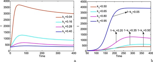
In Figure 8(a–b), we have plotted the variation of infected population $I\left(t\right)$ with respect to time t for different values of $k_1$ (when conditions ${\mathcal{H}}_1>{\mathcal{H}}_2(k_1<k_{1_c}=0.4393)$ and ${\mathcal{H}}_1<{\mathcal{H}}_2(k_1>k_{1_c})$ are satisfied) to determine the effect of the fraction of budget allocation used to warn people via propagating awareness and for vaccination coverage. From these figures, it is apparent that the equilibrium number of infected individuals decreases with the increase in fractional constant of budget allocation used to warn people via propagating awareness up to a threshold value i.e. $k_1<k_{1_c}=0.4393$ (when condition ${\mathcal{H}}_1>{\mathcal{H}}_2$ is satisfied). In this case, fraction of budget allocation used to warn people via propagating awareness is responsible to reduce the equilibrium number of infected individuals. However, further increase in values of $k_1$ above a threshold value ($k_1>k_{1_c}$), fraction of budget allocation used for vaccination coverage (i.e. $1-k_1$) is responsible to reduce the equilibrium number of infected individuals. For the parameter values in Table 1, it is observed that up to $43.93\mathrm{\%}$ of budget used for awareness and the remaining $56.07\mathrm{\%}$ of budget used for vaccination is beneficial to reduce the disease prevalence.

Figure 8. Variation of infected population $I\left(t\right)$ with respect to time t for different values of $k_1$: (a) for ${\mathcal{H}}_1>{\mathcal{H}}_2$ i.e. $k_1<k_{1_c}=0.4393$ and (b) for ${\mathcal{H}}_1<{\mathcal{H}}_2$ i.e. $k_1>k_{1_c}$. Rest of the parameters are at the same values as in Table 1.

In order to manifest the direction of bifurcation at the epidemic threshold ${\mathcal{R}}_{\mathrm{a}\mathrm{v}}=1$, we plot the equilibrium number of infectives with respect to ${\mathcal{R}}_{\mathrm{a}\mathrm{v}}$ by taking β as a function of ${\mathcal{R}}_{\mathrm{a}\mathrm{v}}$, Figure 9. We observe that for small values of β ($\text{β}<{\text{β}}^{\ast }=0.0000224$), the value of ${\mathcal{R}}_{\mathrm{a}\mathrm{v}}$ is less than unity and in this case, only the disease-free equilibrium is feasible and locally asymptotically stable. However, on increasing the values of β above the threshold value ($\text{β}>{\text{β}}^{\ast }$), the value of ${\mathcal{R}}_{\mathrm{a}\mathrm{v}}$ crosses unity, and we find that the interior equilibrium $E^{\ast }$ becomes feasible and locally asymptotically stable whereas the disease-free equilibrium becomes unstable. This implies that the disease can persists (or dies out) in the system whenever ${\mathcal{R}}_{\mathrm{a}\mathrm{v}}>1$ (or ${\mathcal{R}}_{\mathrm{a}\mathrm{v}}<1$ ). 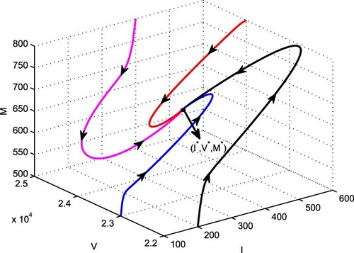Now, we see the global stability of interior equilibrium $E^{\ast }$ in I−V −M space, Figure 10. From this figure, it is apparent that all the solution trajectories in I−V −M space are approaching towards the point $(I^{\ast },V^{\ast },M^{\ast })$ inside the region of attraction Ω. Using this approach, the global asymptotic stability of the interior equilibrium $E^{\ast }$ in other spaces can also be shown. Thus, the statement of the Theorem 3.3 is numerically verified. The global stability of interior equilibrium shows that disease persists in the population when the vaccination rate in the presence of budget and efficacy of budget allocation to reduce the contact rate via propagating awareness are not strong enough.

Figure 9. Forward bifurcation diagram of system (2(2) $\begin{array}{rl}\frac{\mathrm{d}I}{\mathrm{d}t}& =\left(\text{β}-{\text{β}}_1\frac{k_{1}M}{p+k_{1}M}\right)(N-I-V)I-(\nu +\alpha +d)I,\\ \frac{\mathrm{d}V}{\mathrm{d}t}& =\varphi \frac{(1-k_1)M}{q+(1-k_1)M}(N-I-V)-(\delta +d)V,\\ \frac{\mathrm{d}N}{\mathrm{d}t}& =\mathrm{\Lambda }-\mathrm{d}N-\alpha I,\\ \frac{\mathrm{d}M}{\mathrm{d}t}& =rM\left(1-\frac{M}{K}\right)+\theta IM.\end{array}$(2) ). Parameters are at the same values as in Table 1. Blue colour denotes stable disease-free equilibrium ($E_3$), red colour represents unstable disease-free equilibrium ($E_3$) and magenta colour stands for stable interior equilibrium ($E^{\ast }$).

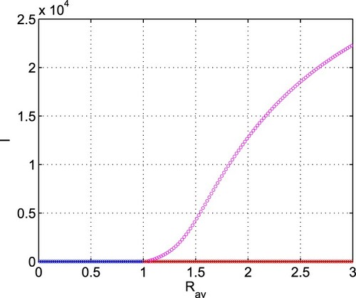
Figure 10. Global stability of the equilibrium $E^{\ast }$ in I−V −M space. Parameters are at the same values as in Table 1.

6.4. Existence of Hopf-bifurcation

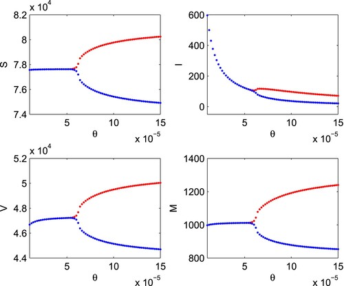
In order to examine the existence of Hopf-bifurcation and the stability of bifurcating periodic solutions, we choose the following set of parameter values: (24) $\begin{array}{rl}& \mathrm{\Lambda }=5,\text{β}=0.0000030,{\text{β}}_1=0.0000018,k_1=0.2,p=2000,\varphi =0.02,q=2500,\\ & \delta =0.008,\nu =0.22,\alpha =0.00001,d=0.00004,r=0.006,K=500.\end{array}$(24) We draw the bifurcation diagram of system (1(1) $\begin{array}{rl}\frac{\mathrm{d}S}{\mathrm{d}t}& =\mathrm{\Lambda }-\left(\text{β}-{\text{β}}_1\frac{k_{1}M}{p+k_{1}M}\right)SI-\varphi \frac{(1-k_1)M}{q+(1-k_1)M}S+\nu I+\delta V-\mathrm{d}S,\\ \frac{\mathrm{d}I}{\mathrm{d}t}& =\left(\text{β}-{\text{β}}_1\frac{k_{1}M}{p+k_{1}M}\right)SI-(\nu +\alpha +d)I,\\ \frac{\mathrm{d}V}{\mathrm{d}t}& =\varphi \frac{(1-k_1)M}{q+(1-k_1)M}S-(\delta +d)V,\\ \frac{\mathrm{d}M}{\mathrm{d}t}& =rM\left(1-\frac{M}{K}\right)+\theta IM.\end{array}$(1) ) with respect to the per-capita growth rate of budget allocation due to increase in infected individuals (θ), Figure 11. From the figure, it is apparent that for small values of θ, all the variables settle down to their equilibrium values while an increase in the value of θ after a threshold value, periodic oscillations arise and the interior equilibrium changes its stability from stable to unstable state. The critical value of θ at which change in stability occurs is found to be ${\theta }_c=0.00005953$. It is clear from the figure that the interior equilibrium is stable for $\theta <{\theta }_c$ whereas loss of stability occurs for $\theta >{\theta }_c$ and the interior equilibrium becomes unstable. Thus, system (1(1) $\begin{array}{rl}\frac{\mathrm{d}S}{\mathrm{d}t}& =\mathrm{\Lambda }-\left(\text{β}-{\text{β}}_1\frac{k_{1}M}{p+k_{1}M}\right)SI-\varphi \frac{(1-k_1)M}{q+(1-k_1)M}S+\nu I+\delta V-\mathrm{d}S,\\ \frac{\mathrm{d}I}{\mathrm{d}t}& =\left(\text{β}-{\text{β}}_1\frac{k_{1}M}{p+k_{1}M}\right)SI-(\nu +\alpha +d)I,\\ \frac{\mathrm{d}V}{\mathrm{d}t}& =\varphi \frac{(1-k_1)M}{q+(1-k_1)M}S-(\delta +d)V,\\ \frac{\mathrm{d}M}{\mathrm{d}t}& =rM\left(1-\frac{M}{K}\right)+\theta IM.\end{array}$(1) ) undergoes Hopf-bifurcation around the interior equilibrium at $\theta ={\theta }_c$. Further, the sign of ${\mu }_2$, ${\text{β}}_2$, $T_2$ at $\theta ={\theta }_c$ are simulated to be $4.08\times {10}^{-12}$, $-1.76\times {10}^{-11}$, and $9.24\times {10}^{-10}$, respectively. Therefore, using Theorem 3.5, we can say that Hopf-bifurcation is supercritical and bifurcating periodic solutions exist for $\theta >{\theta }_c$; the bifurcating periodic solutions are stable and period increases.

Figure 11. Bifurcation diagram of system (1(1) $\begin{array}{rl}\frac{\mathrm{d}S}{\mathrm{d}t}& =\mathrm{\Lambda }-\left(\text{β}-{\text{β}}_1\frac{k_{1}M}{p+k_{1}M}\right)SI-\varphi \frac{(1-k_1)M}{q+(1-k_1)M}S+\nu I+\delta V-\mathrm{d}S,\\ \frac{\mathrm{d}I}{\mathrm{d}t}& =\left(\text{β}-{\text{β}}_1\frac{k_{1}M}{p+k_{1}M}\right)SI-(\nu +\alpha +d)I,\\ \frac{\mathrm{d}V}{\mathrm{d}t}& =\varphi \frac{(1-k_1)M}{q+(1-k_1)M}S-(\delta +d)V,\\ \frac{\mathrm{d}M}{\mathrm{d}t}& =rM\left(1-\frac{M}{K}\right)+\theta IM.\end{array}$(1) ) with respect to θ. Rest of the parameters are at the same values as in (24(24) $\begin{array}{rl}& \mathrm{\Lambda }=5,\text{β}=0.0000030,{\text{β}}_1=0.0000018,k_1=0.2,p=2000,\varphi =0.02,q=2500,\\ & \delta =0.008,\nu =0.22,\alpha =0.00001,d=0.00004,r=0.006,K=500.\end{array}$(24) ). Here, red colour represents the upper limit of oscillation cycle and blue colour represents the lower limit of oscillation cycle.

6.5. Impact of delay in budget allocation

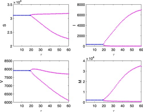
We choose the following set of parameter values for the simulation results of system (16(16) $\begin{array}{rl}\frac{\mathrm{d}I}{\mathrm{d}t}& =\left(\text{β}-{\text{β}}_1\frac{k_{1}M}{p+k_{1}M}\right)(N-I-V)I-(\nu +\alpha +d)I,\\ \frac{\mathrm{d}V}{\mathrm{d}t}& =\frac{\varphi (1-k_1)M}{q+(1-k_1)M}(N-I-V)-(\delta +d)V,\\ \frac{\mathrm{d}N}{\mathrm{d}t}& =\mathrm{\Lambda }-\mathrm{d}N-\alpha I,\\ \frac{\mathrm{d}M}{\mathrm{d}t}& =rM\left(1-\frac{M}{K}\right)+\theta I(t-\tau )M.\end{array}$(16) ): (25) $\begin{array}{rl}& \mathrm{\Lambda }=400,\text{β}=0.000048,{\text{β}}_1=0.000040,k_1=0.4,p=60,\varphi =0.005,q=120,\\ & \delta =0.008,\nu =0.3,\alpha =0.02,d=0.01,r=0.005,K=500,\theta =\mathrm{0.00005.}\end{array}$(25) For the set of parameter values given in (25(25) $\begin{array}{rl}& \mathrm{\Lambda }=400,\text{β}=0.000048,{\text{β}}_1=0.000040,k_1=0.4,p=60,\varphi =0.005,q=120,\\ & \delta =0.008,\nu =0.3,\alpha =0.02,d=0.01,r=0.005,K=500,\theta =\mathrm{0.00005.}\end{array}$(25) ), it is observed that Equation  (22(22) $H\left(\eta \right)\equiv {\eta }^4+C_1{\eta }^3+C_2{\eta }^2+C_3\eta +C_4=0,$(22) ) has exactly one positive real root, i.e.transcendental equation (19(19) $D(\zeta ,\tau )={\zeta }^4+p_1{\zeta }^3+p_2{\zeta }^2+p_3\zeta +p_4+(q_0{\zeta }^2+q_1\zeta +q_2)e^{-\zeta \tau }=0,$(19) ) has a pair of purely imaginary roots and the critical value of time delay is obtained as ${\tau }_0=19.80$ days at which the system's behaviour changes drastically. Using Theorem 5.3, we can say that the equilibrium $E^{\ast }$ is stable for $\tau \in [0,{\tau }_0)$ and unstable for $\tau >{\tau }_0$. To see the impact of time delay in per-capita growth rate of budget allocation, we draw the bifurcation diagram of system (16(16) $\begin{array}{rl}\frac{\mathrm{d}I}{\mathrm{d}t}& =\left(\text{β}-{\text{β}}_1\frac{k_{1}M}{p+k_{1}M}\right)(N-I-V)I-(\nu +\alpha +d)I,\\ \frac{\mathrm{d}V}{\mathrm{d}t}& =\frac{\varphi (1-k_1)M}{q+(1-k_1)M}(N-I-V)-(\delta +d)V,\\ \frac{\mathrm{d}N}{\mathrm{d}t}& =\mathrm{\Lambda }-\mathrm{d}N-\alpha I,\\ \frac{\mathrm{d}M}{\mathrm{d}t}& =rM\left(1-\frac{M}{K}\right)+\theta I(t-\tau )M.\end{array}$(16) ) by taking time delay τ as a bifurcation parameter, Figure 12. The figure shows that all the variables settle down to their equilibrium values for $\tau \in [0,{\tau }_0)$ while for $\tau >{\tau }_0$, the system exhibits unstable dynamics through limit cycle oscillations with increasing amplitude.

Figure 12. Bifurcation diagram of system (16(16) $\begin{array}{rl}\frac{\mathrm{d}I}{\mathrm{d}t}& =\left(\text{β}-{\text{β}}_1\frac{k_{1}M}{p+k_{1}M}\right)(N-I-V)I-(\nu +\alpha +d)I,\\ \frac{\mathrm{d}V}{\mathrm{d}t}& =\frac{\varphi (1-k_1)M}{q+(1-k_1)M}(N-I-V)-(\delta +d)V,\\ \frac{\mathrm{d}N}{\mathrm{d}t}& =\mathrm{\Lambda }-\mathrm{d}N-\alpha I,\\ \frac{\mathrm{d}M}{\mathrm{d}t}& =rM\left(1-\frac{M}{K}\right)+\theta I(t-\tau )M.\end{array}$(16) ) with respect to τ. Rest of the parameters are at the same values as in (25(25) $\begin{array}{rl}& \mathrm{\Lambda }=400,\text{β}=0.000048,{\text{β}}_1=0.000040,k_1=0.4,p=60,\varphi =0.005,q=120,\\ & \delta =0.008,\nu =0.3,\alpha =0.02,d=0.01,r=0.005,K=500,\theta =\mathrm{0.00005.}\end{array}$(25) ). Here, blue colour represents stability of the interior equilibrium and magenta colour corresponds to instability of the interior equilibrium.

Further, we observed that for ${\text{β}}_1=0.000034$, p = 500, $\varphi =0.05$, q = 800 and $\delta =0.08$, and rest of the parameters are at the same values as in (25(25) $\begin{array}{rl}& \mathrm{\Lambda }=400,\text{β}=0.000048,{\text{β}}_1=0.000040,k_1=0.4,p=60,\varphi =0.005,q=120,\\ & \delta =0.008,\nu =0.3,\alpha =0.02,d=0.01,r=0.005,K=500,\theta =\mathrm{0.00005.}\end{array}$(25) ), Equation (22(22) $H\left(\eta \right)\equiv {\eta }^4+C_1{\eta }^3+C_2{\eta }^2+C_3\eta +C_4=0,$(22) ) has two positive real roots ${\eta }^{+}=0.00146$ and ${\eta }^{-}=0.000394$ (where ${\eta }^{+}>{\eta }^{-}$) i.e. the characteristic equation (19(19) $D(\zeta ,\tau )={\zeta }^4+p_1{\zeta }^3+p_2{\zeta }^2+p_3\zeta +p_4+(q_0{\zeta }^2+q_1\zeta +q_2)e^{-\zeta \tau }=0,$(19) ) has two pairs of purely imaginary roots $\pm {\omega }_{\pm }$. For these positive values of ${\omega }_{\pm }$ from equation (23(23) $\begin{array}{rl}{\tau }_k^{\pm }& =\frac{(2k+1)\pi }{{\omega }_{\pm }}\\ & +\frac{1}{{\omega }_{\pm }}{\tan }^{-1}\left[\frac{({\omega }_{\pm }^4-p_2{\omega }_{\pm }^2+p_4)q_1{\omega }_{\pm }+(p_1{\omega }_{\pm }^3-p_3{\omega }_{\pm })(q_2-q_0{\omega }_{\pm }^2)}{({\omega }_{\pm }^4-p_2{\omega }_{\pm }^2+p_4)(q_2-q_0{\omega }_{\pm }^2)-q_1{\omega }_{\pm }(p_1{\omega }_{\pm }^3-p_3{\omega }_{\pm })}\right],\end{array}$(23) ), we found the positive values of ${\tau }_k^{\pm }$ $(k=0,1,2,3,\dots )$ as given in Table 2. Using Theorem 5.5, we can say that for the above set of parameter values, the interior equilibrium $E^{\ast }$ is stable for $\tau \in [0,61)\cup (156,225)$ and unstable for $\tau \in (61,156)\cup (225,472)$.

Table 2. Critical values of τ.

${\tau }_0^{+}$=61 days	${\tau }_1^{+}$=225 days	${\tau }_2^{+}$=390 days	${\tau }_3^{+}$=554 days	···
${\tau }_0^{-}$=156 days	${\tau }_1^{-}$=472 days	${\tau }_2^{-}$=788 days	${\tau }_3^{-}$=1105 days	···

We pick values of time delay from different intervals and plot the infective population (it is noted that other variables of the system (16(16) $\begin{array}{rl}\frac{\mathrm{d}I}{\mathrm{d}t}& =\left(\text{β}-{\text{β}}_1\frac{k_{1}M}{p+k_{1}M}\right)(N-I-V)I-(\nu +\alpha +d)I,\\ \frac{\mathrm{d}V}{\mathrm{d}t}& =\frac{\varphi (1-k_1)M}{q+(1-k_1)M}(N-I-V)-(\delta +d)V,\\ \frac{\mathrm{d}N}{\mathrm{d}t}& =\mathrm{\Lambda }-\mathrm{d}N-\alpha I,\\ \frac{\mathrm{d}M}{\mathrm{d}t}& =rM\left(1-\frac{M}{K}\right)+\theta I(t-\tau )M.\end{array}$(16) ) have similar behaviours), Figure 13. From Figure 13(a), it is observed that for $\tau =30\in [0,61)$, the infected individuals settle down to their equilibrium value, showing the stable dynamics of system (16(16) $\begin{array}{rl}\frac{\mathrm{d}I}{\mathrm{d}t}& =\left(\text{β}-{\text{β}}_1\frac{k_{1}M}{p+k_{1}M}\right)(N-I-V)I-(\nu +\alpha +d)I,\\ \frac{\mathrm{d}V}{\mathrm{d}t}& =\frac{\varphi (1-k_1)M}{q+(1-k_1)M}(N-I-V)-(\delta +d)V,\\ \frac{\mathrm{d}N}{\mathrm{d}t}& =\mathrm{\Lambda }-\mathrm{d}N-\alpha I,\\ \frac{\mathrm{d}M}{\mathrm{d}t}& =rM\left(1-\frac{M}{K}\right)+\theta I(t-\tau )M.\end{array}$(16) ). Further increase in the value of time delay $\tau =100\in (61,156)$ leads to limit cycle oscillations in the infected individuals with increasing amplitude, i.e. the interior equilibrium $E^{\ast }$ shows unstable dynamics (see Figure 13(b)). From Figure 13(c), it is inferred that for $\tau =180\in (156,225)$, the dynamics of system is again stable focus. Furthermore, we see the dynamical behaviour of the system at higher values of time delay, at $\tau =400$ days, the system enters into chaotic regime, Figure 13(d). The occurrence of chaotic oscillation may be explained through incommensurate limit cycle, i.e. the frequency of the first type of oscillation is not multiple of the frequency of the second type of oscillation [21, 22]. Thus, the interior equilibrium $E^{\ast }$ of system (16(16) $\begin{array}{rl}\frac{\mathrm{d}I}{\mathrm{d}t}& =\left(\text{β}-{\text{β}}_1\frac{k_{1}M}{p+k_{1}M}\right)(N-I-V)I-(\nu +\alpha +d)I,\\ \frac{\mathrm{d}V}{\mathrm{d}t}& =\frac{\varphi (1-k_1)M}{q+(1-k_1)M}(N-I-V)-(\delta +d)V,\\ \frac{\mathrm{d}N}{\mathrm{d}t}& =\mathrm{\Lambda }-\mathrm{d}N-\alpha I,\\ \frac{\mathrm{d}M}{\mathrm{d}t}& =rM\left(1-\frac{M}{K}\right)+\theta I(t-\tau )M.\end{array}$(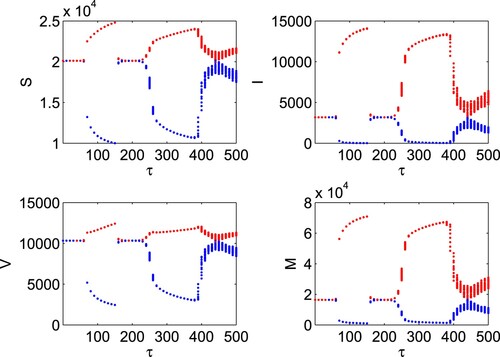16) ) switches from stable to unstable to stable state and eventually system enters into chaotic regime at very high value of time delay. For a better demonstration of the effect of time delay in per-capita growth rate of budget allocation, we draw bifurcation diagram of system (16(16) $\begin{array}{rl}\frac{\mathrm{d}I}{\mathrm{d}t}& =\left(\text{β}-{\text{β}}_1\frac{k_{1}M}{p+k_{1}M}\right)(N-I-V)I-(\nu +\alpha +d)I,\\ \frac{\mathrm{d}V}{\mathrm{d}t}& =\frac{\varphi (1-k_1)M}{q+(1-k_1)M}(N-I-V)-(\delta +d)V,\\ \frac{\mathrm{d}N}{\mathrm{d}t}& =\mathrm{\Lambda }-\mathrm{d}N-\alpha I,\\ \frac{\mathrm{d}M}{\mathrm{d}t}& =rM\left(1-\frac{M}{K}\right)+\theta I(t-\tau )M.\end{array}$(16) ) by varying the delay parameter τ in the interval $[0,500]$, Figure 14. From the figure, it is inferred that for $\tau \in [0,61)\cup (156,225)$, all the dynamical variables attain their equilibrium values, i.e. interior equilibrium shows stable dynamics and for $\tau \in (61,156)\cup (225,472)$, all the dynamical variables show oscillatory behaviour whose maximum and minimum values are apparent from the figure, i.e. interior equilibrium shows unstable dynamics and Hopf-bifurcation occurs at $\tau =61,156,225$. Moreover, at very higher values of time delay $\tau \ge 400$ days, the system (16(16) $\begin{array}{rl}\frac{\mathrm{d}I}{\mathrm{d}t}& =\left(\text{β}-{\text{β}}_1\frac{k_{1}M}{p+k_{1}M}\right)(N-I-V)I-(\nu +\alpha +d)I,\\ \frac{\mathrm{d}V}{\mathrm{d}t}& =\frac{\varphi (1-k_1)M}{q+(1-k_1)M}(N-I-V)-(\delta +d)V,\\ \frac{\mathrm{d}N}{\mathrm{d}t}& =\mathrm{\Lambda }-\mathrm{d}N-\alpha I,\\ \frac{\mathrm{d}M}{\mathrm{d}t}& =rM\left(1-\frac{M}{K}\right)+\theta I(t-\tau )M.\end{array}$(16) ) enters into chaotic regime. Thus, the dynamics of system (16(16) $\begin{array}{rl}\frac{\mathrm{d}I}{\mathrm{d}t}& =\left(\text{β}-{\text{β}}_1\frac{k_{1}M}{p+k_{1}M}\right)(N-I-V)I-(\nu +\alpha +d)I,\\ \frac{\mathrm{d}V}{\mathrm{d}t}& =\frac{\varphi (1-k_1)M}{q+(1-k_1)M}(N-I-V)-(\delta +d)V,\\ \frac{\mathrm{d}N}{\mathrm{d}t}& =\mathrm{\Lambda }-\mathrm{d}N-\alpha I,\\ \frac{\mathrm{d}M}{\mathrm{d}t}& =rM\left(1-\frac{M}{K}\right)+\theta I(t-\tau )M.\end{array}$(16) ) changes from stable to limit cycle oscillations to stable to limit cycle oscillations to chaos on increasing the values of time delay.

Figure 13. Time series of system (16(16) $\begin{array}{rl}\frac{\mathrm{d}I}{\mathrm{d}t}& =\left(\text{β}-{\text{β}}_1\frac{k_{1}M}{p+k_{1}M}\right)(N-I-V)I-(\nu +\alpha +d)I,\\ \frac{\mathrm{d}V}{\mathrm{d}t}& =\frac{\varphi (1-k_1)M}{q+(1-k_1)M}(N-I-V)-(\delta +d)V,\\ \frac{\mathrm{d}N}{\mathrm{d}t}& =\mathrm{\Lambda }-\mathrm{d}N-\alpha I,\\ \frac{\mathrm{d}M}{\mathrm{d}t}& =rM\left(1-\frac{M}{K}\right)+\theta I(t-\tau )M.\end{array}$(16) ) for different values of τ. Systems shows (a) stable focus at $\tau =30$, (b) limit cycle oscillations at $\tau =100$, (c) stable focus at $\tau =180$ and (d) chaotic dynamics at $\tau =400$. Rest of the parameters are at the same values as in (25(25) $\begin{array}{rl}& \mathrm{\Lambda }=400,\text{β}=0.000048,{\text{β}}_1=0.000040,k_1=0.4,p=60,\varphi =0.005,q=120,\\ & \delta =0.008,\nu =0.3,\alpha =0.02,d=0.01,r=0.005,K=500,\theta =\mathrm{0.00005.}\end{array}$(25) ) except ${\text{β}}_1=0.000034$, p = 500, q = 800, $\varphi =0.05$, $\delta =0.08$.

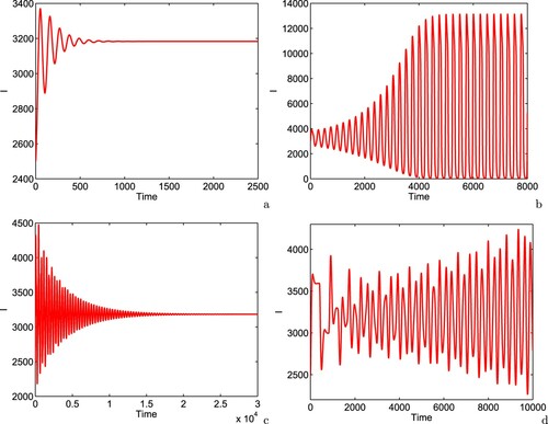
Figure 14. Bifurcation diagram of system (16(16) $\begin{array}{rl}\frac{\mathrm{d}I}{\mathrm{d}t}& =\left(\text{β}-{\text{β}}_1\frac{k_{1}M}{p+k_{1}M}\right)(N-I-V)I-(\nu +\alpha +d)I,\\ \frac{\mathrm{d}V}{\mathrm{d}t}& =\frac{\varphi (1-k_1)M}{q+(1-k_1)M}(N-I-V)-(\delta +d)V,\\ \frac{\mathrm{d}N}{\mathrm{d}t}& =\mathrm{\Lambda }-\mathrm{d}N-\alpha I,\\ \frac{\mathrm{d}M}{\mathrm{d}t}& =rM\left(1-\frac{M}{K}\right)+\theta I(t-\tau )M.\end{array}$(16) ) with respect to τ. Rest of the parameters are at the same values as in (25(25) $\begin{array}{rl}& \mathrm{\Lambda }=400,\text{β}=0.000048,{\text{β}}_1=0.000040,k_1=0.4,p=60,\varphi =0.005,q=120,\\ & \delta =0.008,\nu =0.3,\alpha =0.02,d=0.01,r=0.005,K=500,\theta =\mathrm{0.00005.}\end{array}$(25) ) except ${\text{β}}_1=0.000034$, p = 500, q = 800, $\varphi =0.05$, $\delta =0.08$. Here, red colour represents the upper limit of oscillation cycle and blue colour represents the lower limit of oscillation cycle.

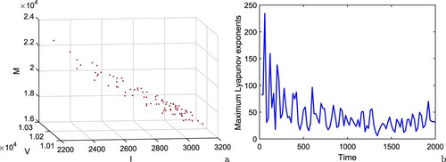
To confirm chaotic nature of the system (16(16) $\begin{array}{rl}\frac{\mathrm{d}I}{\mathrm{d}t}& =\left(\text{β}-{\text{β}}_1\frac{k_{1}M}{p+k_{1}M}\right)(N-I-V)I-(\nu +\alpha +d)I,\\ \frac{\mathrm{d}V}{\mathrm{d}t}& =\frac{\varphi (1-k_1)M}{q+(1-k_1)M}(N-I-V)-(\delta +d)V,\\ \frac{\mathrm{d}N}{\mathrm{d}t}& =\mathrm{\Lambda }-\mathrm{d}N-\alpha I,\\ \frac{\mathrm{d}M}{\mathrm{d}t}& =rM\left(1-\frac{M}{K}\right)+\theta I(t-\tau )M.\end{array}$(16) ), we draw Poincaré map of the system (16(16) $\begin{array}{rl}\frac{\mathrm{d}I}{\mathrm{d}t}& =\left(\text{β}-{\text{β}}_1\frac{k_{1}M}{p+k_{1}M}\right)(N-I-V)I-(\nu +\alpha +d)I,\\ \frac{\mathrm{d}V}{\mathrm{d}t}& =\frac{\varphi (1-k_1)M}{q+(1-k_1)M}(N-I-V)-(\delta +d)V,\\ \frac{\mathrm{d}N}{\mathrm{d}t}& =\mathrm{\Lambda }-\mathrm{d}N-\alpha I,\\ \frac{\mathrm{d}M}{\mathrm{d}t}& =rM\left(1-\frac{M}{K}\right)+\theta I(t-\tau )M.\end{array}$(16) ) in I−V −M space at S = 20000 for $\tau =4000$ days, Figure 15(a). The scattered distribution of the sampling points implies the chaotic behaviour of the system. We also plot maximum Lyapunov exponent of the system (16(16) $\begin{array}{rl}\frac{\mathrm{d}I}{\mathrm{d}t}& =\left(\text{β}-{\text{β}}_1\frac{k_{1}M}{p+k_{1}M}\right)(N-I-V)I-(\nu +\alpha +d)I,\\ \frac{\mathrm{d}V}{\mathrm{d}t}& =\frac{\varphi (1-k_1)M}{q+(1-k_1)M}(N-I-V)-(\delta +d)V,\\ \frac{\mathrm{d}N}{\mathrm{d}t}& =\mathrm{\Lambda }-\mathrm{d}N-\alpha I,\\ \frac{\mathrm{d}M}{\mathrm{d}t}& =rM\left(1-\frac{M}{K}\right)+\theta I(t-\tau )M.\end{array}$(16) ) at $\tau =400$ days by using the algorithm of [42, 53], Figure 15(b). The maximum Lyapunov exponent has been proven to be most useful dynamical diagnostic for chaotic systems. It represents the average exponential rate of convergence/divergence of nearby orbits in the phase space. The idea of calculating its value is to follow two nearby orbits and calculate their average logarithmic rate of separation. Whenever they get too far apart, one of the orbits has to be moved back to the vicinity of the other along the line of separation. If the attractor is chaotic, the maximum Lyapunov exponent is positive; for a bifurcation point, the maximum Lyapunov exponent is zero; the negative values of maximum Lyapunov exponent correspond to a fixed point/periodic attractor. To plot the maximum Lyapunov exponent, the delayed system (16(16) $\begin{array}{rl}\frac{\mathrm{d}I}{\mathrm{d}t}& =\left(\text{β}-{\text{β}}_1\frac{k_{1}M}{p+k_{1}M}\right)(N-I-V)I-(\nu +\alpha +d)I,\\ \frac{\mathrm{d}V}{\mathrm{d}t}& =\frac{\varphi (1-k_1)M}{q+(1-k_1)M}(N-I-V)-(\delta +d)V,\\ \frac{\mathrm{d}N}{\mathrm{d}t}& =\mathrm{\Lambda }-\mathrm{d}N-\alpha I,\\ \frac{\mathrm{d}M}{\mathrm{d}t}& =rM\left(1-\frac{M}{K}\right)+\theta I(t-\tau )M.\end{array}$(16) ) is first simulated, then by considering the time series solutions of each component of the system, the maximum Lyapunov exponent is computed. In Figure 15(b), the positive values of maximum Lyapunov exponent demonstrate the chaotic regime of system (16(16) $\begin{array}{rl}\frac{\mathrm{d}I}{\mathrm{d}t}& =\left(\text{β}-{\text{β}}_1\frac{k_{1}M}{p+k_{1}M}\right)(N-I-V)I-(\nu +\alpha +d)I,\\ \frac{\mathrm{d}V}{\mathrm{d}t}& =\frac{\varphi (1-k_1)M}{q+(1-k_1)M}(N-I-V)-(\delta +d)V,\\ \frac{\mathrm{d}N}{\mathrm{d}t}& =\mathrm{\Lambda }-\mathrm{d}N-\alpha I,\\ \frac{\mathrm{d}M}{\mathrm{d}t}& =rM\left(1-\frac{M}{K}\right)+\theta I(t-\tau )M.\end{array}$(16) ).

Figure 15. (a) Poincaré map of the system (16(16) $\begin{array}{rl}\frac{\mathrm{d}I}{\mathrm{d}t}& =\left(\text{β}-{\text{β}}_1\frac{k_{1}M}{p+k_{1}M}\right)(N-I-V)I-(\nu +\alpha +d)I,\\ \frac{\mathrm{d}V}{\mathrm{d}t}& =\frac{\varphi (1-k_1)M}{q+(1-k_1)M}(N-I-V)-(\delta +d)V,\\ \frac{\mathrm{d}N}{\mathrm{d}t}& =\mathrm{\Lambda }-\mathrm{d}N-\alpha I,\\ \frac{\mathrm{d}M}{\mathrm{d}t}& =rM\left(1-\frac{M}{K}\right)+\theta I(t-\tau )M.\end{array}$(16) ) in I−V −M space at S = 20000 for $\tau =4000$ days, and (b) maximum Lyapunov exponent of the system (16(16) $\begin{array}{rl}\frac{\mathrm{d}I}{\mathrm{d}t}& =\left(\text{β}-{\text{β}}_1\frac{k_{1}M}{p+k_{1}M}\right)(N-I-V)I-(\nu +\alpha +d)I,\\ \frac{\mathrm{d}V}{\mathrm{d}t}& =\frac{\varphi (1-k_1)M}{q+(1-k_1)M}(N-I-V)-(\delta +d)V,\\ \frac{\mathrm{d}N}{\mathrm{d}t}& =\mathrm{\Lambda }-\mathrm{d}N-\alpha I,\\ \frac{\mathrm{d}M}{\mathrm{d}t}& =rM\left(1-\frac{M}{K}\right)+\theta I(t-\tau )M.\end{array}$(16) ) at $\tau =400$ days. Rest of the parameters are at the same values as in (25(25) $\begin{array}{rl}& \mathrm{\Lambda }=400,\text{β}=0.000048,{\text{β}}_1=0.000040,k_1=0.4,p=60,\varphi =0.005,q=120,\\ & \delta =0.008,\nu =0.3,\alpha =0.02,d=0.01,r=0.005,K=500,\theta =\mathrm{0.00005.}\end{array}$(25) ) except ${\text{β}}_1=0.000034$, p = 500, q = 800, $\varphi =0.05$, $\delta =0.08$.

7. Conclusion and discussion

In this paper, we investigated the effects of budget allocation for vaccination and awareness to control the directly transmitted diseases. The model analysis reveals that the increment in budget allocation for vaccination coverage and awareness among the individuals regarding protective measures have potential to reduce the epidemic size and drives the system to disease-free zone. Our sensitivity results suggest that the government officials and policy makers should pay significant attention to allocate funds for vaccination coverage and broadcasting of information regarding protective measures so that individuals adopt all precautionary measures in order to eliminate the burden of disease in the community. Although, the ineffectiveness of vaccine causes longer persistence of disease in the society, budget allocation can maintain active vaccination coverage in the society, and subsequently control the spread of infection. A significant decrease in infective population is noted with the increment in budget allocation.

The model analysis showed that up to 43.93% of budget should be used for awareness and the remaining 56.07% of budget should be used for vaccination to reduce the severity of disease. The simulation results indicate that if the vaccine is not effective, then one should focus on the propagation of awareness programs at higher level for disease eradication. Similarly, if the people are not much aware about the disease, the prevalence of disease can be terminated by raising the efficacy of vaccines. Moreover, the combined effects of vaccination of high quality and the propagation of awareness at higher rate are beneficial to control the spread of disease in the population. Our simulation results showed that the increment in per-capita growth rate of budget allocation due to increase in infected individuals after a threshold value destabilizes the system and periodic oscillations arise through Hopf-bifurcation.

To predict more realistic situation on system dynamics, a discrete time delay is incorporated in per-capita growth rate of budget allocation due to increase in infected individuals. Our findings indicate that continuous and timely allocation of funds regarding preventive measures is beneficial to suppress the burden of disease in the community. However, longer delay in reported cases of infected individuals, i.e. delay in providing funds by government officials and policy makers destabilizes the system and unpredictable behaviour may be observed in the system, which brings challenges to predict and control the epidemic, and have possibility of occurrence of multiple epidemic outbreaks. Previous studies have shown the occurrence of limit cycle oscillations and multiple stability switches due to delay involved in increments of budget allocation [35, 43]. Our study shows an extra and interesting dynamics; chaotic behaviour is observed in the delayed system through incommensurate limit cycle for longer delay in per-capita growth rate of budget allocation due to rise in infected population.

Nowadays, due to emergence of coronavirus pandemic, developing and underdeveloped countries are facing huge economic crisis due to long-term lockdowns and cuts in businesses and other economic activities which resulted in rapid decline in government revenue. To overcome this, government of several countries have started to breakdown and cut in education funds, health-care funds, health infrastructure, medical health facilities etc., in coming days. However, public self-awareness regarding preventive measures such as frequent hand washing, maintaining social distance, having a healthy diet, use of face masks, regularly sanitizing etc., help people to fight against the pandemic together. Thus, the self-induced behavioural changes are vital options if there is delay in implementation of health care policies to fight against the pandemic.

Acknowledgements

The authors thank the associate editor and anonymous reviewers for their valuable comments, which contributed to the improvement in the presentation of the paper.

Disclosure statement

No potential conflict of interest was reported by the author(s).

Appendix 1

The Jacobian matrix of system (2(2) $\begin{array}{rl}\frac{\mathrm{d}I}{\mathrm{d}t}& =\left(\text{β}-{\text{β}}_1\frac{k_{1}M}{p+k_{1}M}\right)(N-I-V)I-(\nu +\alpha +d)I,\\ \frac{\mathrm{d}V}{\mathrm{d}t}& =\varphi \frac{(1-k_1)M}{q+(1-k_1)M}(N-I-V)-(\delta +d)V,\\ \frac{\mathrm{d}N}{\mathrm{d}t}& =\mathrm{\Lambda }-\mathrm{d}N-\alpha I,\\ \frac{\mathrm{d}M}{\mathrm{d}t}& =rM\left(1-\frac{M}{K}\right)+\theta IM.\end{array}$(2) ) is $J=[J_{ij}{]}_{4\times 4}$, whose entries are given by $\begin{array}{rl}& J_{11}=\left(\text{β}-{\text{β}}_1\frac{k_{1}M}{p+k_{1}M}\right)(N-2I-V)-(\nu +\alpha +d),J_{12}=-\left(\text{β}-{\text{β}}_1\frac{k_{1}M}{p+k_{1}M}\right)I,\\ & J_{13}=\left(\text{β}-{\text{β}}_1\frac{k_{1}M}{p+k_{1}M}\right)I,J_{14}=\frac{-{\text{β}}_1{k}_{1}p(N-I-V)I}{(p+k_{1}M{)}^2},J_{21}=-\varphi \frac{(1-k_1)M}{q+(1-k_1)M},\\ & J_{22}=-\left(\varphi \frac{(1-k_1)M}{q+(1-k_1)M}+\delta +d\right),J_{23}=\varphi \frac{(1-k_1)M}{q+(1-k_1)M},J_{24}=\frac{\varphi (1-k_1)q(N-I-V)}{(q+(1-k_1)M{)}^2},\\ & J_{31}=-\alpha ,J_{33}=-d,J_{41}=\theta M,J_{44}=r\left(1-2\frac{M}{K}\right)+\theta I,J_{32}=J_{34}=J_{42}=J_{43}=0.\end{array}$

1. Evaluating the Jacobian matrix J at the equilibrium $E_1$, we get the four eigenvalues as, $(\nu +\alpha +d)({\mathcal{R}}_0-1)$, $-(\delta +d)$, $-d$ and r. Since one eigenvalue is always positive, this equilibrium is unconditionally unstable.

2. At equilibrium $E_2$, the Jacobian matrix immediately gives one eigenvalue as $r+\theta I_2$, which is always positive. The remaining three eigenvalues are given by roots of the cubic, (A1) ${\xi }^3+B_1{\xi }^2+B_2\xi +B_3=0,$(A1) where $B_1=\delta +2d+\text{β}{I}_2,B_2=(\alpha +d)\text{β}{I}_2+(\delta +d)(d+\text{β}{I}_2),B_3=(\alpha +d)(\delta +d)\text{β}{I}_2.$Clearly, all $B_i$'s are positive. Further, $B_1{B}_2-B_3$ is also found to be positive. Thus, the roots of cubic equation (A1(A1) ${\xi }^3+B_1{\xi }^2+B_2\xi +B_3=0,$(A1) ) are either negative or have negative real parts. Since one eigenvalue is always positive, the equilibrium remains unstable.

3. Eigenvalues of the Jacobian matrix J at the equilibrium $E_3$ are obtained as. $(\nu +\alpha +d)({\mathcal{R}}_{\mathrm{a}\mathrm{v}}-1),-\left(\varphi \frac{(1-k_1)K}{q+(1-k_1)K}+\delta +d\right),-d,-r.$The last three eigenvalues are always negative whereas the first one is positive if ${\mathcal{R}}_{\mathrm{a}\mathrm{v}}>1$ and negative if ${\mathcal{R}}_{\mathrm{a}\mathrm{v}}<1$. Thus, the disease-free equilibrium is stable if ${\mathcal{R}}_{\mathrm{a}\mathrm{v}}<1$ and unstable whenever interior equilibrium $E^{\ast }$ exists.

4. Jacobian matrix J at the equilibrium $E^{\ast }$ leads to the matrix, $J_{E^{\ast }}=\left(\begin{array}{cccc}-a_{11}& -a_{12}& a_{13}& -a_{14}\\ -a_{21}& -(a_{21}+\delta +d)& a_{23}& a_{24}\\ -\alpha & 0& -d& 0\\ \theta M^{\ast }& 0& 0& -\frac{r}{K}{M}^{\ast }\end{array}\right),$ where $\begin{array}{rl}& a_{11}=a_{12}=a_{13}=\left(\text{β}-{\text{β}}_1\frac{k_1{M}^{\ast }}{p+k_1{M}^{\ast }}\right)I^{\ast },a_{14}=\frac{{\text{β}}_1{k}_{1}p(N^{\ast }-I^{\ast }-V^{\ast })I^{\ast }}{(p+k_1{M}^{\ast }{)}^2},\\ & a_{21}=a_{23}=\varphi \frac{(1-k_1)M^{\ast }}{q+(1-k_1)M^{\ast }},a_{24}=\frac{\varphi (1-k_1)q(N^{\ast }-I^{\ast }-V^{\ast })}{(q+(1-k_1)M^{\ast }{)}^2}.\end{array}$The characteristic equation for the matrix $J_{E^{\ast }}$ is given by, (A2) ${\psi }^4+A_1{\psi }^3+A_2{\psi }^2+A_3\psi +A_4=0,$(A2) where $\begin{array}{rl}{A}_1& =a_{11}+a_{21}+\frac{r{M}^{\ast }}{K}+\delta +2d,\\ A_2& =(\alpha +\delta +2d)a_{11}+d(a_{21}+\delta +d)+(a_{11}+a_{21}+\delta +2d)\frac{r{M}^{\ast }}{K}+\theta M^{\ast }{a}_{14},\\ A_3& =(\alpha +d)(\delta +d)a_{11}+\left[\right(\alpha +\delta +2d)a_{11}+d(a_{21}+\delta +d\left)\right]\frac{r{M}^{\ast }}{K}\\ & +\theta M^{\ast }[a_{11}{a}_{24}+a_{14}(a_{21}+\delta +2d\left)\right],\\ A_4& =a_{11}(\alpha +d)(\delta +d)\frac{r{M}^{\ast }}{K}+\theta \mathrm{d}{M}^{\ast }[a_{11}{a}_{24}+a_{14}(a_{21}+\delta +d\left)\right].\end{array}$Note that all $A_i$'s are positive. Thus, by Routh–Hurwitz criterion, all the roots of Equation (A2(A2) ${\psi }^4+A_1{\psi }^3+A_2{\psi }^2+A_3\psi +A_4=0,$(A2) ) are either negative or have negative real parts if and only if condition (11(11) $A_3(A_1{A}_2-A_3)-A_1^2{A}_4>0,$(11) ) holds.

Appendix 2

Consider the following positive definite function, (A3) $\begin{array}{rl}G& =I-I^{\ast }-I^{\ast }\ln \left(\frac{I}{I^{\ast }}\right)+\frac{1}{2}{m}_1(V-V^{\ast }{)}^2+\frac{1}{2}{m}_2(N-N^{\ast }{)}^2\\ & +m_3\left[M-M^{\ast }-M^{\ast }\ln \left(\frac{M}{M^{\ast }}\right)\right],\end{array}$(A3) where $m_1$, $m_2$ and $m_3$ are positive constants to be chosen appropriately.

Differentiating Equation (A3(A3) $\begin{array}{rl}G& =I-I^{\ast }-I^{\ast }\ln \left(\frac{I}{I^{\ast }}\right)+\frac{1}{2}{m}_1(V-V^{\ast }{)}^2+\frac{1}{2}{m}_2(N-N^{\ast }{)}^2\\ & +m_3\left[M-M^{\ast }-M^{\ast }\ln \left(\frac{M}{M^{\ast }}\right)\right],\end{array}$(A3) ) with respect to time t along the solution of model system (2(2) $\begin{array}{rl}\frac{\mathrm{d}I}{\mathrm{d}t}& =\left(\text{β}-{\text{β}}_1\frac{k_{1}M}{p+k_{1}M}\right)(N-I-V)I-(\nu +\alpha +d)I,\\ \frac{\mathrm{d}V}{\mathrm{d}t}& =\varphi \frac{(1-k_1)M}{q+(1-k_1)M}(N-I-V)-(\delta +d)V,\\ \frac{\mathrm{d}N}{\mathrm{d}t}& =\mathrm{\Lambda }-\mathrm{d}N-\alpha I,\\ \frac{\mathrm{d}M}{\mathrm{d}t}& =rM\left(1-\frac{M}{K}\right)+\theta IM.\end{array}$(2) ), choosing ${\displaystyle m_2=\frac{1}{\alpha }\left(\text{β}-{\text{β}}_1\frac{k_1{M}^{\ast }}{p+k_1{M}^{\ast }}\right),}$ and rearranging the terms, we get $\begin{array}{rl}\frac{\mathrm{d}G}{\mathrm{d}t}& =-\left(\text{β}-{\text{β}}_1\frac{k_1{M}^{\ast }}{p+k_1{M}^{\ast }}\right)(I-I^{\ast }{)}^2-m_1\left(\varphi \frac{(1-k_1)M^{\ast }}{q+(1-k_1)M^{\ast }}+\delta +d\right)(V-V^{\ast }{)}^2\\ & -\frac{d}{\alpha }\left(\text{β}-{\text{β}}_1\frac{k_1{M}^{\ast }}{p+k_1{M}^{\ast }}\right)(N-N^{\ast }{)}^2-m_3\frac{r}{K}(M-M^{\ast }{)}^2\\ & -\left(\text{β}-{\text{β}}_1\frac{k_1{M}^{\ast }}{p+k_1{M}^{\ast }}\right)(I-I^{\ast })(V-V^{\ast })-m_1\left(\varphi \frac{(1-k_1)M^{\ast }}{q+(1-k_1)M^{\ast }}\right)(I-I^{\ast })(V-V^{\ast })\\ & -\frac{{\text{β}}_1{k}_{1}p(N-I-V)}{(p+k_{1}M)(p+k_1{M}^{\ast })}(I-I^{\ast })(M-M^{\ast })+m_3\theta (I-I^{\ast })(M-M^{\ast })\\ & +m_1\left(\varphi \frac{(1-k_1)M^{\ast }}{q+(1-k_1)M^{\ast }}\right)(V-V^{\ast })(N-N^{\ast })\\ & +m_1\left(\frac{\varphi (1-k_1)M^{\ast }}{q+(1-k_1)M^{\ast }}\right)(V-V^{\ast })(N-N^{\ast })\\ & +m_1\left(\frac{\varphi (1-k_1)q(N-I-V)}{(q+(1-k_1\left)M\right)(q+(1-k_1\left)M^{\ast }\right)}\right)(V-V^{\ast })(M-M^{\ast }).\end{array}$Thus, ${\displaystyle \frac{\mathrm{d}G}{\mathrm{d}t}}$ will be negative definite inside the region of attraction Ω if the following inequalities are satisfied: (A4) $\begin{array}{rl}{\left(\frac{{\text{β}}_1{k}_1\mathrm{\Lambda }}{d(p+k_1{M}^{\ast })}\right)}^2& <\frac{m_{3}r}{3K}\left(\text{β}-{\text{β}}_1\frac{k_1{M}^{\ast }}{p+k_1{M}^{\ast }}\right),\end{array}$(A4) (A5) $\begin{array}{rl}{m}_3{\theta }^2& <\frac{r}{3K}\left(\text{β}-{\text{β}}_1\frac{k_1{M}^{\ast }}{p+k_1{M}^{\ast }}\right),\end{array}$(A5) (A6) $\begin{array}{rl}\left(\text{β}-{\text{β}}_1\frac{k_1{M}^{\ast }}{p+k_1{M}^{\ast }}\right)& <\frac{m_1}{4}\left(\frac{\varphi (1-k_1)M^{\ast }}{q+(1-k_1)M^{\ast }}+\delta +d\right),\end{array}$(A6) (A7) $\begin{array}{rl}{m}_1{\left(\frac{\varphi (1-k_1)M^{\ast }}{q+(1-k_1)M^{\ast }}\right)}^2& <\frac{1}{4}\left(\text{β}-{\text{β}}_1\frac{k_1{M}^{\ast }}{p+k_1{M}^{\ast }}\right)\left(\frac{\varphi (1-k_1)M^{\ast }}{q+(1-k_1)M^{\ast }}+\delta +d\right),\end{array}$(A7) (A8) $\begin{array}{rl}{m}_1{\left(\frac{\varphi (1-k_1)M^{\ast }}{q+(1-k_1)M^{\ast }}\right)}^2& <\frac{d}{\alpha }\left(\text{β}-{\text{β}}_1\frac{k_1{M}^{\ast }}{p+k_1{M}^{\ast }}\right)\left(\frac{\varphi (1-k_1)M^{\ast }}{q+(1-k_1)M^{\ast }}+\delta +d\right),\end{array}$(A8) (A9) $\begin{array}{rl}{m}_1{\left(\frac{\varphi \mathrm{\Lambda }(1-k_1)}{d(q+(1-k_1\left)M^{\ast }\right)}\right)}^2& <\frac{m_{3}r}{3K}\left(\frac{\varphi (1-k_1)M^{\ast }}{q+(1-k_1)M^{\ast }}+\delta +d\right).\end{array}$(A9) From inequalities (A4(A4) $\begin{array}{rl}{\left(\frac{{\text{β}}_1{k}_1\mathrm{\Lambda }}{d(p+k_1{M}^{\ast })}\right)}^2& <\frac{m_{3}r}{3K}\left(\text{β}-{\text{β}}_1\frac{k_1{M}^{\ast }}{p+k_1{M}^{\ast }}\right),\end{array}$(A4) ) and (A5(A5) $\begin{array}{rl}{m}_3{\theta }^2& <\frac{r}{3K}\left(\text{β}-{\text{β}}_1\frac{k_1{M}^{\ast }}{p+k_1{M}^{\ast }}\right),\end{array}$(A5) ), we can choose the positive value of $m_3$ provided the inequality (14(14) $\begin{array}{rl}\frac{{\text{β}}_1{k}_1\mathrm{\Lambda }}{d(p+k_1{M}^{\ast })}& <\frac{r}{3K\theta }\left(\text{β}-{\text{β}}_1\frac{k_1{M}^{\ast }}{p+k_1{M}^{\ast }}\right),\end{array}$(14) ) holds. Then, from inequalities (A6(A6) $\begin{array}{rl}\left(\text{β}-{\text{β}}_1\frac{k_1{M}^{\ast }}{p+k_1{M}^{\ast }}\right)& <\frac{m_1}{4}\left(\frac{\varphi (1-k_1)M^{\ast }}{q+(1-k_1)M^{\ast }}+\delta +d\right),\end{array}$(A6) )–(A9(A9) $\begin{array}{rl}{m}_1{\left(\frac{\varphi \mathrm{\Lambda }(1-k_1)}{d(q+(1-k_1\left)M^{\ast }\right)}\right)}^2& <\frac{m_{3}r}{3K}\left(\frac{\varphi (1-k_1)M^{\ast }}{q+(1-k_1)M^{\ast }}+\delta +d\right).\end{array}$(A9) ), we can choose the positive value of $m_2$ provided the inequality (15(15) $\begin{array}{rl}& {\left[\frac{\varphi (1-k_1)M^{\ast }}{\varphi (1-k_1)M^{\ast }+(\delta +d)(q+(1-k_1\left)M^{\ast }\right)}\right]}^2\\ & <\frac{1}{4}min\left\{\frac{1}{4},\frac{d}{\alpha },\frac{m_{3}r}{3K}\frac{p+k_1{M}^{\ast }}{\text{β}p+(\text{β}-{\text{β}}_1)k_1{M}^{\ast }}{\left[\frac{\mathrm{d}{M}^{\ast }}{\mathrm{\Lambda }}\right]}^2\right\}.\end{array}$(15) ) is satisfied.

Appendix 3

Coefficients of characteristic Equation (A2(A2) ${\psi }^4+A_1{\psi }^3+A_2{\psi }^2+A_3\psi +A_4=0,$(A2) ) can be written as a function of θ i.e. (A10) ${\psi }^4+A_1\left(\theta \right){\psi }^3+A_2\left(\theta \right){\psi }^2+A_3\left(\theta \right)\psi +A_4\left(\theta \right)=0.$(A10) It is noted that $A_i\left(\theta \right)>0$ $(i=1,2,3,4)$ for any $\theta >0$. Let at $\theta ={\theta }_c$, (A11) $A_3\left({\theta }_c\right)\left(A_1\left({\theta }_c\right)A_2\left({\theta }_c\right)-A_3\left({\theta }_c\right)\right)-A_1^2\left({\theta }_c\right)A_4\left({\theta }_c\right)=0.$(A11) Thus, at $\theta ={\theta }_c$, Equation (A2(A2) ${\psi }^4+A_1{\psi }^3+A_2{\psi }^2+A_3\psi +A_4=0,$(A2) ) can be rewritten as, (A12) $\left({\psi }^2+\frac{A_3}{A_1}\right)\left({\psi }^2+A_1\psi +\frac{A_1{A}_4}{A_3}\right)=0.$(A12) The above equation has four roots, say ${\psi }_i$ $(i=1,2,3,4)$, with pair of purely imaginary roots ${\psi }_{1,2}=\pm i{\overline{\omega }}_0$, where ${\overline{\omega }}_0=\sqrt{A_3{A}_1^{-1}}$. For the existence of Hopf-bifurcation, all the roots except $\pm i{\overline{\omega }}_0$ (i.e.${\psi }_3$ and ${\psi }_4$) should be either negative or with negative real parts. In order to identify the nature of remaining two roots, we have (A13) $\begin{array}{rl}{\psi }_3+{\psi }_4& =-A_1,\end{array}$(A13) (A14) $\begin{array}{rl}{\overline{\omega }}_0^2+{\psi }_3{\psi }_4& =A_2,\end{array}$(A14) (A15) $\begin{array}{rl}{\overline{\omega }}_0^2({\psi }_3+{\psi }_4)& =-A_3,\end{array}$(A15) (A16) $\begin{array}{rl}{\overline{\omega }}_0^2{\psi }_3{\psi }_4& =A_4.\end{array}$(A16) If ${\psi }_3$ and ${\psi }_4$ are real roots, then from Equations (A13(A13) $\begin{array}{rl}{\psi }_3+{\psi }_4& =-A_1,\end{array}$(A13) ) and (A16(A16) $\begin{array}{rl}{\overline{\omega }}_0^2{\psi }_3{\psi }_4& =A_4.\end{array}$(A16) ), it may be concluded that ${\psi }_3$ and ${\psi }_4$ are negative. If ${\psi }_3$ and ${\psi }_4$ are complex conjugates, then from Equation (A13(A13) $\begin{array}{rl}{\psi }_3+{\psi }_4& =-A_1,\end{array}$(A13) ), we have $2Re\left({\psi }_3\right)=-A_1$ or $2Re\left({\psi }_4\right)=-A_1$. This implies that ${\psi }_3$ and ${\psi }_4$ have negative real parts. Thus, ${\psi }_3$ and ${\psi }_4$ lie in the left half of the complex plane.

Further, we obtain the transversality condition under which Hopf-bifurcation may occur. For this, let at any point $\theta \in ({\theta }_c-ϵ,{\theta }_c+ϵ)$, ${\psi }_{1,2}=\chi +i\sigma$. Substituting this in Equation (A10(A10) ${\psi }^4+A_1\left(\theta \right){\psi }^3+A_2\left(\theta \right){\psi }^2+A_3\left(\theta \right)\psi +A_4\left(\theta \right)=0.$(A10) ), we get (A17) $\begin{array}{rl}& {\chi }^4+A_1{\chi }^3+A_2{\chi }^2+A_3\chi +A_4+{\sigma }^4-6{\chi }^2{\sigma }^2-3A_1\chi {\sigma }^2-A_2{\sigma }^2=0,\end{array}$(A17) (A18) $\begin{array}{rl}& 4\chi \sigma ({\chi }^2-{\sigma }^2)-A_1{\sigma }^3+3A_1{\chi }^2\sigma +2A_2\chi \sigma +A_3\sigma =0.\end{array}$(A18) As $\sigma \left(\theta \right)\ne 0$, from Equation (A18(A18) $\begin{array}{rl}& 4\chi \sigma ({\chi }^2-{\sigma }^2)-A_1{\sigma }^3+3A_1{\chi }^2\sigma +2A_2\chi \sigma +A_3\sigma =0.\end{array}$(A18) ), we have (A19) $-(4\chi +A_1){\sigma }^2+(4{\chi }^3+3A_1{\chi }^2+2A_2\chi +A_3)=0.$(A19) Substituting the value of ${\sigma }^2$ in Equation (A17(A17) $\begin{array}{rl}& {\chi }^4+A_1{\chi }^3+A_2{\chi }^2+A_3\chi +A_4+{\sigma }^4-6{\chi }^2{\sigma }^2-3A_1\chi {\sigma }^2-A_2{\sigma }^2=0,\end{array}$(A17) ), we have (A20) $\begin{array}{rl}& -64{\chi }^6-96A_1{\chi }^5-16(3A_1^2+2A_2){\chi }^4-8A_1(A_1^2+4A_2){\chi }^3\\ & -4(A_2^2+2A_1^2{A}_2+A_1{A}_3-4A_4){\chi }^2\\ & -2A_1(A_1{A}_3+A_2^2-4A_4)\chi -\left\{A_3\right(A_1{A}_2-A_3)-A_1^2{A}_4\}=0.\end{array}$(A20) Differentiating Equation (A20(A20) $\begin{array}{rl}& -64{\chi }^6-96A_1{\chi }^5-16(3A_1^2+2A_2){\chi }^4-8A_1(A_1^2+4A_2){\chi }^3\\ & -4(A_2^2+2A_1^2{A}_2+A_1{A}_3-4A_4){\chi }^2\\ & -2A_1(A_1{A}_3+A_2^2-4A_4)\chi -\left\{A_3\right(A_1{A}_2-A_3)-A_1^2{A}_4\}=0.\end{array}$(A20) ) with respect to θ and using the fact that $\chi \left({\theta }_c\right)=0$, we have ${\left[\frac{\mathrm{d}\chi }{\mathrm{d}\theta }\right]}_{\theta ={\theta }_c}={\left[\frac{\frac{\mathrm{d}}{\mathrm{d}\theta }\left\{A_3\right(A_1{A}_2-A_3)-A_1^2{A}_4\}}{-2A_1(A_1{A}_3+A_2^2-4A_4)}\right]}_{\theta ={\theta }_c}.$From Equation (A11(A11) $A_3\left({\theta }_c\right)\left(A_1\left({\theta }_c\right)A_2\left({\theta }_c\right)-A_3\left({\theta }_c\right)\right)-A_1^2\left({\theta }_c\right)A_4\left({\theta }_c\right)=0.$(A11) ), it is easy to note that $A_4\left({\theta }_c\right)=\frac{A_3\left({\theta }_c\right)\left\{A_1\right({\theta }_c\left)A_2\right({\theta }_c)-A_3({\theta }_c\left)\right\}}{A_1^2\left({\theta }_c\right)}.$Thus, we have ${\left[\frac{\mathrm{d}\chi }{\mathrm{d}\theta }\right]}_{\theta ={\theta }_c}={\left[\frac{\frac{\mathrm{d}}{\mathrm{d}\theta }\left\{A_3\right(A_1{A}_2-A_3)-A_1^2{A}_4\}}{-2A_1\left\{A_1{A}_3+{\left(\frac{2A_3}{A_1}\right)}^2+A_2^2-2\left(\frac{2A_3}{A_1}\right)A_2\right\}}\right]}_{\theta ={\theta }_c}.$This implies that, ${\left[\frac{\mathrm{d}\chi }{\mathrm{d}\theta }\right]}_{\theta ={\theta }_c}={\left[\frac{\frac{\mathrm{d}}{\mathrm{d}\theta }\left\{A_3\right(A_1{A}_2-A_3)-A_1^2{A}_4\}}{-2A_1\left\{A_1{A}_3+{\left(\frac{2A_3}{A_1}-A_2\right)}^2\right\}}\right]}_{\theta ={\theta }_c}\ne 0$provided ${\left[\frac{\mathrm{d}}{\mathrm{d}\theta }\left\{A_3\right(A_1{A}_2-A_3)-A_1^2{A}_4\}\right]}_{\theta ={\theta }_c}\ne 0.$

References

- G.O. Agaba, Y.N. Kyrychko, and K.B. Blyuss, Dynamics of vaccination in a time-delayed epidemic model with awareness, Math. Biosci. 294 (2017), pp. 92–99.
- G.O. Agaba, Y.N. Kyrychko, and K.B. Blyuss, Mathematical model for the impact of awareness on the dynamics of infectious diseases, Math. Biosci. 286 (2017), pp. 22–30.
- F. Al Basir, S. Ray, and E. Venturino, Role of media coverage and delay in controlling infectious diseases: A mathematical model, Appl. Math. Comput. 337 (2018), pp. 372–385.
- C.T. Bauch, Imitation dynamics predict vaccinating behaviour, Proc. R. Soc. B. 272 (2005), pp. 1669–1675.
- D.M. Bortz and P.W. Nelson, Sensitivity analysis of a nonlinear lumped parameter model of HIV infection dynamics, Bull. Math. Biol. 66 (2004), pp. 1009–1026.
- B. Buonomo, Effects of information-dependent vaccination behavior on coronavirus outbreak: Insights from a SIRI model, Ricerche di Mate. 69 (2020), pp. 1–17.
- B. Buonomo, A. d'Onofrio, and D. Lacitignola, Global stability of an SIR epidemic model with information dependent vaccination, Math. Biosci. 216(1) (2008), pp. 9–16.
- B. Buonomo and R.D. Marca, Oscillations and hysteresis in an epidemic model with information-dependent imperfect vaccination, Math. Comput. Simulat. 162 (2019), pp. 97–114.
- C. Castillo-Chavez and B. Song, Dynamical models of tuberculosis and their applications, Math. Biosci. Eng. 1(2) (2004), pp. 361–404.
- J. Cui, Y. Sun, and H. Zhu, The impact of media on the control of infectious diseases, J. Dyn. Differ. Equ. 20(1) (2008), pp. 31–53.
- S. Del Valle, A.M. Evangelista, M.C. Velasco, C.M. Kribs-Zaleta, and S.H. Schmitz, Effects of education, vaccination and treatment on HIV transmission in homosexuals with genetic heterogeneity, Math. Biosci. 187 (2004), pp. 111–133.
- P. van den Driessche and J. Watmough, Reproduction numbers and sub-thershold endemic equilibria for compartmental models of disease transmission, Math. Biosci. 180 (2002), pp. 29–48.
- A. Dutt, Surat plague of 1994 re-examined, Review 37 (2006), pp. 755–760.
- X.C. Duan, I.H. Jung, X.Z. Li, and M. Martcheva, Dynamics and optimal control of an age-structured SIRVS epidemic model, Math. Meth. Appl. Sci. 43(7) (2020), pp. 4239–4256.
- B. Dubey, P. Dubey, and U.S. Dubey, Role of media and treatment on an SIR model, Nonlinear Anal. Model. Cont. 21(2) (2016), pp. 185–200.
- H.I. Freedman and V.S.H. Rao, The trade-off between mutual interference and time lags in predator-prey systems, Bull. Math. Biol. 45 (1983), pp. 991–1004.
- H. Gaff and E. Schaefer, Optimal control applied to vaccination and treatment strategies for various epidemiological models, Math. Biosci. Eng. 6(3) (2009), pp. 469–492.
- I. Ghosh, P.K. Tiwari, S. Mandal, M. Martcheva, and J. Chattopadhyay, A mathematical study to control Guinea worm disease: A case study on Chad, J. Biol. Dyn. 12(1) (2018), pp. 846–871.
- K. Gopalsamy, Stability and Oscillations in Delay Differential Equations of Population Dynamics, Kluwer Academic, Dordrecht, Norwell, MA, 1992.
- D. Greenhalgh, S. Rana, S. Samanta, T. Sardar, S. Bhattacharya, and J. Chattopadhyay, Awareness programs control infectious disease – multiple delay induced mathematical model, Appl. Math. Comput. 251 (2015), pp. 539–563.
- J. Guckenheimer and P. Holmes, Nonlinear Oscillations, Dynamical Systems, and Bifurcations of Vector Fields, Vol. 42, Springer, Berlin, 2013.
- A. Hastings and T. Powell, Chaos in a three-species food chain, Ecology 72(3) (1991), pp. 896–903.
- B.D. Hassard, N.D. Kazarinoff, and Y.H. Wan, Theory and Applications of Hopf-bifurcation, Cambridge University Press, Cambridge, 1981.
- H.F. Huo, P. Yang, and H. Xiang, Stability and bifurcation for an SEIS epidemic model with the impact of media, Phys. A 490 (2018), pp. 702–720.
- V.A.A. Jansen, N. Stollenwerk, H.J. Jensen, M.E. Ramsay, W.J. Edmunds, and C.J. Rhodes, Measles outbreaks in a population with declining vaccine uptake, Science 301(5634) (2003), pp. 804.
- T.K. Kar and A. Batabyal, Stability analysis and optimal control of an SIR epidemic model with vaccination, BioSystems 104 (2011), pp. 127–135.
- C.M. Kribs-Zaleta and J.X.V. Hernandez, A simple vaccination model with multiple endemic states, Math. Biosci. 164 (2000), pp. 183–201.
- Y. Kuang, Delay Differential Equations with Application in Population Dynamics, Mathematics in Science and Engineering, Academic Press Inc., New York, Vol. 191, 1992.
- S. Lee, G. Chowell, and C. Castillo-Chavez, Optimal control for pandemic influenza: The role of limited antiviral treatment and isolation, J. Theor. Biol. 265 (2010), pp. 136–150.
- Y. Liu and J. Cui, The impact of media convergence on the dynamics of infectious diseases, Int. J. Biomath. 1 (2008), pp. 65–74.
- M. Martcheva, An Introduction to Mathematical Epidemiology, Springer, New York, 2015.
- A.K. Misra and R.K. Rai, Impacts of TV and radio advertisements on the dynamics of an infectious disease: A modeling study, Math. Meth. Appl. Sci. 42 (2019), pp. 1262–1282.
- A.K. Misra and R.K. Rai, A mathematical model for the control of infectious diseases: Effects of TV and radio advertisements, Int. J. Bifurcat. Chaos. 28(3) (2018), pp. 1850037(1–27).
- A.K. Misra, R.K. Rai, and Y. Takeuchi, Modeling the control of infectious diseases: Effects of TV and social media advertisements, Math. Biosci. Eng. 15(6) (2018), pp. 1315–1343.
- A.K. Misra, R.K. Rai, and Y. Takeuchi, Modeling the effect of time delay in budget allocation to control an epidemic through awareness, Int. J. Biomath. 11(2) (2018), pp. 1850027(1–20).
- A.K. Misra, A. Sharma, and V. Singh, Effect of awareness programs in controling the prevalence of an epidemic with time delay, J. Biol. Syst. 19(2) (2011), pp. 389–402.
- A.K. Misra, A. Sharma, and J.B. Shukla, Modeling and analysis of effects of awareness programs by media on the spread of infectious diseases, Math. Comput. Model. 53 (2011), pp. 1221–1228.
- A.K. Misra, A. Sharma, and J.B. Shukla, Stability analysis and optimal control of an epidemic model with awareness programs by media, BioSystems 138 (2015), pp. 53–62.
- A.K. Misra, P.K. Tiwari, and E. Venturino, Modeling the impact of awareness on the mitigation of algal bloom in a lake, J. Biol. Phys. 42(1) (2016), pp. 147–165.
- F. Nyabadza, C. Chiyaka, Z. Mukandavire, and S.D. Hove-Musekwa, Analysis of an HIV/AIDS model with public-health information campaigns and individual withdrawal, J. Biol. Syst. 18(20) (2010), pp. 357–375.
- A. d'Onofrio, P. Manfredi, and P. Poletti, The interplay of public intervention and private choices in determining the outcome of vaccination programmes, PLoS ONE 7(10) (2012), pp. e45653.
- T. Park, A matlab version of the Lyapunov exponent estimation algorithm of Wolf et al., Physica 16d (2014), p. 1985. Available at https://www.mathworks.com/matlabcentral/fileexchange/48084-lyapunov-exponent-estimation-from-a-time-series-documentation-added.
- R.K. Rai, A.K. Misra, and Y. Takeuchi, Modeling the impact of sanitation and awareness on the spread of infectious diseases, Math. Biosci. Eng. 16(2) (2019), pp. 667–700.
- R.K. Rai, P.K. Tiwari, Y. Kang, and A.K. Misra, Modeling the effect of literacy and social media advertisements on the dynamics of infectious diseases, Math. Biosci. Eng. 17(5) (2020), pp. 5812–5848.
- A. Sharma and A.K. Misra, Modeling the impact of awareness created by media campaigns on vaccination coverage in a variable population, J. Biol. Syst. 22(2) (2014), pp. 249–270.
- S. Samanta, S. Rana, A. Sharma, A.K. Misra, and J. Chattopadhyay, Effect of awareness programs by media on the epidemic outbreaks: A mathematical model, Appl. Math. Comput. 219 (2013), pp. 6965–6977.
- C. Sun, W. Yang, J. Arino, and K. Khan, Effect of media-induced social distancing on disease transmission in a two patch setting, Math. Biosci. 230 (2011), pp. 87–95.
- J. Tchuenche and C. Bauch, Dynamics of an infectious disease where media coverage influences transmission, ISRN Biomath 581274 (2012), pp. 1–10.
- J. Tchuenche, N. Dube, C. Bhunu, and C. Bauch, The impact of media coverage on the transmission dynamics of human influenza, BMC Public Health 11(1) (2011), pp. 1–5.
- P.K. Tiwari, R.K. Rai, A.K. Misra, and J. Chattopadhyay, Dynamics of infectious diseases: Local versus global awareness, Int. J. Bifurcat. Chaos 31(7) (2021), p. 2150102.
- R. Vardavas, R. Breban, and S. Blower, Can influenza epidemics be prevented by voluntary vaccination? PLoS Comput. Biol. 3(5) (2007), p. e85.
- X. Wang, H. Peng, B. Shi, D. Jiang, S. Zhang, and B. Chen, Optimal vaccination strategy of a constrained time-varying SEIR epidemic model, Commun. Nonlinear Sci. Numer. Simulat. 67 (2019), pp. 37–48.
- A. Wolf, J.B. Swift, H.L. Swinney, and J.A. Vastano, Determining Lyapunov exponents from a time series, Phys. D 16(3) (1985), pp. 285–317.
- World Health Organisation, Global Vaccine Action Plan 2011-2020. Available at http://www.who.int/immunization/global_vaccine_action_plan/GVAP_doc_2011_2020/en/.
- J. Yang, M. Martcheva, and L. Wang, Global threshold dynamics of an SIVS model with waning vaccine-induced immunity and nonlinear incidence, Math. Biosci. 268 (2015), pp. 1–8.
Appendix 1
The Jacobian matrix of system (Equation2(2)
(2) ) is
, whose entries are given by