Determining reliable parameter estimates for within-host and within-vector models of Zika virus

Abstract

In this paper, we introduce three within-host and one within-vector models of Zika virus. The within-host models are the target cell limited model, the target cell limited model with natural killer (NK) cells class, and a within-host-within-fetus model of a pregnant individual. The within-vector model includes the Zika virus dynamics in the midgut and salivary glands. The within-host models are not structurally identifiable with respect to data on viral load and NK cell counts. After rescaling, the scaled within-host models are locally structurally identifiable. The within-vector model is structurally identifiable with respect to viremia data in the midgut and salivary glands. Using Monte Carlo Simulations, we find that target cell limited model is practically identifiable from data on viremia; the target cell limited model with NK cell class is practically identifiable, except for the rescaled half saturation constant. The within-host–within-fetus model has all fetus-related parameters not practically identifiable without data on the fetus, as well as the rescaled half saturation constant is also not practically identifiable. The remaining parameters are practically identifiable. Finally we find that none of the parameters of the within-vector model is practically identifiable.

Keywords:

• Zika within-host models
• Zika within-vector model
• Zika virus
• structural and practical identifiability
• parameter estimation
• immune dynamics

2010 Mathematics Subject Classifications:

• 92D30
• 92D40

1. Introduction

Zika Virus (ZIKV) is a mosquito-transmitted flavivirus which is associated with significant increase in Guillian–Barre syndrome, a disease caused by immune attack on the nervous system, and in microcephaly in newborns, a disease characterized by a reduced size of the cerebral cortex [9,32,33]. Other members of the flavivirus family are West Nile virus (WNV), Dengue Fever (DENV), yellow fewer and Japanese encephalitis viruses [49]. Although ZIKV is an arbovirus and in many respects similar to dengue and chicungunya viruses, it has a number of features that distinguish it both on within-host and between-host levels. WNV is known to cause encephalitis but not microcephaly [53]. Baffet et al. compared the ZIKV infection to two other flavivirus members, WNV and DENV by infecting mouse embryonic brain tissues [8]. This study revealed that ZIKV infects and damages stem cells that have not yet developed into neurons, unlike WNV that only infects neurons. Like other vector-borne diseases, the transmission of ZIKV into the host is initiated through blood meal of female Aedes mosquito. What differs ZIKV from other vector-borne disease at the population level is that it also transmits through a sexual contact which is modelled via direct transmission term [43]. The vector-borne transmission of ZIKV occurs during blood-feeding when the Aedes mosquito inoculates the ZIKV into the human skin cells. Hamel et al. extensively studied the interaction of ZIKV with human cells via in vitro experiments and found out that human skin cells such as fibroblasts, keratinocytes and immature dendritic cells are all susceptible to Zika infection and support replication [18]. Once the virus is deposited on the epidermis and dermis of the host, there is a rapid increase in RNA copy numbers and ZIKV particles, which indicate active viral replication. The initial round of viral replication occurs in the skin and then these infected cells migrate to draining lymph nodes where innate immune response is activated.

Following viral infection, the host's immune system recognizes viral proteins and elicits an immune response. The immune system is designed to protect the infected host from any invading pathogens at two stages: innate immunity and adaptive immunity [50]. Innate immunity is the first and immediate response which takes place within hours of virus inoculation and hence is not virus specific. Since, the response is more generic the innate immunity does not provide any long-lasting immunity [50]. The innate immune response to viruses starts with detection of the virus and is followed by the introduction of cellular and molecular effectors such as natural killer (NK) cells [51]. The infected cells release signalling proteins, called interferons (IFN) to induce the antiviral immune activity.

Zika outbreaks have severe consequences for public health. As a result, multiple animal (mice/monkey) models of ZIKV infection have been used to understand the mechanisms of Zika infection. Infection experiments in animals have provided insights as to the interaction between flaviviruses and the host immune system. Initial mouse models showed little to no infectious virus or viral RNA in tissues of wild-type mice infected with Zika strains from French Polynesia, Brazil or Puerto Rico [22,23,38]. But, more recent studies demonstrated that ZIKV antagonizes the human type I interferon (IFN) response. The non-structural NS5 protein of ZIKV suppresses the human type I IFN response to ZIKV, allowing for proliferation of the virus [16,21]. These results are consistent with the mouse experiments, since mice deficient in IFNAR1 are susceptible to ZIKV infection, lose weight, and develop neurologic disease [23]. Studies show that ZIKV NS5 did not promote degradation of mouse STAT2 which mediates signalling by the type I IFN receptor, IFNAR [16].

Another important component of the antiviral response is the adaptive immune response which includes CD4+ and CD8+ T cells [52]. Winkler et al. showed that adaptive immune response plays an important role in the control of Zika infection especially when the type I IFN response is suppressed as it is in humans [46]. Since ZIKV infection induces a strong adaptive immune response, vaccination which drives a strong T- cell response may prevent ZIKV-related diseases [46]. Comparing the CD8+ T-cell responses of pregnant and non-pregnant mice, Winkler et al. claim that the diminished cell-mediated immunity during pregnancy could increase virus spread to the fetus [46].

In this paper, we develop with-host and within-vector models of ZIKV. Our goal is to use data to reliably estimate within-host parameters of ZIKV infection, which in turn may help further simulations. We start with a simple within-host model of a non-pregnant host and progress to more complex models including NK cells and within-host models of pregnant host with infection of the fetus. Our choice of models is motivated by the available data [48]. We derive the model parameters from fitting and study the structural and practical identifiability of the models as compared to ZIKV infection data collected in monkeys [48]. Further, we develop within-vector model, and we study its structural and practical identifiability relative to data in the literature. In the next section, we introduce the models. In Section 3, we discuss the parameter estimation problem that we are faced with. In Section 4, we discuss the structural identifiability of the within-host and within-vector models. In Section 5, we discuss the practical identifiability of the within-host and within-vector models. Section 6 summarizes our results.

2. Within-host and within-vector models of the Zika virus infection

2.1. Within-host modelling of ZIKV

Within-host models of virus infection are necessary tools to understand the ZIKV-immune system dynamics and how to make that dynamics more favourable for the host. Further, because medications work on within-host level, it is imperative to have good, validated within-host models of ZIKV both for non-pregnant and pregnant hosts so that we can test in silico potential drug candidates. Within-host models of Zika are rare. In [34], the authors adapted a well-studied target cell-limited model to Zika data for non-pregnant monkeys, and in [6] authors study the impact of antiviral medications on within-host dynamics of Zika based on the model used in [34], which after a model selection, is found to be the best for non-pregnant hosts. Best and Perelson [7] use more elaborate models of within-host ZIKV infection, where they incorporate the immune response to viral dynamics. Authors consider IFNα levels or NK cells as a time-dependent parameter in the within-host model with viral dynamics. The significant difference in our modelling approach is that we consider the immune response as a dynamic state variable. Our goal is to develop models, specific to Zika, both for pregnant and non-pregnant hosts, motivated by available data and validate it with experimental data on monkeys, taken from [48].

We begin by modelling the ZIKV infection in non-pregnant hosts. The simplest possible model is a target cell-limited model which describes the dynamics of uninfected target cells $T\left(t\right)$, infected target cells $T_i\left(t\right)$ and virus $P\left(t\right)$. Such models have been extensively studied for HIV and also for WNV and influenza infections [1,17,35,36,40] and recently for ZIKV [6,7,34]. The process of virus infection within cell is modelled by the mass action term $\text{β}PT$, which states that the rate at which the virus finds a target cell, successfully binds to the surface of the cell and/or enters the target cell, is assumed to be proportional to the product of the numbers of target cells and free virus. The infected (virus-producing) target cells, $T_i$, produce free virus at rate π and are cleared at rate δ, that is, the average life span of infected cells is $1/\delta$. Free virus is cleared at rate c. We use the target cell-limited model as the first model as in [6,34] to describe the within-host dynamics of ZIKV infection. The model takes the following form, (1) $\begin{array}{r}{\mathbf{W}\mathbf{i}\mathbf{t}\mathbf{h}\mathbf{i}\mathbf{n}\mathbf{-}\mathbf{H}\mathbf{o}\mathbf{s}\mathbf{t}\mathbf{M}\mathbf{o}\mathbf{d}\mathbf{e}\mathbf{l}\mathbf{(}\mathbf{M}}_1\mathbf{)}\mathbf{:}\left\{\begin{array}{ll}{T}^{\prime }& =-\text{β}PT,\\ T_i^{\prime }& =\text{β}PT-\delta T_i,\\ P^{\prime }& =\pi T_i-cP.\end{array}\right.\end{array}$(1) The initial viral load and the initial number of target cells are denoted $P_0$ and $T_0$, respectively. The initial density of infected cells is assumed to be zero, $T_i\left(0\right)=0$. For within-host model (1(1) $\begin{array}{r}{\mathbf{W}\mathbf{i}\mathbf{t}\mathbf{h}\mathbf{i}\mathbf{n}\mathbf{-}\mathbf{H}\mathbf{o}\mathbf{s}\mathbf{t}\mathbf{M}\mathbf{o}\mathbf{d}\mathbf{e}\mathbf{l}\mathbf{(}\mathbf{M}}_1\mathbf{)}\mathbf{:}\left\{\begin{array}{ll}{T}^{\prime }& =-\text{β}PT,\\ T_i^{\prime }& =\text{β}PT-\delta T_i,\\ P^{\prime }& =\pi T_i-cP.\end{array}\right.\end{array}$(1) ), time series data for the viremia levels are available.

Dudley et al. studied both innate and adaptive immune responses to Zika infections and showed that immune responses limit viral replication in blood, and provide complete protection against ZIKV re-infection [12]. In the data set, NK cell counts are available at 16 time points distributed until 67 days-post-infections (dpi) [48]. Since innate immunity is triggered rapidly and is active while the virus is still present, we augment the baseline target-cell model with an equation for the dynamics of the NK cells. The innate response can impact the virus dynamics in multiple ways, one of which is the NK cells killing infected cells, which we assume dominates the infected cell deaths. Let $N\left(t\right)$ denote the number of NK cells at time t after infection, then (2) $\begin{array}{r}{\mathbf{W}\mathbf{i}\mathbf{t}\mathbf{h}\mathbf{i}\mathbf{n}\mathbf{-}\mathbf{H}\mathbf{o}\mathbf{s}\mathbf{t}\mathbf{M}\mathbf{o}\mathbf{d}\mathbf{e}\mathbf{l}\mathbf{w}\mathbf{i}\mathbf{t}\mathbf{h}\mathbf{I}\mathbf{m}\mathbf{m}\mathbf{u}\mathbf{n}\mathbf{e}\mathbf{R}\mathbf{e}\mathbf{s}\mathbf{p}\mathbf{o}\mathbf{n}\mathbf{s}\mathbf{e}\mathbf{(}\mathbf{M}}_2\mathbf{)}\mathbf{:}\left\{\begin{array}{ll}{T}^{\prime }& =-\text{β}PT,\\ T_i^{\prime }& =\text{β}PT-\delta T_{i}N,\\ P^{\prime }& =\pi T_i-cP,\\ N^{\prime }& =\frac{\alpha T_i^{2}N}{T_i^2+\gamma }-dN.\end{array}\right.\end{array}$(2) Because we only model activated NK cells due to Zika infection, we do not incorporate an NK-cell source term in within-host model (2(2) $\begin{array}{r}{\mathbf{W}\mathbf{i}\mathbf{t}\mathbf{h}\mathbf{i}\mathbf{n}\mathbf{-}\mathbf{H}\mathbf{o}\mathbf{s}\mathbf{t}\mathbf{M}\mathbf{o}\mathbf{d}\mathbf{e}\mathbf{l}\mathbf{w}\mathbf{i}\mathbf{t}\mathbf{h}\mathbf{I}\mathbf{m}\mathbf{m}\mathbf{u}\mathbf{n}\mathbf{e}\mathbf{R}\mathbf{e}\mathbf{s}\mathbf{p}\mathbf{o}\mathbf{n}\mathbf{s}\mathbf{e}\mathbf{(}\mathbf{M}}_2\mathbf{)}\mathbf{:}\left\{\begin{array}{ll}{T}^{\prime }& =-\text{β}PT,\\ T_i^{\prime }& =\text{β}PT-\delta T_{i}N,\\ P^{\prime }& =\pi T_i-cP,\\ N^{\prime }& =\frac{\alpha T_i^{2}N}{T_i^2+\gamma }-dN.\end{array}\right.\end{array}$(2) ) and we model the activation NK cells by a Hill function with coefficient 2. For within-host model (2(2) $\begin{array}{r}{\mathbf{W}\mathbf{i}\mathbf{t}\mathbf{h}\mathbf{i}\mathbf{n}\mathbf{-}\mathbf{H}\mathbf{o}\mathbf{s}\mathbf{t}\mathbf{M}\mathbf{o}\mathbf{d}\mathbf{e}\mathbf{l}\mathbf{w}\mathbf{i}\mathbf{t}\mathbf{h}\mathbf{I}\mathbf{m}\mathbf{m}\mathbf{u}\mathbf{n}\mathbf{e}\mathbf{R}\mathbf{e}\mathbf{s}\mathbf{p}\mathbf{o}\mathbf{n}\mathbf{s}\mathbf{e}\mathbf{(}\mathbf{M}}_2\mathbf{)}\mathbf{:}\left\{\begin{array}{ll}{T}^{\prime }& =-\text{β}PT,\\ T_i^{\prime }& =\text{β}PT-\delta T_{i}N,\\ P^{\prime }& =\pi T_i-cP,\\ N^{\prime }& =\frac{\alpha T_i^{2}N}{T_i^2+\gamma }-dN.\end{array}\right.\end{array}$(2) ) time series data of viremia load (P) and activated NK cell counts (N) are available.

ZIKV infection in pregnant hosts displays prolonged viremia in comparison to non-pregnant hosts. The virus is able to persist longer in pregnant hosts due to a modified immune response that puts pregnant individuals at higher risk of infectious diseases [46]. Also, ZIKV infects and proliferates in the fetus and then is shed back into the pregnant host [30,48]. Dudley et al. [12] report experiments with ZIKV infections in early (first trimester) and late pregnancy (third trimester) [31], which all resulted in infected fetuses. Since ZIKV infects the fetus, let $P_f$ denote the viremia level in the fetus, and $H\left(t\right)$ be the number of human placental macrophages called Hofbauer cells within pregnant host at time t. Let $H_i\left(t\right)$ be the number of infected Hofbauer cells, then a within-host model of ZIKV infection of a pregnant host takes the following form: (3) $\begin{array}{r}{\mathbf{W}\mathbf{i}\mathbf{t}\mathbf{h}\mathbf{i}\mathbf{n}\mathbf{-}\mathbf{P}\mathbf{r}\mathbf{e}\mathbf{g}\mathbf{n}\mathbf{a}\mathbf{n}\mathbf{t}\mathbf{-}\mathbf{H}\mathbf{o}\mathbf{s}\mathbf{t}\mathbf{M}\mathbf{o}\mathbf{d}\mathbf{e}\mathbf{l}\mathbf{(}\mathbf{M}}_3\mathbf{)}\mathbf{:}\left\{\begin{array}{ll}{T}^{\prime }& =-\text{β}PT,\\ T_i^{\prime }& =\text{β}PT-\delta T_{i}N,\\ P^{\prime }& =\pi T_i+p_f{P}_f-cP,\\ N^{\prime }& =\frac{\alpha T_i^{2}N}{T_i^2+\gamma }-dN,\\ H^{\prime }& =-{\text{β}}_f{P}_{f}H,\\ H_i^{\prime }& ={\text{β}}_f{P}_{f}H-{\delta }_f{H}_i,\\ P_f^{\prime }& =pP+{\pi }_f{H}_i-c_f{P}_f,\end{array}\right.\end{array}$(3) The term pP models the transition of the Zika virus from the mother to the fetus, the term $p_f{P}_f$ models the transition of the Zika virus from the fetus to the mother, and the term ${\pi }_f{H}_i$ models the infected Hofbauer cells producing virions in the fetus. For within-pregnant-host model (3(3) $\begin{array}{r}{\mathbf{W}\mathbf{i}\mathbf{t}\mathbf{h}\mathbf{i}\mathbf{n}\mathbf{-}\mathbf{P}\mathbf{r}\mathbf{e}\mathbf{g}\mathbf{n}\mathbf{a}\mathbf{n}\mathbf{t}\mathbf{-}\mathbf{H}\mathbf{o}\mathbf{s}\mathbf{t}\mathbf{M}\mathbf{o}\mathbf{d}\mathbf{e}\mathbf{l}\mathbf{(}\mathbf{M}}_3\mathbf{)}\mathbf{:}\left\{\begin{array}{ll}{T}^{\prime }& =-\text{β}PT,\\ T_i^{\prime }& =\text{β}PT-\delta T_{i}N,\\ P^{\prime }& =\pi T_i+p_f{P}_f-cP,\\ N^{\prime }& =\frac{\alpha T_i^{2}N}{T_i^2+\gamma }-dN,\\ H^{\prime }& =-{\text{β}}_f{P}_{f}H,\\ H_i^{\prime }& ={\text{β}}_f{P}_{f}H-{\delta }_f{H}_i,\\ P_f^{\prime }& =pP+{\pi }_f{H}_i-c_f{P}_f,\end{array}\right.\end{array}$(3) ) time series data of viremia load (P) and activated NK cell counts (N) are available but unfortunately no data are available regarding infection of the fetus.

2.2. Within-vector modelling of ZIKV

The population-level dynamics of arboviruses includes at least two species: a vector and a host. The pathogen is transmitted between them. After a blood meal on an infectious host, the vector (a mosquito for ZIKV) can become infected. The infected mosquito becomes infectious when the virus reaches the salivary gland, a process that may take a period of 7–15 days [29]. This period is called extrinsic incubation period and is significant compared to the lifespan of the mosquito in the wild (15–30 days). Mathematical models of population-level disease spread typically include the extrinsic incubation period either by including an exposed class or by including a delay [42,45]. Another approach to modelling the extrinsic incubation period, that we favour here, is by modelling the within-vector dissemination of ZIKV. We consider a model of the within-vector dynamics of ZIKV.

Various articles measure the viral load in the mosquito, typically in the midgut where ZIKV first enters, then in the salivary glands where the virus is ready for transmission to the next host [24,44]. Drawing on these data, we develop a within-vector model given by the time-post-infection of the mosquito. Let $P_m\left(t\right)$ be the virus in the midgut, $P_s\left(t\right)$ be the virus in the salivary glands, then the within-vector model is given by the following dynamical system: (4) $\begin{array}{r}{\mathbf{W}\mathbf{i}\mathbf{t}\mathbf{h}\mathbf{i}\mathbf{n}\mathbf{-}\mathbf{v}\mathbf{e}\mathbf{c}\mathbf{t}\mathbf{o}\mathbf{r}\mathbf{m}\mathbf{o}\mathbf{d}\mathbf{e}\mathbf{l}\mathbf{(}\mathbf{M}}_4\mathbf{)}\mathbf{:}\left\{\begin{array}{ll}{P}_m^{\prime }& =r_m{P}_m(1-P_m/K_m)-m_t{P}_m,\\ P_s^{\prime }& =\frac{m_t{P}_m^2}{B+P_m^2}+r_s{P}_s(1-P_s/K_s),\end{array}\right.\end{array}$(4) where $r_m$ and $r_s$ are the reproductive rates in the midgut, and the salivary glands, respectively, and $K_m$, $K_s$ are their respective carrying capacities. The parameter $m_t$ is the dissemination rate of the virus from the midgut to salivary glands. We mimic the delay in the transition of ZIKV from the midgut to the salivary glands with a Hill function with Hill coefficient 2 because incorporating additional compartments eliminates our ability to reliably estimate the parameters from the given data. The Hill function reduces virus input to the salivary glands while $P_m$ is low relative to B, so higher B mimics a longer incubation period. Environmental temperature often impacts this incubation period; however, ZIKV seems to establish local transmission only in areas where temperature varies little throughout the year (such as Miami, FL). As a result we neglect variation due to temperature. The dependent variables in the within-host and within-vector models are listed in Table 1. The parameters in the within-host and within-vector models are listed in Table 2.

Table 1. Definition of the variables in the within-host and within-vector models $M_1$, $M_2$,$M_3$ and $M_4$. vRNA is viral RNA.

Variable	Meaning	Unit
$T\left(t\right)$	Target cell population	${\displaystyle \frac{\mathrm{c}\mathrm{e}\mathrm{l}\mathrm{l}\mathrm{s}}{ml}}$
$T_i\left(t\right)$	Infected target cell population	${\displaystyle \frac{\mathrm{c}\mathrm{e}\mathrm{l}\mathrm{l}\mathrm{s}}{ml}}$
$P\left(t\right)$	Free Zika virus	${\displaystyle \frac{\mathrm{v}\mathrm{R}\mathrm{N}\mathrm{A}}{ml}}$
$N\left(t\right)$	Natural Killer cell population	${\displaystyle \frac{\mathrm{c}\mathrm{e}\mathrm{l}\mathrm{l}\mathrm{s}}{ml}}$
$H\left(t\right)$	Hofbauer cell population	${\displaystyle \frac{\mathrm{c}\mathrm{e}\mathrm{l}\mathrm{l}\mathrm{s}}{ml}}$
$H_i\left(t\right)$	Infected Hofbauer cell population	${\displaystyle \frac{\mathrm{c}\mathrm{e}\mathrm{l}\mathrm{l}\mathrm{s}}{ml}}$
$P_f\left(t\right)$	Free Zika virus in fetus	${\displaystyle \frac{\mathrm{v}\mathrm{R}\mathrm{N}\mathrm{A}}{ml}}$
$P_m\left(t\right)$	Free Zika virus in midgut of mosquito	${\displaystyle \frac{\mathrm{v}\mathrm{R}\mathrm{N}\mathrm{A}}{ml}}$
$P_s\left(t\right)$	Free Zika virus in salivary glands of mosquito	${\displaystyle \frac{\mathrm{v}\mathrm{R}\mathrm{N}\mathrm{A}}{ml}}$

Table 2. Definition of the parameters in the within-host within-vector models M${}_1$, M${}_2$, M${}_3$, M${}_4$.

Parameter	Meaning	Unit
β	infection rate of the target cells with ZIKV	${\displaystyle \frac{ml}{\mathrm{v}\mathrm{R}\mathrm{N}\mathrm{A}\times \mathrm{d}\mathrm{a}\mathrm{y}}}$
${\text{β}}_f$	infection rate of the Hofbauer cells with ZIKV	${\displaystyle \frac{ml}{\mathrm{v}\mathrm{R}\mathrm{N}\mathrm{A}\times \mathrm{d}\mathrm{a}\mathrm{y}}}$
δ	death rate of infected target cells (for model $M_1$)	day${}^{-1}$
${\delta }_f$	death rate of infected Hofbauer cells (for model $M_3$)	day${}^{-1}$
δ	clearance rate of infected target cells by NK cells (for models $M_2,M_3$)	${\displaystyle \frac{ml}{\mathrm{d}\mathrm{a}\mathrm{y}\times \mathrm{c}\mathrm{e}\mathrm{l}\mathrm{l}\mathrm{s}}}$
π	rate infected target cells shedding the ZIKV	${\displaystyle \frac{\mathrm{v}\mathrm{R}\mathrm{N}\mathrm{A}}{\mathrm{c}\mathrm{e}\mathrm{l}\mathrm{l}\mathrm{s}\times \mathrm{d}\mathrm{a}\mathrm{y}}}$
${\pi }_f$	rate infected Hofbauer cells shedding the ZIKV	${\displaystyle \frac{\mathrm{v}\mathrm{R}\mathrm{N}\mathrm{A}}{\mathrm{c}\mathrm{e}\mathrm{l}\mathrm{l}\mathrm{s}\times \mathrm{d}\mathrm{a}\mathrm{y}}}$
c	death rate of the ZIKV	day${}^{-1}$
$c_f$	death rate of the ZIKV in fetus	day${}^{-1}$
α	immune response activation rate	day${}^{-1}$
γ	half saturation constant	${\displaystyle \frac{{\mathrm{c}\mathrm{e}\mathrm{l}\mathrm{l}\mathrm{s}}^2}{{\mathrm{d}\mathrm{a}\mathrm{y}}^2}}$
d	clearance rate of NK cells	day${}^{-1}$
$p_f$	rate at which fetus is passing the ZIKV to mother	day${}^{-1}$
p	rate at which mother is passing the ZIKV to fetus	day${}^{-1}$
$r_m$	reproduction rate of the ZIKV in mid gut of mosquito	day${}^{-1}$
$K_m$	carrying capacity of ZIKV in mid gut of mosquito	vRNA
$m_t$	virus dissemination rate	day${}^{-1}$
B	half saturation constant	${\mathrm{v}\mathrm{R}\mathrm{N}\mathrm{A}}^2$
$r_s$	reproduction rate of the ZIKV in salivary glands of mosquito	day${}^{-1}$
$K_s$	carrying capacity of ZIKV in salivary glands of mosquito	vRNA

3. Data and parameter estimation

Within-Host Data: Experimentalists infected eight monkeys subcutaneously with ZIKV, including non-pregnant (male and female) and pregnant monkeys (infected in the first or third trimester) [12,31] (Data was accessed from zika.labkey.com [48] prior to December 2019. Due to a reorganization of the site, this data is not publicly available at the time of the publication [D. O'Connor, personal communication].) The experiments and the results are described in detail in [12,31]. The monkeys were injected with $1\times {10}^4$ to $1\times {10}^6$ plaque forming units (pfu), estimated amount a mosquito on average would infect a human with after one bite [41]. Zika virus RNA was detected in plasma one day post-infection (dpi) in all animals; viral RNA was also present in saliva, urine and cerebrospinal fluid (CSF), consistent with case reports from infected humans. Viral RNA was cleared from plasma and urine by 21 dpi in non-pregnant animals. In contrast, pregnant animals remained viremic longer, up to 71 days. Experimentalists followed the transient increases in proliferating NK cells, CD$8^{+}$ T cells, CD$4^{+}$ T cells and plasmablasts. Neutralizing antibodies were detected in all animals by 21 dpi. The researchers concluded that ‘These data establish that Asian-lineage Zika virus infection of rhesus macaques provides a relevant animal model for studying pathogenesis in pregnant and non-pregnant individuals and evaluating potential interventions against human infection, including during pregnancy’. Without accepting lightly the use of surrogate species [3] in deriving conclusions about human infection, these studies provide data that are invaluable for studying within-host Zika infection and developing mathematical models with and without an immune response.

NK cells (innate immunity), CD8${}^{+}$ T cells and CD4${}^{+}$T cells (cellular adaptive immunity) were measured by staining peripheral blood mononuclear cells [12]. NK cell counts are available for each day till 10 dpi and then at 14, 17, 21, 28, 64, 67 dpi. The innate immunity is triggered rapidly and the activated NK cells are observed on the day of the inoculation [48]. The adaptive response takes longer to reach high levels, hence the T cells are not observed till 21 dpi and count data are available at 21, 28, 64 and 67 dpi. Authors showed that there are ZIKV-specific T-cell responses in all animals tested. Both the humoral component (B-cells, antibodies) and the cellular component (T-cells) of the adaptive immunity have been found to play a role during ZIKV infections.

It has been shown that ZIKV infection in pregnant host displays prolonged viremia level in comparison to non-pregnant host [48]. The virus is able to persist longer in the pregnant host due to modified immune response during pregnancy [46]. ZIKV infects and proliferates in the fetus and then being shed back into the pregnant host. Dudley et al. [12] model ZIKV transmission in early (first trimester in monkey 827577) and late pregnancy (third trimester for monkey 357676) which demonstrated that all maternal infections result in infected fetuses, and therefore, ZIKV vertical transmission in the rhesus macaque is highly efficient. The average macaque pregnancy is about 160 days long [54].

Within-Vector Data: Experimentalists infected eight Aedes aegypti mosquitoes by feeding them with an infectious blood meal containing ZIKV [24]. The virus titres of the midgut and salivary glands of each mosquito were obtained each day until 7 dpi and on 10 and 14 dpi. Authors report that ZIKV was found in the salivary glands of some of the mosquitoes by 5 dpi, and by 10 dpi, all mosquitoes were infective.

3.1. P parameter estimation

Without loss of generality, we will represent the within-host and within-vector models of ZIKV (1(1) $\begin{array}{r}{\mathbf{W}\mathbf{i}\mathbf{t}\mathbf{h}\mathbf{i}\mathbf{n}\mathbf{-}\mathbf{H}\mathbf{o}\mathbf{s}\mathbf{t}\mathbf{M}\mathbf{o}\mathbf{d}\mathbf{e}\mathbf{l}\mathbf{(}\mathbf{M}}_1\mathbf{)}\mathbf{:}\left\{\begin{array}{ll}{T}^{\prime }& =-\text{β}PT,\\ T_i^{\prime }& =\text{β}PT-\delta T_i,\\ P^{\prime }& =\pi T_i-cP.\end{array}\right.\end{array}$(1) ), (2(2) $\begin{array}{r}{\mathbf{W}\mathbf{i}\mathbf{t}\mathbf{h}\mathbf{i}\mathbf{n}\mathbf{-}\mathbf{H}\mathbf{o}\mathbf{s}\mathbf{t}\mathbf{M}\mathbf{o}\mathbf{d}\mathbf{e}\mathbf{l}\mathbf{w}\mathbf{i}\mathbf{t}\mathbf{h}\mathbf{I}\mathbf{m}\mathbf{m}\mathbf{u}\mathbf{n}\mathbf{e}\mathbf{R}\mathbf{e}\mathbf{s}\mathbf{p}\mathbf{o}\mathbf{n}\mathbf{s}\mathbf{e}\mathbf{(}\mathbf{M}}_2\mathbf{)}\mathbf{:}\left\{\begin{array}{ll}{T}^{\prime }& =-\text{β}PT,\\ T_i^{\prime }& =\text{β}PT-\delta T_{i}N,\\ P^{\prime }& =\pi T_i-cP,\\ N^{\prime }& =\frac{\alpha T_i^{2}N}{T_i^2+\gamma }-dN.\end{array}\right.\end{array}$(2) ), (3(3) $\begin{array}{r}{\mathbf{W}\mathbf{i}\mathbf{t}\mathbf{h}\mathbf{i}\mathbf{n}\mathbf{-}\mathbf{P}\mathbf{r}\mathbf{e}\mathbf{g}\mathbf{n}\mathbf{a}\mathbf{n}\mathbf{t}\mathbf{-}\mathbf{H}\mathbf{o}\mathbf{s}\mathbf{t}\mathbf{M}\mathbf{o}\mathbf{d}\mathbf{e}\mathbf{l}\mathbf{(}\mathbf{M}}_3\mathbf{)}\mathbf{:}\left\{\begin{array}{ll}{T}^{\prime }& =-\text{β}PT,\\ T_i^{\prime }& =\text{β}PT-\delta T_{i}N,\\ P^{\prime }& =\pi T_i+p_f{P}_f-cP,\\ N^{\prime }& =\frac{\alpha T_i^{2}N}{T_i^2+\gamma }-dN,\\ H^{\prime }& =-{\text{β}}_f{P}_{f}H,\\ H_i^{\prime }& ={\text{β}}_f{P}_{f}H-{\delta }_f{H}_i,\\ P_f^{\prime }& =pP+{\pi }_f{H}_i-c_f{P}_f,\end{array}\right.\end{array}$(3) ) and (4(4) $\begin{array}{r}{\mathbf{W}\mathbf{i}\mathbf{t}\mathbf{h}\mathbf{i}\mathbf{n}\mathbf{-}\mathbf{v}\mathbf{e}\mathbf{c}\mathbf{t}\mathbf{o}\mathbf{r}\mathbf{m}\mathbf{o}\mathbf{d}\mathbf{e}\mathbf{l}\mathbf{(}\mathbf{M}}_4\mathbf{)}\mathbf{:}\left\{\begin{array}{ll}{P}_m^{\prime }& =r_m{P}_m(1-P_m/K_m)-m_t{P}_m,\\ P_s^{\prime }& =\frac{m_t{P}_m^2}{B+P_m^2}+r_s{P}_s(1-P_s/K_s),\end{array}\right.\end{array}$(4) ) in the following compact form: (5) $\begin{array}{r}\frac{d\mathit{x}}{dt}=f\left(\mathit{x}\right(t),\mathit{p})\mathit{x}\left(0\right)={\mathit{x}}_0\end{array}$(5) where $\mathit{x}\left(t\right)$ denotes the state variables of the within-host and within-vector models, and the vector $\mathit{p}$ denotes the parameters of the corresponding model. The observations, given by the output function $g\left(\mathit{x}\right(t),\mathit{p})$ are the viremia level and activated NK cell counts for the host, or viremia in the midgut and viremia in the salivary glands for the vector. The observations $\{y_i{\}}_{i=1}^n$ are obtained at discrete time points $t_1,t_2,\dots t_n.$ We then define the statistical model by [2], (6) $\begin{array}{r}{y}_i=g\left(\mathit{x}\right(t_i),\hat{\mathit{p}})+E_i\end{array}$(6) where $\hat{\mathit{p}}$ denotes the true parameters that generate the observations $\{y_i{\}}_{i=1}^n$ and $E_i$ are the random variables that represent the observation or measurement error which cause the observations not fall exactly on the points $g\left(\mathit{x}\right(t_i),\hat{\mathit{p}})$ of the smooth path $g\left(\mathit{x}\right(t),\hat{\mathit{p}}).$ In a general setting, the measurements errors are assumed to have the following form: (7) $\begin{array}{r}{E}_i=g\left(\mathit{x}\right(t_i),\hat{\mathit{p}}{)}^{\xi }{ϵ}_i\end{array}$(7) where $\xi \ge 0$ and ${ϵ}_i$ are independent and identically distributed with mean zero and constant variance ${\sigma }_0^2$. The random variables $y_i$ have mean $\mathbb{E}\left(y_i\right)=g\left(\mathit{x}\right(t_i),\hat{\mathit{p}})$ and variances $Var\left(y_i\right)=g\left(\mathit{x}\right(t_i),\hat{\mathit{p}}{)}^{2\xi }{\sigma }_0^2$. Varying ξ allows for varying error scales in the measurements.

For the parameter estimation problem, we suppose that the within-host and within-vector models of ZIKV are exactly described by the deterministic models (1(1) $\begin{array}{r}{\mathbf{W}\mathbf{i}\mathbf{t}\mathbf{h}\mathbf{i}\mathbf{n}\mathbf{-}\mathbf{H}\mathbf{o}\mathbf{s}\mathbf{t}\mathbf{M}\mathbf{o}\mathbf{d}\mathbf{e}\mathbf{l}\mathbf{(}\mathbf{M}}_1\mathbf{)}\mathbf{:}\left\{\begin{array}{ll}{T}^{\prime }& =-\text{β}PT,\\ T_i^{\prime }& =\text{β}PT-\delta T_i,\\ P^{\prime }& =\pi T_i-cP.\end{array}\right.\end{array}$(1) ), (2(2) $\begin{array}{r}{\mathbf{W}\mathbf{i}\mathbf{t}\mathbf{h}\mathbf{i}\mathbf{n}\mathbf{-}\mathbf{H}\mathbf{o}\mathbf{s}\mathbf{t}\mathbf{M}\mathbf{o}\mathbf{d}\mathbf{e}\mathbf{l}\mathbf{w}\mathbf{i}\mathbf{t}\mathbf{h}\mathbf{I}\mathbf{m}\mathbf{m}\mathbf{u}\mathbf{n}\mathbf{e}\mathbf{R}\mathbf{e}\mathbf{s}\mathbf{p}\mathbf{o}\mathbf{n}\mathbf{s}\mathbf{e}\mathbf{(}\mathbf{M}}_2\mathbf{)}\mathbf{:}\left\{\begin{array}{ll}{T}^{\prime }& =-\text{β}PT,\\ T_i^{\prime }& =\text{β}PT-\delta T_{i}N,\\ P^{\prime }& =\pi T_i-cP,\\ N^{\prime }& =\frac{\alpha T_i^{2}N}{T_i^2+\gamma }-dN.\end{array}\right.\end{array}$(2) ), (3(3) $\begin{array}{r}{\mathbf{W}\mathbf{i}\mathbf{t}\mathbf{h}\mathbf{i}\mathbf{n}\mathbf{-}\mathbf{P}\mathbf{r}\mathbf{e}\mathbf{g}\mathbf{n}\mathbf{a}\mathbf{n}\mathbf{t}\mathbf{-}\mathbf{H}\mathbf{o}\mathbf{s}\mathbf{t}\mathbf{M}\mathbf{o}\mathbf{d}\mathbf{e}\mathbf{l}\mathbf{(}\mathbf{M}}_3\mathbf{)}\mathbf{:}\left\{\begin{array}{ll}{T}^{\prime }& =-\text{β}PT,\\ T_i^{\prime }& =\text{β}PT-\delta T_{i}N,\\ P^{\prime }& =\pi T_i+p_f{P}_f-cP,\\ N^{\prime }& =\frac{\alpha T_i^{2}N}{T_i^2+\gamma }-dN,\\ H^{\prime }& =-{\text{β}}_f{P}_{f}H,\\ H_i^{\prime }& ={\text{β}}_f{P}_{f}H-{\delta }_f{H}_i,\\ P_f^{\prime }& =pP+{\pi }_f{H}_i-c_f{P}_f,\end{array}\right.\end{array}$(3) ) and (4(4) $\begin{array}{r}{\mathbf{W}\mathbf{i}\mathbf{t}\mathbf{h}\mathbf{i}\mathbf{n}\mathbf{-}\mathbf{v}\mathbf{e}\mathbf{c}\mathbf{t}\mathbf{o}\mathbf{r}\mathbf{m}\mathbf{o}\mathbf{d}\mathbf{e}\mathbf{l}\mathbf{(}\mathbf{M}}_4\mathbf{)}\mathbf{:}\left\{\begin{array}{ll}{P}_m^{\prime }& =r_m{P}_m(1-P_m/K_m)-m_t{P}_m,\\ P_s^{\prime }& =\frac{m_t{P}_m^2}{B+P_m^2}+r_s{P}_s(1-P_s/K_s),\end{array}\right.\end{array}$(4) ), that is there is no modelling error and the expected value of the random variables ${ϵ}_i$ is zero, hence $\mathbb{E}\left({ϵ}_i\right)=0.$ The parameter estimation in terms of likelihood approach can be stated as, finding the parameter set $\mathit{p}$ that maximizes the likelihood of observing the given data. Maximum likelihood is a general approach for estimating model parameters. Let likelihood, that is the probability of observing the data given the model parameters, be denoted by $L\left(y|\mathit{p}\right)$, then (8) $\begin{array}{r}\hat{\mathit{p}}=\underset{\mathit{p}}{\mathrm{argmax}}L\left(\mathit{y}|\mathit{p}\right).\end{array}$(8) We set $\xi =0$ in the statistical model (6(6) $\begin{array}{r}{y}_i=g\left(\mathit{x}\right(t_i),\hat{\mathit{p}})+E_i\end{array}$(6) )–(7(7) $\begin{array}{r}{E}_i=g\left(\mathit{x}\right(t_i),\hat{\mathit{p}}{)}^{\xi }{ϵ}_i\end{array}$(7) ), then the observed data $y_i$ have normal distribution with mean $g\left(\mathit{x}\right(t_i),\hat{\mathit{p}})$ and constant variance ${\sigma }_0^2$. In this case, the maximum likelihood estimate is equivalent to least square estimate, that is (9) $\begin{array}{r}\hat{\mathit{p}}=\underset{\mathit{p}}{min}\sum _{i=1}^n{\left(y_i-g\left(\mathit{x}\right(t_i),\mathit{p})\right)}^2.\end{array}$(9) A parameter estimation problem (8(8) $\begin{array}{r}\hat{\mathit{p}}=\underset{\mathit{p}}{\mathrm{argmax}}L\left(\mathit{y}|\mathit{p}\right).\end{array}$(8) ) or (9(9) $\begin{array}{r}\hat{\mathit{p}}=\underset{\mathit{p}}{min}\sum _{i=1}^n{\left(y_i-g\left(\mathit{x}\right(t_i),\mathit{p})\right)}^2.\end{array}$(9) ) is an ill-posed problem, hence there might not be a unique solution; there might exist infinitely many solutions; or the parameter estimates might be very sensitive to the measurement noise. We study whether the within-host and within-vector models are structured to reveal their parameters in the following section (Section 4). We then fit the scaled models which are structured to reveal their parameters from the observed data. We present the parameter estimates of within-host and within-vector models in Tables 3 and 4 respectively. We fit the scaled within-host model, SM${}_1$, (13(13) $\begin{array}{r}{\mathbf{S}\mathbf{c}\mathbf{a}\mathbf{l}\mathbf{e}\mathbf{d}\mathbf{w}\mathbf{i}\mathbf{t}\mathbf{h}\mathbf{i}\mathbf{n}\mathbf{-}\mathbf{h}\mathbf{o}\mathbf{s}\mathbf{t}\mathbf{M}\mathbf{o}\mathbf{d}\mathbf{e}\mathbf{l}\mathbf{(}\mathbf{S}\mathbf{M}}_1\mathbf{)}\mathbf{:}\left\{\begin{array}{ll}{\hat{T}}^{\prime }& =-\text{β}P\hat{T},\\ {\hat{T}}_i^{\prime }& =\text{β}P\hat{T}-\delta {\hat{T}}_i,\\ P^{\prime }& ={\hat{T}}_i-cP,\end{array}\right.\end{array}$(13) ) to two sets of viremia data; the free virus in male monkey 393422 and male monkey 912116. The model predictions are plotted in Figure 1 (a) and (b). To be able to estimate the parameters of the within-host model (13(13) $\begin{array}{r}{\mathbf{S}\mathbf{c}\mathbf{a}\mathbf{l}\mathbf{e}\mathbf{d}\mathbf{w}\mathbf{i}\mathbf{t}\mathbf{h}\mathbf{i}\mathbf{n}\mathbf{-}\mathbf{h}\mathbf{o}\mathbf{s}\mathbf{t}\mathbf{M}\mathbf{o}\mathbf{d}\mathbf{e}\mathbf{l}\mathbf{(}\mathbf{S}\mathbf{M}}_1\mathbf{)}\mathbf{:}\left\{\begin{array}{ll}{\hat{T}}^{\prime }& =-\text{β}P\hat{T},\\ {\hat{T}}_i^{\prime }& =\text{β}P\hat{T}-\delta {\hat{T}}_i,\\ P^{\prime }& ={\hat{T}}_i-cP,\end{array}\right.\end{array}$(13) ) from viremia levels in 393422, we had to eliminate the outlier in the data on 6 dpi. Further, we fit the scaled within-host model, SM${}_2$, (14(14) $\begin{array}{r}{\mathbf{S}\mathbf{c}\mathbf{a}\mathbf{l}\mathbf{e}\mathbf{d}\mathbf{w}\mathbf{i}\mathbf{t}\mathbf{h}\mathbf{i}\mathbf{n}\mathbf{-}\mathbf{h}\mathbf{o}\mathbf{s}\mathbf{t}\mathbf{M}\mathbf{o}\mathbf{d}\mathbf{e}\mathbf{l}\mathbf{2}\mathbf{(}\mathbf{S}\mathbf{M}}_2\mathbf{)}\mathbf{:}\left\{\begin{array}{ll}{\hat{T}}^{\prime }& =-\text{β}P\hat{T},\\ {\hat{T}}_i^{\prime }& =\text{β}P\hat{T}-\delta {\hat{T}}_{i}N,\\ P^{\prime }& ={\hat{T}}_i-cP,\\ N^{\prime }& =\frac{\alpha {\hat{T}}_i^{2}N}{{\hat{T}}_i^2+\tilde{\gamma }}-dN,\end{array}\right.\end{array}$(14) ) to viral load and NK cell count of male monkey 393422 obtained from [48]. In this fit, we were able to fit the viremia data with the outlier. The fit is shown in Figure 1 (c) and (d). We also fit the scaled model (14(14) $\begin{array}{r}{\mathbf{S}\mathbf{c}\mathbf{a}\mathbf{l}\mathbf{e}\mathbf{d}\mathbf{w}\mathbf{i}\mathbf{t}\mathbf{h}\mathbf{i}\mathbf{n}\mathbf{-}\mathbf{h}\mathbf{o}\mathbf{s}\mathbf{t}\mathbf{M}\mathbf{o}\mathbf{d}\mathbf{e}\mathbf{l}\mathbf{2}\mathbf{(}\mathbf{S}\mathbf{M}}_2\mathbf{)}\mathbf{:}\left\{\begin{array}{ll}{\hat{T}}^{\prime }& =-\text{β}P\hat{T},\\ {\hat{T}}_i^{\prime }& =\text{β}P\hat{T}-\delta {\hat{T}}_{i}N,\\ P^{\prime }& ={\hat{T}}_i-cP,\\ N^{\prime }& =\frac{\alpha {\hat{T}}_i^{2}N}{{\hat{T}}_i^2+\tilde{\gamma }}-dN,\end{array}\right.\end{array}$(14) ) to viral load and NK cell count of female non-pregnant monkey 181856 obtained from [48]. The fit is shown in Figure 1 (e) and (f). Finally, we fit the scaled within-pregnant-host model SM${}_3$, (15(15) $\begin{array}{r}{\mathbf{S}\mathbf{c}\mathbf{a}\mathbf{l}\mathbf{e}\mathbf{d}\mathbf{W}\mathbf{i}\mathbf{t}\mathbf{h}\mathbf{i}\mathbf{n}\mathbf{P}\mathbf{r}\mathbf{e}\mathbf{g}\mathbf{n}\mathbf{a}\mathbf{n}\mathbf{t}\mathbf{H}\mathbf{o}\mathbf{s}\mathbf{t}\mathbf{M}\mathbf{o}\mathbf{d}\mathbf{e}\mathbf{l}\mathbf{(}\mathbf{S}\mathbf{M}}_3\mathbf{)}\mathbf{:}\left\{\begin{array}{ll}{\hat{T}}^{\prime }& =-\text{β}P\hat{T},\\ {\hat{T}}_i^{\prime }& =\text{β}P\hat{T}-\delta {\hat{T}}_{i}N,\\ P^{\prime }& ={\hat{T}}_i+{\hat{P}}_f-cP,\\ N^{\prime }& =\frac{\alpha {\hat{T}}_i^{2}N}{{\hat{T}}_i^2+\hat{\gamma }}-dN,\\ {\hat{H}}^{\prime }& =-{\widehat{\text{β}}}_f{\hat{P}}_f\hat{H},\\ {\hat{H}}_i^{\prime }& ={\widehat{\text{β}}}_f{\hat{P}}_f\hat{H}-{\delta }_f{\hat{H}}_i,\\ {\hat{P}}_f^{\prime }& =\hat{p}P+{\hat{H}}_i-c_f{\hat{P}}_f,\end{array}\right.\end{array}$(15) ) to viral load and NK cell count of female pregnant monkey 827577 obtained from [48]. The fit is shown in Figure 1 (g) and (h). Separately we fit model (4(4) $\begin{array}{r}{\mathbf{W}\mathbf{i}\mathbf{t}\mathbf{h}\mathbf{i}\mathbf{n}\mathbf{-}\mathbf{v}\mathbf{e}\mathbf{c}\mathbf{t}\mathbf{o}\mathbf{r}\mathbf{m}\mathbf{o}\mathbf{d}\mathbf{e}\mathbf{l}\mathbf{(}\mathbf{M}}_4\mathbf{)}\mathbf{:}\left\{\begin{array}{ll}{P}_m^{\prime }& =r_m{P}_m(1-P_m/K_m)-m_t{P}_m,\\ P_s^{\prime }& =\frac{m_t{P}_m^2}{B+P_m^2}+r_s{P}_s(1-P_s/K_s),\end{array}\right.\end{array}$(4) ) to the free virus in the midgut and the salivary glands of a mosquito [24]. The fit is given in Figure 2. The estimated values of the parameters from the fittings of the within-host models are shown in Table 3. As it is presented in Table 3, the estimated parameters of SM${}_1$ and SM${}_2$ are within at most 3 magnitudes order of each other with the exception of $\tilde{\gamma }$. The estimated values of the parameters of the within-vector model are given in Table 4.

Figure 1. SM${}_1$, SM${}_2$ and SM${}_3$ model predictions for the estimated parameters given in Table 3 and the data used in the fitting.

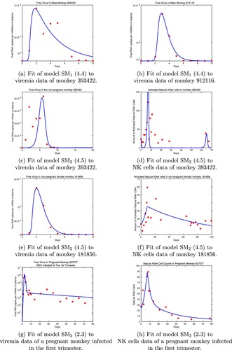
Figure 2. Fit of model (4(4) $\begin{array}{r}{\mathbf{W}\mathbf{i}\mathbf{t}\mathbf{h}\mathbf{i}\mathbf{n}\mathbf{-}\mathbf{v}\mathbf{e}\mathbf{c}\mathbf{t}\mathbf{o}\mathbf{r}\mathbf{m}\mathbf{o}\mathbf{d}\mathbf{e}\mathbf{l}\mathbf{(}\mathbf{M}}_4\mathbf{)}\mathbf{:}\left\{\begin{array}{ll}{P}_m^{\prime }& =r_m{P}_m(1-P_m/K_m)-m_t{P}_m,\\ P_s^{\prime }& =\frac{m_t{P}_m^2}{B+P_m^2}+r_s{P}_s(1-P_s/K_s),\end{array}\right.\end{array}$(4) ) to data in the midgut and salivary glands in the mosquito.

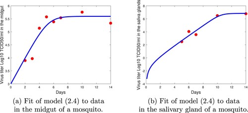
Table 3. Fitting results SM${}_1$, SM${}_2$, SM${}_3$, $M_4$.

Parameter	SM${}_1$ (393422)	SM${}_1$ (912116)	Unit
β	0.0008	0.000008	${\displaystyle \frac{ml}{\mathrm{v}\mathrm{R}\mathrm{N}\mathrm{A}\times \mathrm{d}\mathrm{a}\mathrm{y}}}$
δ	3.1675	1.5197	day${}^{-1}$
c	0.3192	1.5196	day${}^{-1}$
Parameter	SM${}_2$ (181856)	SM${}_2$ (393422)	Unit
β	0.0002	0.0006	${\displaystyle \frac{ml}{\mathrm{v}\mathrm{R}\mathrm{N}\mathrm{A}\times \mathrm{d}\mathrm{a}\mathrm{y}}}$
δ	0.0658	0.1483	${\displaystyle \frac{ml}{\mathrm{d}\mathrm{a}\mathrm{y}\times \mathrm{c}\mathrm{e}\mathrm{l}\mathrm{l}\mathrm{s}}}$
c	1.8875	0.2156	day${}^{-1}$
α	0.1320	0.2365	day${}^{-1}$
$\tilde{\gamma }$	48.9525	$1.7\times {10}^{-10}$	${\displaystyle \frac{{\mathrm{c}\mathrm{e}\mathrm{l}\mathrm{l}\mathrm{s}}^2}{{\mathrm{d}\mathrm{a}\mathrm{y}}^2}}$
d	0.0126	0.0277	day${}^{-1}$
Parameter	SM${}_3$(827577)	Unit
β	$5.05\times {10}^{-6}$	${\displaystyle \frac{ml}{\mathrm{v}\mathrm{R}\mathrm{N}\mathrm{A}\times \mathrm{d}\mathrm{a}\mathrm{y}}}$
δ	0.0426	${\displaystyle \frac{ml}{\mathrm{d}\mathrm{a}\mathrm{y}\times \mathrm{c}\mathrm{e}\mathrm{l}\mathrm{l}\mathrm{s}}}$
c	19.8990	day${}^{-1}$
α	0.4851	day${}^{-1}$
$\hat{\gamma }$	$1.4772\times {10}^5$	${\displaystyle \frac{{\mathrm{c}\mathrm{e}\mathrm{l}\mathrm{l}\mathrm{s}}^2}{{\mathrm{d}\mathrm{a}\mathrm{y}}^2}}$
d	0.2794	day${}^{-1}$
${\widehat{\text{β}}}_f$	$7.006\times {10}^{-6}$	day${}^{-1}$
$\hat{p}$	0.0563	day${}^{-1}$
$c_f$	0.0220	day${}^{-1}$

Table 4. Fitting Results $M_4$.

Parameter	$M_4$	Unit
$r_m$	1.26	day${}^{-1}$
$K_m$	$4.33\times {10}^5$	vRNA
$m_t$	0.11	day${}^{-1}$
B	$1.95\times {10}^4$	vRNA${}^2$
$r_s$	1.77	day${}^{-1}$
$K_s$	$6.84\times {10}^6$	vRNA

4. Structural identifiability analysis of within-host and within-vector models of Zika infection

Structural identifiability analysis examines whether the model parameters can be uniquely determined from the output function $g\left(\mathit{x}\right(t),\mathit{p})$, under ideal conditions such as noise-free data and error-free model. If the within-host model reveals all its parameters uniquely from the given output function, then the model (or its parameters) is said to be structurally (globally) identifiable. Structural identifiability analysis can be done without the actual experimental data, hence it is also called the prior identifiability analysis. When real data with noise is used to estimate the model parameters, a model which is structurally identifiable, might be unidentifiable in practice. It is crucial to check both structural and practical identifiability analysis of within-host and within-vector models before validating them with experimental data and using them for further insight. The definition of the structural identifiability is given as [27].

Definition 1

A parameter set $\mathit{p}$ is called structurally globally (or uniquely) identifiable if for every $\mathit{q}$ in the parameter space, the equation $g\left(\mathit{x}\right(t),\mathit{p})=g\left(\mathit{x}\right(t),\mathit{q})⟹\mathit{p}=\mathit{q}.$

That is any distinct parameter set yields different observations and hence the corresponding noise-free data are as well distinct.

Definition 2

Let $\mathcal{N}\left(\mathit{p}\right)$ denote the neighbourhood of the parameter $\mathit{p}$, then $\mathit{p}$ is called structurally locally identifiable if for every $\mathit{q}$ in the parameter space, the equation $g\left(\mathit{x}\right(t),\mathit{p})=g\left(\mathit{x}\right(t),\mathit{q})\mathrm{a}\mathrm{n}\mathrm{d}\mathit{q}\in \mathcal{N}\left(\mathit{p}\right)⟹\mathit{p}=\mathit{q}.$

There are many mathematical methods to study the structural identifiability of dynamic system ODE models. Some of these methods are differential algebra approach, Taylor series approach, generating series approach and a method based on the Implicit Function Theorem [5,13,25,27,37]. For details about these methods, we refer the reader to the good reviews written on the topic [11,27]. In this study, we use differential algebra approach to study the structural identifiability. We will briefly summarize the differential algebra approach here, but for more details reader is referred to [5,27]. The first step in differential algebra approach is to find the input–output equations of the system (5(5) $\begin{array}{r}\frac{d\mathit{x}}{dt}=f\left(\mathit{x}\right(t),\mathit{p})\mathit{x}\left(0\right)={\mathit{x}}_0\end{array}$(5) ), which is obtained by reducing the system to its characteristic set via Ritt's algorithm. The characteristic set of a dynamical system is not unique and it depends on the chosen ranking of the state variables. However, the coefficients of the input–output equation(s) can be fixed uniquely by normalizing the equation(s) to make them monic. The input–output equation(s) can also be obtained by eliminating the unobserved state variables. For instance, the observed state P of the model (1(1) $\begin{array}{r}{\mathbf{W}\mathbf{i}\mathbf{t}\mathbf{h}\mathbf{i}\mathbf{n}\mathbf{-}\mathbf{H}\mathbf{o}\mathbf{s}\mathbf{t}\mathbf{M}\mathbf{o}\mathbf{d}\mathbf{e}\mathbf{l}\mathbf{(}\mathbf{M}}_1\mathbf{)}\mathbf{:}\left\{\begin{array}{ll}{T}^{\prime }& =-\text{β}PT,\\ T_i^{\prime }& =\text{β}PT-\delta T_i,\\ P^{\prime }& =\pi T_i-cP.\end{array}\right.\end{array}$(1) ) satisfies the following differential algebraic equation, which we obtained by eliminating the unobservable state variables, T and $T_i$. (10) $\begin{array}{rl}& P^{‴}P-P^{″}{P}^{\prime }-\delta c{P}^{\prime }P-(\delta +c)(P^{\prime }{)}^2+\text{β}{P}^{″}{P}^2+\text{β}\delta c{P}^3\\ & +\text{β}(\delta +c)P^{\prime }{P}^2+\delta c{P}^{\prime }P+(\delta +c)P^{″}P=0\end{array}$(10) The input–output equation is a differential algebraic equation of the output, which in this case is the viremia level in plasma, $P\left(t\right)$ and its derivatives, with coefficients being the parameters of the model. The within-host model  (1(1) $\begin{array}{r}{\mathbf{W}\mathbf{i}\mathbf{t}\mathbf{h}\mathbf{i}\mathbf{n}\mathbf{-}\mathbf{H}\mathbf{o}\mathbf{s}\mathbf{t}\mathbf{M}\mathbf{o}\mathbf{d}\mathbf{e}\mathbf{l}\mathbf{(}\mathbf{M}}_1\mathbf{)}\mathbf{:}\left\{\begin{array}{ll}{T}^{\prime }& =-\text{β}PT,\\ T_i^{\prime }& =\text{β}PT-\delta T_i,\\ P^{\prime }& =\pi T_i-cP.\end{array}\right.\end{array}$(1) ) is said to be structurally identifiable if the map from the parameter space to the coefficients of the input–output equation is injective [13]. Thus the definition of the structural identifiability becomes

Definition 3

The dynamical model is structurally globally identifiable if and only if $c\left(\mathit{p}\right)=c\left(\mathit{q}\right)⟹\mathit{p}=\mathit{q}$ where $c\left(\mathit{p}\right)$ are the coefficients of the normalized input–output equation.

Suppose there exists a parameter set $\mathit{q}=[\widehat{\text{β}},\hat{\delta },\hat{\pi },\hat{c}]$ which produced the same observed state P. Then, equalling the coefficients of the differential algebraic equation (10(10) $\begin{array}{rl}& P^{‴}P-P^{″}{P}^{\prime }-\delta c{P}^{\prime }P-(\delta +c)(P^{\prime }{)}^2+\text{β}{P}^{″}{P}^2+\text{β}\delta c{P}^3\\ & +\text{β}(\delta +c)P^{\prime }{P}^2+\delta c{P}^{\prime }P+(\delta +c)P^{″}P=0\end{array}$(10) ), we obtain (11) $\begin{array}{r}\text{β}=\widehat{\text{β}},\delta c=\hat{\delta }\hat{c},\delta +c=\hat{\delta }+\hat{c}\end{array}$(11) Solving the nonlinear equation system (11(11) $\begin{array}{r}\text{β}=\widehat{\text{β}},\delta c=\hat{\delta }\hat{c},\delta +c=\hat{\delta }+\hat{c}\end{array}$(11) ), results in two sets of solutions, $\text{β}=\widehat{\text{β}},\delta =\hat{\delta },c=\hat{c}\mathrm{o}\mathrm{r}\text{β}=\widehat{\text{β}},\delta =\hat{c},c=\hat{\delta }.$ Hence, the model parameters δ and c are only locally identifiable from viral load observations. On the other hand, the parameter π does not appear in the input-output equation (10(10) $\begin{array}{rl}& P^{‴}P-P^{″}{P}^{\prime }-\delta c{P}^{\prime }P-(\delta +c)(P^{\prime }{)}^2+\text{β}{P}^{″}{P}^2+\text{β}\delta c{P}^3\\ & +\text{β}(\delta +c)P^{\prime }{P}^2+\delta c{P}^{\prime }P+(\delta +c)P^{″}P=0\end{array}$(10) ). Hence it is not identifiable. This could also be seen by scaling the unobserved state variables by σ: $x=\sigma T,y=\sigma T_i,z=V$. We obtain (12) $\begin{array}{r}\mathbf{W}\mathbf{i}\mathbf{t}\mathbf{h}\mathbf{i}\mathbf{n}\mathbf{i}\mathbf{n}\mathbf{f}\mathbf{e}\mathbf{c}\mathbf{t}\mathbf{e}\mathbf{d}\mathbf{h}\mathbf{o}\mathbf{s}\mathbf{t}\mathbf{m}\mathbf{o}\mathbf{d}\mathbf{e}\mathbf{l}\mathbf{:}\left\{\begin{array}{ll}{x}^{\prime }& =-\text{β}zx,\\ y^{\prime }& =\text{β}zx-\delta y,\\ z^{\prime }& =\hat{\pi }y-cz,\end{array}\right.\end{array}$(12) Thus $(T,T_i,P)$ solves the system (1(1) $\begin{array}{r}{\mathbf{W}\mathbf{i}\mathbf{t}\mathbf{h}\mathbf{i}\mathbf{n}\mathbf{-}\mathbf{H}\mathbf{o}\mathbf{s}\mathbf{t}\mathbf{M}\mathbf{o}\mathbf{d}\mathbf{e}\mathbf{l}\mathbf{(}\mathbf{M}}_1\mathbf{)}\mathbf{:}\left\{\begin{array}{ll}{T}^{\prime }& =-\text{β}PT,\\ T_i^{\prime }& =\text{β}PT-\delta T_i,\\ P^{\prime }& =\pi T_i-cP.\end{array}\right.\end{array}$(1) ) and $(\sigma T,\sigma T_i,P)$ solves the system (12(12) $\begin{array}{r}\mathbf{W}\mathbf{i}\mathbf{t}\mathbf{h}\mathbf{i}\mathbf{n}\mathbf{i}\mathbf{n}\mathbf{f}\mathbf{e}\mathbf{c}\mathbf{t}\mathbf{e}\mathbf{d}\mathbf{h}\mathbf{o}\mathbf{s}\mathbf{t}\mathbf{m}\mathbf{o}\mathbf{d}\mathbf{e}\mathbf{l}\mathbf{:}\left\{\begin{array}{ll}{x}^{\prime }& =-\text{β}zx,\\ y^{\prime }& =\text{β}zx-\delta y,\\ z^{\prime }& =\hat{\pi }y-cz,\end{array}\right.\end{array}$(12) ) where $\hat{\pi }={\displaystyle \frac{\pi }{\sigma }}$. Hence, π is not identifiable from the viral load observations. Thus we have proven the following proposition:

Proposition 1

The within-host model (1(1) $\begin{array}{r}{\mathbf{W}\mathbf{i}\mathbf{t}\mathbf{h}\mathbf{i}\mathbf{n}\mathbf{-}\mathbf{H}\mathbf{o}\mathbf{s}\mathbf{t}\mathbf{M}\mathbf{o}\mathbf{d}\mathbf{e}\mathbf{l}\mathbf{(}\mathbf{M}}_1\mathbf{)}\mathbf{:}\left\{\begin{array}{ll}{T}^{\prime }& =-\text{β}PT,\\ T_i^{\prime }& =\text{β}PT-\delta T_i,\\ P^{\prime }& =\pi T_i-cP.\end{array}\right.\end{array}$(1) ) is not structurally identifiable from the viremia observations. Only the parameter β is structurally identifiable, parameters δ and c are only locally structurally identifiable and the parameter π is not identifiable from the viremia observations.

Both the structural and practical identifiability of the target cell-limited model (1(1) $\begin{array}{r}{\mathbf{W}\mathbf{i}\mathbf{t}\mathbf{h}\mathbf{i}\mathbf{n}\mathbf{-}\mathbf{H}\mathbf{o}\mathbf{s}\mathbf{t}\mathbf{M}\mathbf{o}\mathbf{d}\mathbf{e}\mathbf{l}\mathbf{(}\mathbf{M}}_1\mathbf{)}\mathbf{:}\left\{\begin{array}{ll}{T}^{\prime }& =-\text{β}PT,\\ T_i^{\prime }& =\text{β}PT-\delta T_i,\\ P^{\prime }& =\pi T_i-cP.\end{array}\right.\end{array}$(1) ) have been studied extensively [28,40]. In summary, the model parameters δ and c are only locally identifiable from viral load observations, while the parameter π is not identifiable. Since, (1(1) $\begin{array}{r}{\mathbf{W}\mathbf{i}\mathbf{t}\mathbf{h}\mathbf{i}\mathbf{n}\mathbf{-}\mathbf{H}\mathbf{o}\mathbf{s}\mathbf{t}\mathbf{M}\mathbf{o}\mathbf{d}\mathbf{e}\mathbf{l}\mathbf{(}\mathbf{M}}_1\mathbf{)}\mathbf{:}\left\{\begin{array}{ll}{T}^{\prime }& =-\text{β}PT,\\ T_i^{\prime }& =\text{β}PT-\delta T_i,\\ P^{\prime }& =\pi T_i-cP.\end{array}\right.\end{array}$(1) ) is not structurally identifiable, we scale the unobserved state variables, target cells and infected target cell with the unidentifiable parameter, π to obtain a structurally identifiable model, (13) $\begin{array}{r}{\mathbf{S}\mathbf{c}\mathbf{a}\mathbf{l}\mathbf{e}\mathbf{d}\mathbf{w}\mathbf{i}\mathbf{t}\mathbf{h}\mathbf{i}\mathbf{n}\mathbf{-}\mathbf{h}\mathbf{o}\mathbf{s}\mathbf{t}\mathbf{M}\mathbf{o}\mathbf{d}\mathbf{e}\mathbf{l}\mathbf{(}\mathbf{S}\mathbf{M}}_1\mathbf{)}\mathbf{:}\left\{\begin{array}{ll}{\hat{T}}^{\prime }& =-\text{β}P\hat{T},\\ {\hat{T}}_i^{\prime }& =\text{β}P\hat{T}-\delta {\hat{T}}_i,\\ P^{\prime }& ={\hat{T}}_i-cP,\end{array}\right.\end{array}$(13) where $\hat{T}=\pi T$ and ${\hat{T}}_i=\pi T_i$. The scaled within-host model (13(13) $\begin{array}{r}{\mathbf{S}\mathbf{c}\mathbf{a}\mathbf{l}\mathbf{e}\mathbf{d}\mathbf{w}\mathbf{i}\mathbf{t}\mathbf{h}\mathbf{i}\mathbf{n}\mathbf{-}\mathbf{h}\mathbf{o}\mathbf{s}\mathbf{t}\mathbf{M}\mathbf{o}\mathbf{d}\mathbf{e}\mathbf{l}\mathbf{(}\mathbf{S}\mathbf{M}}_1\mathbf{)}\mathbf{:}\left\{\begin{array}{ll}{\hat{T}}^{\prime }& =-\text{β}P\hat{T},\\ {\hat{T}}_i^{\prime }& =\text{β}P\hat{T}-\delta {\hat{T}}_i,\\ P^{\prime }& ={\hat{T}}_i-cP,\end{array}\right.\end{array}$(13) ) is locally identifiable. In this model, π essentially has value 1 and similar investigations as before show that δ and c are locally identifiable.

Next, we study the structural identifiability of the within-host model (2(2) $\begin{array}{r}{\mathbf{W}\mathbf{i}\mathbf{t}\mathbf{h}\mathbf{i}\mathbf{n}\mathbf{-}\mathbf{H}\mathbf{o}\mathbf{s}\mathbf{t}\mathbf{M}\mathbf{o}\mathbf{d}\mathbf{e}\mathbf{l}\mathbf{w}\mathbf{i}\mathbf{t}\mathbf{h}\mathbf{I}\mathbf{m}\mathbf{m}\mathbf{u}\mathbf{n}\mathbf{e}\mathbf{R}\mathbf{e}\mathbf{s}\mathbf{p}\mathbf{o}\mathbf{n}\mathbf{s}\mathbf{e}\mathbf{(}\mathbf{M}}_2\mathbf{)}\mathbf{:}\left\{\begin{array}{ll}{T}^{\prime }& =-\text{β}PT,\\ T_i^{\prime }& =\text{β}PT-\delta T_{i}N,\\ P^{\prime }& =\pi T_i-cP,\\ N^{\prime }& =\frac{\alpha T_i^{2}N}{T_i^2+\gamma }-dN.\end{array}\right.\end{array}$(2) ). Even though data for two state variables are available, model (2(2) $\begin{array}{r}{\mathbf{W}\mathbf{i}\mathbf{t}\mathbf{h}\mathbf{i}\mathbf{n}\mathbf{-}\mathbf{H}\mathbf{o}\mathbf{s}\mathbf{t}\mathbf{M}\mathbf{o}\mathbf{d}\mathbf{e}\mathbf{l}\mathbf{w}\mathbf{i}\mathbf{t}\mathbf{h}\mathbf{I}\mathbf{m}\mathbf{m}\mathbf{u}\mathbf{n}\mathbf{e}\mathbf{R}\mathbf{e}\mathbf{s}\mathbf{p}\mathbf{o}\mathbf{n}\mathbf{s}\mathbf{e}\mathbf{(}\mathbf{M}}_2\mathbf{)}\mathbf{:}\left\{\begin{array}{ll}{T}^{\prime }& =-\text{β}PT,\\ T_i^{\prime }& =\text{β}PT-\delta T_{i}N,\\ P^{\prime }& =\pi T_i-cP,\\ N^{\prime }& =\frac{\alpha T_i^{2}N}{T_i^2+\gamma }-dN.\end{array}\right.\end{array}$(2) ) is not identifiable.

Proposition 2

The within-host model (2(2) $\begin{array}{r}{\mathbf{W}\mathbf{i}\mathbf{t}\mathbf{h}\mathbf{i}\mathbf{n}\mathbf{-}\mathbf{H}\mathbf{o}\mathbf{s}\mathbf{t}\mathbf{M}\mathbf{o}\mathbf{d}\mathbf{e}\mathbf{l}\mathbf{w}\mathbf{i}\mathbf{t}\mathbf{h}\mathbf{I}\mathbf{m}\mathbf{m}\mathbf{u}\mathbf{n}\mathbf{e}\mathbf{R}\mathbf{e}\mathbf{s}\mathbf{p}\mathbf{o}\mathbf{n}\mathbf{s}\mathbf{e}\mathbf{(}\mathbf{M}}_2\mathbf{)}\mathbf{:}\left\{\begin{array}{ll}{T}^{\prime }& =-\text{β}PT,\\ T_i^{\prime }& =\text{β}PT-\delta T_{i}N,\\ P^{\prime }& =\pi T_i-cP,\\ N^{\prime }& =\frac{\alpha T_i^{2}N}{T_i^2+\gamma }-dN.\end{array}\right.\end{array}$(2) ) is not structurally identifiable from the viremia observations and activated NK cell counts. Only the parameters $\text{β},\delta ,c,\alpha$ and d are identifiable. The parameters π and γ are not identifiable, but the parameter combination ${\pi }^2\gamma$ is identifiable from the observations of viremia load and activated NK cell counts.

Proof.

We obtain the input–output equations using the software package Differential Algebra for Identifiability of Systems (DAISY) [5]. DAISY gives the differential algebraic equations for the observed state variables P and N which are presented in Appendix. Solving $c\left(\mathit{p}\right)=c\left(\mathit{q}\right)$ where $\mathit{p}=[\text{β},\delta ,\pi ,c,\alpha ,\gamma ,d]$ and $\mathit{q}=[\widehat{\text{β}},\hat{\delta },\hat{\pi },\hat{c},\hat{\alpha },\hat{\gamma },\hat{d}]$ we obtain, $\text{β}=\widehat{\text{β}},\delta =\hat{\delta },{\pi }^2\gamma ={\hat{\pi }}^2\hat{\gamma },c=\hat{c},\alpha =\hat{\alpha },d=\hat{d}$

We scale the unobserved state variables, target cells and infected target cells with the unidentifiable parameter, π by $\hat{T}=\pi T$ and ${\hat{T}}_i=\pi T_i$ and obtain the following scaled model of (2(2) $\begin{array}{r}{\mathbf{W}\mathbf{i}\mathbf{t}\mathbf{h}\mathbf{i}\mathbf{n}\mathbf{-}\mathbf{H}\mathbf{o}\mathbf{s}\mathbf{t}\mathbf{M}\mathbf{o}\mathbf{d}\mathbf{e}\mathbf{l}\mathbf{w}\mathbf{i}\mathbf{t}\mathbf{h}\mathbf{I}\mathbf{m}\mathbf{m}\mathbf{u}\mathbf{n}\mathbf{e}\mathbf{R}\mathbf{e}\mathbf{s}\mathbf{p}\mathbf{o}\mathbf{n}\mathbf{s}\mathbf{e}\mathbf{(}\mathbf{M}}_2\mathbf{)}\mathbf{:}\left\{\begin{array}{ll}{T}^{\prime }& =-\text{β}PT,\\ T_i^{\prime }& =\text{β}PT-\delta T_{i}N,\\ P^{\prime }& =\pi T_i-cP,\\ N^{\prime }& =\frac{\alpha T_i^{2}N}{T_i^2+\gamma }-dN.\end{array}\right.\end{array}$(2) ) (14) $\begin{array}{r}{\mathbf{S}\mathbf{c}\mathbf{a}\mathbf{l}\mathbf{e}\mathbf{d}\mathbf{w}\mathbf{i}\mathbf{t}\mathbf{h}\mathbf{i}\mathbf{n}\mathbf{-}\mathbf{h}\mathbf{o}\mathbf{s}\mathbf{t}\mathbf{M}\mathbf{o}\mathbf{d}\mathbf{e}\mathbf{l}\mathbf{2}\mathbf{(}\mathbf{S}\mathbf{M}}_2\mathbf{)}\mathbf{:}\left\{\begin{array}{ll}{\hat{T}}^{\prime }& =-\text{β}P\hat{T},\\ {\hat{T}}_i^{\prime }& =\text{β}P\hat{T}-\delta {\hat{T}}_{i}N,\\ P^{\prime }& ={\hat{T}}_i-cP,\\ N^{\prime }& =\frac{\alpha {\hat{T}}_i^{2}N}{{\hat{T}}_i^2+\tilde{\gamma }}-dN,\end{array}\right.\end{array}$(14) where $\tilde{\gamma }={\pi }^2\gamma$. The scaled within-host model (14(14) $\begin{array}{r}{\mathbf{S}\mathbf{c}\mathbf{a}\mathbf{l}\mathbf{e}\mathbf{d}\mathbf{w}\mathbf{i}\mathbf{t}\mathbf{h}\mathbf{i}\mathbf{n}\mathbf{-}\mathbf{h}\mathbf{o}\mathbf{s}\mathbf{t}\mathbf{M}\mathbf{o}\mathbf{d}\mathbf{e}\mathbf{l}\mathbf{2}\mathbf{(}\mathbf{S}\mathbf{M}}_2\mathbf{)}\mathbf{:}\left\{\begin{array}{ll}{\hat{T}}^{\prime }& =-\text{β}P\hat{T},\\ {\hat{T}}_i^{\prime }& =\text{β}P\hat{T}-\delta {\hat{T}}_{i}N,\\ P^{\prime }& ={\hat{T}}_i-cP,\\ N^{\prime }& =\frac{\alpha {\hat{T}}_i^{2}N}{{\hat{T}}_i^2+\tilde{\gamma }}-dN,\end{array}\right.\end{array}$(14) ) is structurally identifiable because the parameter $\tilde{\gamma }$ is identifiable and the remaining parameters are identifiable.

Next, we study the structural identifiability of within pregnant host model, $M_3$. However, obtaining an input–output equation for the observed state variable P and N for model $M_3$ using DAISY was computationally expensive. Therefore, we use the Identifiability Analysis package in MATHEMATICA to test for the local identifiability of the within pregnant host model $M_3$. For detailed information on Identifiability Analysis package in MATHEMATICA, we refer to [20]. The Identifiability Analysis package gives that the parameters ${\text{β}}_f,\delta ,\gamma ,\pi ,p_f,{\pi }_f,p$ of the within pregnant host model $M_3$ cannot be identified from the viremia observations and activated NK cell counts. To obtain a model whose parameters are identifiable, we scale the unobserved state variables as $\hat{T}=\pi T$, ${\hat{T}}_i=\pi T_i$,$\hat{H}={\pi }_{f}H$, ${\hat{H}}_i={\pi }_f{H}_i$ and ${\hat{P}}_f=p_f{P}_f$ and get (15) $\begin{array}{r}{\mathbf{S}\mathbf{c}\mathbf{a}\mathbf{l}\mathbf{e}\mathbf{d}\mathbf{W}\mathbf{i}\mathbf{t}\mathbf{h}\mathbf{i}\mathbf{n}\mathbf{P}\mathbf{r}\mathbf{e}\mathbf{g}\mathbf{n}\mathbf{a}\mathbf{n}\mathbf{t}\mathbf{H}\mathbf{o}\mathbf{s}\mathbf{t}\mathbf{M}\mathbf{o}\mathbf{d}\mathbf{e}\mathbf{l}\mathbf{(}\mathbf{S}\mathbf{M}}_3\mathbf{)}\mathbf{:}\left\{\begin{array}{ll}{\hat{T}}^{\prime }& =-\text{β}P\hat{T},\\ {\hat{T}}_i^{\prime }& =\text{β}P\hat{T}-\delta {\hat{T}}_{i}N,\\ P^{\prime }& ={\hat{T}}_i+{\hat{P}}_f-cP,\\ N^{\prime }& =\frac{\alpha {\hat{T}}_i^{2}N}{{\hat{T}}_i^2+\hat{\gamma }}-dN,\\ {\hat{H}}^{\prime }& =-{\widehat{\text{β}}}_f{\hat{P}}_f\hat{H},\\ {\hat{H}}_i^{\prime }& ={\widehat{\text{β}}}_f{\hat{P}}_f\hat{H}-{\delta }_f{\hat{H}}_i,\\ {\hat{P}}_f^{\prime }& =\hat{p}P+{\hat{H}}_i-c_f{\hat{P}}_f,\end{array}\right.\end{array}$(15) where $\hat{\gamma }={\pi }^2\gamma ,\hat{p}=p{p}_f,{\widehat{\text{β}}}_f={\displaystyle \frac{{\text{β}}_f}{p_f}}$. The Identifiability Analysis package gives that the scaled model SM${}_3$ is locally identifiable.

Finally, we test the identifiability of the within-vector model. When composing the model, we were very careful with the number of classes and we included only as many classes as data sets. We expect that would improve the structural identifiability of the model. Indeed the next proposition states that the within-vector model is structurally identifiable.

Proposition 3

The within-vector model (4(4) $\begin{array}{r}{\mathbf{W}\mathbf{i}\mathbf{t}\mathbf{h}\mathbf{i}\mathbf{n}\mathbf{-}\mathbf{v}\mathbf{e}\mathbf{c}\mathbf{t}\mathbf{o}\mathbf{r}\mathbf{m}\mathbf{o}\mathbf{d}\mathbf{e}\mathbf{l}\mathbf{(}\mathbf{M}}_4\mathbf{)}\mathbf{:}\left\{\begin{array}{ll}{P}_m^{\prime }& =r_m{P}_m(1-P_m/K_m)-m_t{P}_m,\\ P_s^{\prime }& =\frac{m_t{P}_m^2}{B+P_m^2}+r_s{P}_s(1-P_s/K_s),\end{array}\right.\end{array}$(4) ) is structurally identifiable from the viremia observations in the midgut and salivary glands.

Proof: The following differential algebraic equations for the observed state variables $P_m$ and $P_s$ can be easily obtained from  (4(4) $\begin{array}{r}{\mathbf{W}\mathbf{i}\mathbf{t}\mathbf{h}\mathbf{i}\mathbf{n}\mathbf{-}\mathbf{v}\mathbf{e}\mathbf{c}\mathbf{t}\mathbf{o}\mathbf{r}\mathbf{m}\mathbf{o}\mathbf{d}\mathbf{e}\mathbf{l}\mathbf{(}\mathbf{M}}_4\mathbf{)}\mathbf{:}\left\{\begin{array}{ll}{P}_m^{\prime }& =r_m{P}_m(1-P_m/K_m)-m_t{P}_m,\\ P_s^{\prime }& =\frac{m_t{P}_m^2}{B+P_m^2}+r_s{P}_s(1-P_s/K_s),\end{array}\right.\end{array}$(4) ), (16) $\begin{array}{r}{P}_m^{\prime }+P_m^2\frac{r_m}{K_m}+P_m(m_t-r_m)=0\end{array}$(16) and (17) $\begin{array}{r}{P}_s^{\prime }{P}_m^2+B{P}_s^{\prime }+\frac{r_s}{K_s}{P}_s^2-r_s{P}_m^2{P}_s-m_t{P}_m^2+\frac{B{r}_s}{K_s}{P}_s^2-B{r}_s{P}_s=0\end{array}$(17) Solving $c\left(\mathit{p}\right)=c\left(\mathit{q}\right)$ where $\mathit{p}=[r_m,K_m,m_t,B,r_s,K_s]$ and $\mathit{q}=[{\hat{r}}_m,{\hat{K}}_m,{\hat{m}}_t,\hat{B},{\hat{r}}_s,{\hat{K}}_s]$ we obtain the following solution, $r_m={\hat{r}}_m,K_m={\hat{K}}_m,m_t={\hat{m}}_t,B=\hat{B},r_s={\hat{r}}_s,K_s={\hat{K}}_s$

5. Practical identifiability analysis of within-host and within-vector models of Zika infection

We first perform global sensitivity analysis by using Latin hypercube sampling (LHS) method to determine the key factors that affect the peak Zika viral load [26]. Banarjee et al. determined the range of biological parameters of within-host mathematical models of WNV which describe viral replication, spread and host immune response in wild-type and immunocompromised mice [1]. The viral production rate, π, of flavivirus is low, ranges between [0.3,120] [1], compared to HIV, which is estimated as $3.26\times {10}^4$ [19]. To perform the global sensitivity analysis, the parameters of the model (2(2) $\begin{array}{r}{\mathbf{W}\mathbf{i}\mathbf{t}\mathbf{h}\mathbf{i}\mathbf{n}\mathbf{-}\mathbf{H}\mathbf{o}\mathbf{s}\mathbf{t}\mathbf{M}\mathbf{o}\mathbf{d}\mathbf{e}\mathbf{l}\mathbf{w}\mathbf{i}\mathbf{t}\mathbf{h}\mathbf{I}\mathbf{m}\mathbf{m}\mathbf{u}\mathbf{n}\mathbf{e}\mathbf{R}\mathbf{e}\mathbf{s}\mathbf{p}\mathbf{o}\mathbf{n}\mathbf{s}\mathbf{e}\mathbf{(}\mathbf{M}}_2\mathbf{)}\mathbf{:}\left\{\begin{array}{ll}{T}^{\prime }& =-\text{β}PT,\\ T_i^{\prime }& =\text{β}PT-\delta T_{i}N,\\ P^{\prime }& =\pi T_i-cP,\\ N^{\prime }& =\frac{\alpha T_i^{2}N}{T_i^2+\gamma }-dN.\end{array}\right.\end{array}$(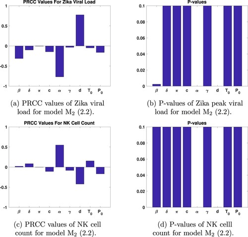2) ) are sampled randomly using uniform distribution whose range is given in [1]. The sample size is set to 1000. Partial rank correlation coefficients (PRCC) [26] and their p-values are given in Figure 3. PRCC results show that Zika viral load and NK cell count are most sensitive to d, clearance rate of the NK cells and α – immune response activation rate. As seen from Figure 3, the infectious rate of susceptible target cells also has significant impact on the output (p-value $<0.05$). On the other hand, peak viral load is not very sensitive to initial viral load or initial number of target cell. Insensitivity of the viremia level of the infected host to the initial viral load has also been established previously [1,40]. Sensitivity analysis of model (2(2) $\begin{array}{r}{\mathbf{W}\mathbf{i}\mathbf{t}\mathbf{h}\mathbf{i}\mathbf{n}\mathbf{-}\mathbf{H}\mathbf{o}\mathbf{s}\mathbf{t}\mathbf{M}\mathbf{o}\mathbf{d}\mathbf{e}\mathbf{l}\mathbf{w}\mathbf{i}\mathbf{t}\mathbf{h}\mathbf{I}\mathbf{m}\mathbf{m}\mathbf{u}\mathbf{n}\mathbf{e}\mathbf{R}\mathbf{e}\mathbf{s}\mathbf{p}\mathbf{o}\mathbf{n}\mathbf{s}\mathbf{e}\mathbf{(}\mathbf{M}}_2\mathbf{)}\mathbf{:}\left\{\begin{array}{ll}{T}^{\prime }& =-\text{β}PT,\\ T_i^{\prime }& =\text{β}PT-\delta T_{i}N,\\ P^{\prime }& =\pi T_i-cP,\\ N^{\prime }& =\frac{\alpha T_i^{2}N}{T_i^2+\gamma }-dN.\end{array}\right.\end{array}$(2) ) based on LHS shows that only the parameters α and d have PRCC values greater than 0.5 or less than $-0.5$ for both viral load and NK cell counts (see Figure 3 (a) and (c)). On the other hand, Zika viral load and NK cell counts are not sensitive to γ, π, $P_0$ or $T_0$.

Figure 3. PRCC and P-values of model (2(2) $\begin{array}{r}{\mathbf{W}\mathbf{i}\mathbf{t}\mathbf{h}\mathbf{i}\mathbf{n}\mathbf{-}\mathbf{H}\mathbf{o}\mathbf{s}\mathbf{t}\mathbf{M}\mathbf{o}\mathbf{d}\mathbf{e}\mathbf{l}\mathbf{w}\mathbf{i}\mathbf{t}\mathbf{h}\mathbf{I}\mathbf{m}\mathbf{m}\mathbf{u}\mathbf{n}\mathbf{e}\mathbf{R}\mathbf{e}\mathbf{s}\mathbf{p}\mathbf{o}\mathbf{n}\mathbf{s}\mathbf{e}\mathbf{(}\mathbf{M}}_2\mathbf{)}\mathbf{:}\left\{\begin{array}{ll}{T}^{\prime }& =-\text{β}PT,\\ T_i^{\prime }& =\text{β}PT-\delta T_{i}N,\\ P^{\prime }& =\pi T_i-cP,\\ N^{\prime }& =\frac{\alpha T_i^{2}N}{T_i^2+\gamma }-dN.\end{array}\right.\end{array}$(2) ) parameters.

To further analyse the identifiability of the models, we perform Monte Carlo simulations which have been widely used for practical identifiability of ODE models [27,43]. We generate 1000 synthetic data sets using the true parameter set $\hat{\mathit{p}}$ and adding noise at increasing levels. The true parameter set $\hat{\mathit{p}}$ for each model is obtained through the fitting to the data [48] and is as given in Table 3 and Table 4. We outline the Monte Carlo simulations in the following steps.

1. Solve the within-host and within-vector models, SM${}_1$, SM${}_2$, SM${}_3$, and M${}_4$ numerically with the true parameters $\hat{\mathit{p}}$ and obtain the output vector $\mathit{g}\left(\mathit{x}\right(t),\hat{\mathit{p}})$ at the discrete data time points $\{t_i{\}}_{i=1}^n.$

2. Generate M = 1000 data sets from the statistical model (6(6) $\begin{array}{r}{y}_i=g\left(\mathit{x}\right(t_i),\hat{\mathit{p}})+E_i\end{array}$(6) ) with a given measurement error. Data sets are drawn from a normal distribution whose mean is the output vector obtained in step ( 1) and standard deviation is the ${\sigma }_0\mathrm{\%}$ of the mean. That is, we set $\xi =1$ in the error structure given in (6(6) $\begin{array}{r}{y}_i=g\left(\mathit{x}\right(t_i),\hat{\mathit{p}})+E_i\end{array}$(6) ) $y_i=g\left(\mathit{x}\right(t_i),\hat{\mathit{p}})+g\left(\mathit{x}\right(t_i),\hat{\mathit{p}}){ϵ}_{i}i=1,2,\dots ,n.$ Hence, the random variables $y_i$ have mean $\mathbb{E}\left(y_i\right)=g\left(\mathit{x}\right(t_i),\hat{\mathit{p}})$ and variances $Var\left(y_i\right)=g\left(\mathit{x}\right(t_i),\hat{\mathit{p}}{)}^2{\sigma }_0^2$.

3. Fit the model ${\mathit{x}}^{\prime }=f(\mathit{x},t,\mathit{p}),\mathit{x}\left(0\right)={\mathit{x}}_0$ to each of the M simulated data sets to estimate the parameter set ${\mathit{p}}_j$ for $j=1,2,\dots ,M$. That is ${\mathit{p}}_j=\underset{\mathit{p}}{min}\sum _{i=1}^n{\left(y_i-g\left(\mathit{x}\right(t_i),\mathit{p})\right)}^2,j=1,2,\dots ,M.$

4. Calculate the average relative estimation error for each parameter in the set $\mathit{p}$ by [27] $ARE\left(p^{\left(k\right)}\right)=100\mathrm{\%}\frac{1}{M}\sum _{j=1}^M\frac{|{\hat{p}}^{\left(k\right)}-p_j^{\left(k\right)}|}{{\hat{p}}^{\left(k\right)}}$ where $p^{\left(k\right)}$ is the $k^{th}$ parameter in the set $\mathit{p}$, ${\hat{p}}^{\left(k\right)}$ is the $k^{th}$ parameter in the true parameter set $\hat{\mathit{p}}$, and $p_j^{\left(k\right)}$ is the $k^{th}$ parameter in the set ${\mathit{p}}_j$.

5. Repeat steps 1 through 5 with increasing level of noise, that is take ${\sigma }_0=0,1,5,10,$ $20,30\mathrm{\%}.$

We perform Monte Carlo simulations by generating 1000 random data sets for each measurement error level, and fitting each data set to the within-host or within-vector model. We then compute the average relative estimation errors (ARE) for each parameter in the model. AREs give us insight about how much the estimated parameters are sensitive to the noise in the data. When ${\sigma }_0=0$, that is when there is no noise in the data, the AREs of the estimated parameters of a structurally (globally) identifiable model should be 0 or very close to 0. As the noise level in the data increases, the AREs of the model parameters increase as well. If a parameter is not practically identifiable, then the AREs of that parameter will be significantly high even for a reasonable level of measurement error. Some of the parameters will be very sensitive to the noise in the data, and increasing the measurement errors will result in significantly higher AREs. In this case, we claim that the parameter is practically unidentifiable. If the AREs of the parameter are lower than the measurement error ${\sigma }_0$ or higher at least a couple of times, then we say that the parameter is practically identifiable.

Monte Carlo simulations that compute AREs give a local identifiability result. Looking at Table 5 and AREs of scaled model SM${}_1$, we see that the AREs of the estimated parameters of SM${}_1$ from the monkey 393422 are smaller than the measurement error ${\sigma }_0$. That is we conclude that parameters of SM${}_1$ are practically identifiable. As for the second data set (monkey 912116), we see that not all the AREs are less than the measurement error ${\sigma }_0$ (see AREs of parameters δ and c). But AREs are controlled and we still conclude that the scaled target limited cell model is practically identifiable. Next, consider the practical identifiability of scaled within-host model (14(14) $\begin{array}{r}{\mathbf{S}\mathbf{c}\mathbf{a}\mathbf{l}\mathbf{e}\mathbf{d}\mathbf{w}\mathbf{i}\mathbf{t}\mathbf{h}\mathbf{i}\mathbf{n}\mathbf{-}\mathbf{h}\mathbf{o}\mathbf{s}\mathbf{t}\mathbf{M}\mathbf{o}\mathbf{d}\mathbf{e}\mathbf{l}\mathbf{2}\mathbf{(}\mathbf{S}\mathbf{M}}_2\mathbf{)}\mathbf{:}\left\{\begin{array}{ll}{\hat{T}}^{\prime }& =-\text{β}P\hat{T},\\ {\hat{T}}_i^{\prime }& =\text{β}P\hat{T}-\delta {\hat{T}}_{i}N,\\ P^{\prime }& ={\hat{T}}_i-cP,\\ N^{\prime }& =\frac{\alpha {\hat{T}}_i^{2}N}{{\hat{T}}_i^2+\tilde{\gamma }}-dN,\end{array}\right.\end{array}$(14) ). Looking at Table 6 and Table 7 we see that with the exception of $\tilde{\gamma }$ all other parameters have AREs smaller than the measurement error ${\sigma }_0$, or AREs are slightly higher but we can still conclude that the parameters $\text{β},\delta ,c,\alpha$ and d are practically identifiable. However, the AREs of $\tilde{\gamma }$ are so high that we conclude that $\tilde{\gamma }$ is not practically identifiable. Actually, this phenomenon is observed quite often: when we ‘fold in’ a structurally unidentifiable parameter into a structurally identifiable parameter, then this structurally identifiable parameter that embeds an unidentifiable parameter fails to be practically identifiable, as is the case with $\tilde{\gamma }$. Finally from the within-host models, we performed the Monte Carlo simulations for the scaled model (15(15) $\begin{array}{r}{\mathbf{S}\mathbf{c}\mathbf{a}\mathbf{l}\mathbf{e}\mathbf{d}\mathbf{W}\mathbf{i}\mathbf{t}\mathbf{h}\mathbf{i}\mathbf{n}\mathbf{P}\mathbf{r}\mathbf{e}\mathbf{g}\mathbf{n}\mathbf{a}\mathbf{n}\mathbf{t}\mathbf{H}\mathbf{o}\mathbf{s}\mathbf{t}\mathbf{M}\mathbf{o}\mathbf{d}\mathbf{e}\mathbf{l}\mathbf{(}\mathbf{S}\mathbf{M}}_3\mathbf{)}\mathbf{:}\left\{\begin{array}{ll}{\hat{T}}^{\prime }& =-\text{β}P\hat{T},\\ {\hat{T}}_i^{\prime }& =\text{β}P\hat{T}-\delta {\hat{T}}_{i}N,\\ P^{\prime }& ={\hat{T}}_i+{\hat{P}}_f-cP,\\ N^{\prime }& =\frac{\alpha {\hat{T}}_i^{2}N}{{\hat{T}}_i^2+\hat{\gamma }}-dN,\\ {\hat{H}}^{\prime }& =-{\widehat{\text{β}}}_f{\hat{P}}_f\hat{H},\\ {\hat{H}}_i^{\prime }& ={\widehat{\text{β}}}_f{\hat{P}}_f\hat{H}-{\delta }_f{\hat{H}}_i,\\ {\hat{P}}_f^{\prime }& =\hat{p}P+{\hat{H}}_i-c_f{\hat{P}}_f,\end{array}\right.\end{array}$(15) ). Even though the scaled model (15(15) $\begin{array}{r}{\mathbf{S}\mathbf{c}\mathbf{a}\mathbf{l}\mathbf{e}\mathbf{d}\mathbf{W}\mathbf{i}\mathbf{t}\mathbf{h}\mathbf{i}\mathbf{n}\mathbf{P}\mathbf{r}\mathbf{e}\mathbf{g}\mathbf{n}\mathbf{a}\mathbf{n}\mathbf{t}\mathbf{H}\mathbf{o}\mathbf{s}\mathbf{t}\mathbf{M}\mathbf{o}\mathbf{d}\mathbf{e}\mathbf{l}\mathbf{(}\mathbf{S}\mathbf{M}}_3\mathbf{)}\mathbf{:}\left\{\begin{array}{ll}{\hat{T}}^{\prime }& =-\text{β}P\hat{T},\\ {\hat{T}}_i^{\prime }& =\text{β}P\hat{T}-\delta {\hat{T}}_{i}N,\\ P^{\prime }& ={\hat{T}}_i+{\hat{P}}_f-cP,\\ N^{\prime }& =\frac{\alpha {\hat{T}}_i^{2}N}{{\hat{T}}_i^2+\hat{\gamma }}-dN,\\ {\hat{H}}^{\prime }& =-{\widehat{\text{β}}}_f{\hat{P}}_f\hat{H},\\ {\hat{H}}_i^{\prime }& ={\widehat{\text{β}}}_f{\hat{P}}_f\hat{H}-{\delta }_f{\hat{H}}_i,\\ {\hat{P}}_f^{\prime }& =\hat{p}P+{\hat{H}}_i-c_f{\hat{P}}_f,\end{array}\right.\end{array}$(15) ) is structurally identifiable, not surprisingly, without data on the fetus, the fetus-related parameters ${\widehat{\text{β}}}_f$, ${\delta }_f$, $\hat{p}$ and $c_f$ are not practically identifiable (see Table 8). In addition, as in model (14(14) $\begin{array}{r}{\mathbf{S}\mathbf{c}\mathbf{a}\mathbf{l}\mathbf{e}\mathbf{d}\mathbf{w}\mathbf{i}\mathbf{t}\mathbf{h}\mathbf{i}\mathbf{n}\mathbf{-}\mathbf{h}\mathbf{o}\mathbf{s}\mathbf{t}\mathbf{M}\mathbf{o}\mathbf{d}\mathbf{e}\mathbf{l}\mathbf{2}\mathbf{(}\mathbf{S}\mathbf{M}}_2\mathbf{)}\mathbf{:}\left\{\begin{array}{ll}{\hat{T}}^{\prime }& =-\text{β}P\hat{T},\\ {\hat{T}}_i^{\prime }& =\text{β}P\hat{T}-\delta {\hat{T}}_{i}N,\\ P^{\prime }& ={\hat{T}}_i-cP,\\ N^{\prime }& =\frac{\alpha {\hat{T}}_i^{2}N}{{\hat{T}}_i^2+\tilde{\gamma }}-dN,\end{array}\right.\end{array}$(14) ) we have that $\tilde{\gamma }$ is not practically identifiable. The AREs for d are such that they leave the question of practical identifiability of d somewhat of an open question. The lack of practical identifiability of pretty much all parameters of the within-vector model was somewhat of a surprise (see Table 9). We believe that this result is due to the low quality of the data which are positioned so that do not define well the carrying capacity or the initial growth rate in either compartment. Although other data sets exit in the literature, they are in principle smaller with fewer data points and do not give expectation of better results.

Table 5. AREs and practical identifiability of model (13(13) $\begin{array}{r}{\mathbf{S}\mathbf{c}\mathbf{a}\mathbf{l}\mathbf{e}\mathbf{d}\mathbf{w}\mathbf{i}\mathbf{t}\mathbf{h}\mathbf{i}\mathbf{n}\mathbf{-}\mathbf{h}\mathbf{o}\mathbf{s}\mathbf{t}\mathbf{M}\mathbf{o}\mathbf{d}\mathbf{e}\mathbf{l}\mathbf{(}\mathbf{S}\mathbf{M}}_1\mathbf{)}\mathbf{:}\left\{\begin{array}{ll}{\hat{T}}^{\prime }& =-\text{β}P\hat{T},\\ {\hat{T}}_i^{\prime }& =\text{β}P\hat{T}-\delta {\hat{T}}_i,\\ P^{\prime }& ={\hat{T}}_i-cP,\end{array}\right.\end{array}$(13) ).

SM${}_1$ Monkey 393422				SM${}_1$ Monkey 912116
${\sigma }_0$	β	δ	c	${\sigma }_0$	β	δ	c
$0\mathrm{\%}$	0.0%	0.0%	0.0%	$0\mathrm{\%}$	0.0%	0.0%	0.0%
$1\mathrm{\%}$	0.2%	0.8%	$0.7\mathrm{\%}$	$1\mathrm{\%}$	0.2%	5.1%	$5.9\mathrm{\%}$
$5\mathrm{\%}$	1.1%	3.9%	$3.7\mathrm{\%}$	$5\mathrm{\%}$	1.1%	11.3%	$14.4\mathrm{\%}$
$10\mathrm{\%}$	2.2%	7.8%	$7.6\mathrm{\%}$	$10\mathrm{\%}$	3.6%	14.2%	$17.7\mathrm{\%}$
$20\mathrm{\%}$	4.6%	16.0%	$15.9\mathrm{\%}$	$20\mathrm{\%}$	7.4%	20.6%	$20.1\mathrm{\%}$

Table 6. AREs and practical identifiability of model (14(14) $\begin{array}{r}{\mathbf{S}\mathbf{c}\mathbf{a}\mathbf{l}\mathbf{e}\mathbf{d}\mathbf{w}\mathbf{i}\mathbf{t}\mathbf{h}\mathbf{i}\mathbf{n}\mathbf{-}\mathbf{h}\mathbf{o}\mathbf{s}\mathbf{t}\mathbf{M}\mathbf{o}\mathbf{d}\mathbf{e}\mathbf{l}\mathbf{2}\mathbf{(}\mathbf{S}\mathbf{M}}_2\mathbf{)}\mathbf{:}\left\{\begin{array}{ll}{\hat{T}}^{\prime }& =-\text{β}P\hat{T},\\ {\hat{T}}_i^{\prime }& =\text{β}P\hat{T}-\delta {\hat{T}}_{i}N,\\ P^{\prime }& ={\hat{T}}_i-cP,\\ N^{\prime }& =\frac{\alpha {\hat{T}}_i^{2}N}{{\hat{T}}_i^2+\tilde{\gamma }}-dN,\end{array}\right.\end{array}$(14) ).

SM${}_2$ Monkey 393422
${\sigma }_0$	β	δ	c	α	$\tilde{\gamma }$	d
$0\mathrm{\%}$	0.0%	0.0%	0.0%	$0.0\mathrm{\%}$	$0.0\mathrm{\%}$	$0.0\mathrm{\%}$
$1\mathrm{\%}$	0.2%	0.5%	$0.7\mathrm{\%}$	$0.6\mathrm{\%}$	$12.1\mathrm{\%}$	$1.0\mathrm{\%}$
$5\mathrm{\%}$	1.1%	2.8%	$3.5\mathrm{\%}$	$2.5\mathrm{\%}$	$243.9\mathrm{\%}$	$3.7\mathrm{\%}$
$10\mathrm{\%}$	2.2%	5.8%	$7.1\mathrm{\%}$	$4.9\mathrm{\%}$	$1.8\times {10}^5\mathrm{\%}$	$7.4\mathrm{\%}$
$20\mathrm{\%}$	4.6%	11.75%	$14.4\mathrm{\%}$	$9.8\mathrm{\%}$	$4\times {10}^6\mathrm{\%}$	$14.7\mathrm{\%}$

Table 7. AREs and practical identifiability of model (14(14) $\begin{array}{r}{\mathbf{S}\mathbf{c}\mathbf{a}\mathbf{l}\mathbf{e}\mathbf{d}\mathbf{w}\mathbf{i}\mathbf{t}\mathbf{h}\mathbf{i}\mathbf{n}\mathbf{-}\mathbf{h}\mathbf{o}\mathbf{s}\mathbf{t}\mathbf{M}\mathbf{o}\mathbf{d}\mathbf{e}\mathbf{l}\mathbf{2}\mathbf{(}\mathbf{S}\mathbf{M}}_2\mathbf{)}\mathbf{:}\left\{\begin{array}{ll}{\hat{T}}^{\prime }& =-\text{β}P\hat{T},\\ {\hat{T}}_i^{\prime }& =\text{β}P\hat{T}-\delta {\hat{T}}_{i}N,\\ P^{\prime }& ={\hat{T}}_i-cP,\\ N^{\prime }& =\frac{\alpha {\hat{T}}_i^{2}N}{{\hat{T}}_i^2+\tilde{\gamma }}-dN,\end{array}\right.\end{array}$(14) ).

SM${}_2$ Monkey 181856
${\sigma }_0$	β	δ	c	α	$\tilde{\gamma }$	d
$0\mathrm{\%}$	0.0%	0.0%	0.0%	0.0	$0.0\mathrm{\%}$	$0.0\mathrm{\%}$
$1\mathrm{\%}$	2.6%	1.9%	$2.2\mathrm{\%}$	$0.7\mathrm{\%}$	$57.4\mathrm{\%}$	$0.6\mathrm{\%}$
$5\mathrm{\%}$	10.4%	12.9%	$12.8\mathrm{\%}$	$3.7\mathrm{\%}$	$958.2\mathrm{\%}$	$3.2\mathrm{\%}$
$10\mathrm{\%}$	16.2%	19.8%	$20.3\mathrm{\%}$	$6.7\mathrm{\%}$	$1.4\times {10}^4\mathrm{\%}$	$6.5\mathrm{\%}$
$20\mathrm{\%}$	23.0%	25.1%	$28.6\mathrm{\%}$	$13.3\mathrm{\%}$	$9.6\times {10}^6\mathrm{\%}$	$12.5\mathrm{\%}$

Table 8. AREs and practical identifiability of model (15(15) $\begin{array}{r}{\mathbf{S}\mathbf{c}\mathbf{a}\mathbf{l}\mathbf{e}\mathbf{d}\mathbf{W}\mathbf{i}\mathbf{t}\mathbf{h}\mathbf{i}\mathbf{n}\mathbf{P}\mathbf{r}\mathbf{e}\mathbf{g}\mathbf{n}\mathbf{a}\mathbf{n}\mathbf{t}\mathbf{H}\mathbf{o}\mathbf{s}\mathbf{t}\mathbf{M}\mathbf{o}\mathbf{d}\mathbf{e}\mathbf{l}\mathbf{(}\mathbf{S}\mathbf{M}}_3\mathbf{)}\mathbf{:}\left\{\begin{array}{ll}{\hat{T}}^{\prime }& =-\text{β}P\hat{T},\\ {\hat{T}}_i^{\prime }& =\text{β}P\hat{T}-\delta {\hat{T}}_{i}N,\\ P^{\prime }& ={\hat{T}}_i+{\hat{P}}_f-cP,\\ N^{\prime }& =\frac{\alpha {\hat{T}}_i^{2}N}{{\hat{T}}_i^2+\hat{\gamma }}-dN,\\ {\hat{H}}^{\prime }& =-{\widehat{\text{β}}}_f{\hat{P}}_f\hat{H},\\ {\hat{H}}_i^{\prime }& ={\widehat{\text{β}}}_f{\hat{P}}_f\hat{H}-{\delta }_f{\hat{H}}_i,\\ {\hat{P}}_f^{\prime }& =\hat{p}P+{\hat{H}}_i-c_f{\hat{P}}_f,\end{array}\right.\end{array}$(15) ).

SM${}_3$ Pregnant Monkey 827577 Infected During First Trimester
${\sigma }_0$	β %	δ %	c %	α%	$\tilde{\gamma }$ %	d %	${\widehat{\text{β}}}_f$ %	${\delta }_f$ %	$\hat{p}$ %	$c_f$%
$0\mathrm{\%}$	0.0	0.0	0.0	0.0	0.0	0.0	0.2	8.8	0.0	0.0
$1\mathrm{\%}$	0.7	0.7	0.8	1.9	8.6	3	23.5	29.7	2.1	3.9
$5\mathrm{\%}$	3.7	2.7	5	10.4	41.5	15.9	86.3	66.8	24.1	28.1
$10\mathrm{\%}$	7.7	5.3	10.4	18.9	1541.1	27.8	22661.8	7280.7	928.5	33748.3
$20\mathrm{\%}$	16.9	10.9	22.5	35.6	241.9	50.2	246.4	218.4	157.4	496

Table 9. AREs and practical identifiability of model (4(4) $\begin{array}{r}{\mathbf{W}\mathbf{i}\mathbf{t}\mathbf{h}\mathbf{i}\mathbf{n}\mathbf{-}\mathbf{v}\mathbf{e}\mathbf{c}\mathbf{t}\mathbf{o}\mathbf{r}\mathbf{m}\mathbf{o}\mathbf{d}\mathbf{e}\mathbf{l}\mathbf{(}\mathbf{M}}_4\mathbf{)}\mathbf{:}\left\{\begin{array}{ll}{P}_m^{\prime }& =r_m{P}_m(1-P_m/K_m)-m_t{P}_m,\\ P_s^{\prime }& =\frac{m_t{P}_m^2}{B+P_m^2}+r_s{P}_s(1-P_s/K_s),\end{array}\right.\end{array}$(4) ).

M${}_4$
${\sigma }_0$	$r_m$	$K_m$	$m_t$	B	$r_s$	$K_s$
$0\mathrm{\%}$	0.0%	0.0%	0.0%	0.0	$0.0\mathrm{\%}$	$0.0\mathrm{\%}$
$1\mathrm{\%}$	2.2%	6.2%	$19.4\mathrm{\%}$	$112.8\mathrm{\%}$	$1.9\mathrm{\%}$	$11.9\mathrm{\%}$
$5\mathrm{\%}$	13.7%	38.8%	$125.4\mathrm{\%}$	$160.7\mathrm{\%}$	$10.2\mathrm{\%}$	$69.4\mathrm{\%}$
$10\mathrm{\%}$	657.8%	$7.2\times {10}^3\mathrm{\%}$	$7.4\times {10}^4\mathrm{\%}$	$4.8\times {10}^5\mathrm{\%}$	$20.1\mathrm{\%}$	$1.8\times {10}^5\mathrm{\%}$
$20\mathrm{\%}$	$2.9\times {10}^4\mathrm{\%}$	$3.7\times {10}^5$%	$2.2\times {10}^4\mathrm{\%}$	$7.8\times {10}^6\mathrm{\%}$	$38.6\mathrm{\%}$	$3.4\times {10}^6\mathrm{\%}$

5.1. Simulations with patient data and anti-viral therapy

Medications work on the within-host level, we would like to assess their impact using structurally and practically identifiable model (SM${}_1$). In the context of Zika, as of yet, CDC states ‘There is no specific medicine or vaccine for Zika virus’ [55]. The main effort in developing Zika medications seems to be directed at repurposing of existing medications [10,47]. Several articles review currently promising medications, as well as their parameters and effect on Zika virus [39]. From the perspective of our models here, viral medications have two mechanisms of action: (a) preventing the virus from entering target cells, (b) preventing the infected target cells from producing new viable viral particles [4,6]. We incorporate both antiviral mechanisms in our within-host model and can ‘turn off’ either one, depending on the specific medication. To understand the impact of anti-viral therapy, we estimated the model parameters using patient data from [15]. The initial viral load of a female patient is detected 4 days after the onset of symptoms, and viral load at 7, 9, 12, 16 and 25 days after the symptoms onset is presented in Table 1 in [15]. The mean incubation period, time from ZIKV exposure to symptoms, is estimated to be 6.8 days, with 95% confidence interval being 5.8–7.8 days [14]. $\mathbf{W}\mathbf{i}\mathbf{t}\mathbf{h}\mathbf{i}\mathbf{n}\mathbf{-}\mathbf{h}\mathbf{o}\mathbf{s}\mathbf{t}\mathbf{M}\mathbf{o}\mathbf{d}\mathbf{e}\mathbf{l}\left({\mathbf{S}\mathbf{M}}_1\right)\mathbf{w}\mathbf{i}\mathbf{t}\mathbf{h}\mathbf{a}\mathbf{n}\mathbf{t}\mathbf{i}\mathbf{-}\mathbf{v}\mathbf{i}\mathbf{r}\mathbf{a}\mathbf{l}\mathbf{e}\mathbf{f}\mathbf{f}\mathbf{i}\mathbf{c}\mathbf{a}\mathbf{c}\mathbf{y}\mathbf{:}\left\{\begin{array}{ll}{\hat{T}}^{\prime }& =-\text{β}(1-e_1)P\hat{T},\\ {\hat{T}}_i^{\prime }& =\text{β}(1-e_1)P\hat{T}--\delta {\hat{T}}_i,\\ P^{\prime }& =(1-e_2){\hat{T}}_i--cP,\end{array}\right.$ Numerical simulations suggest that anti-virals inhibiting the ZIKV from entering/binding to target cells produce smaller therapeutic effect compared to anti-virals inhibiting infected cells producing viral particles (see Figure 4). Viral replication inhibiting antivirals are effective in reducing the viral load in an infected patient at $90\mathrm{\%}$ efficacy, on the other hand anti-virals inhibiting viral entry are not lowering the viral loads significantly even at $99\mathrm{\%}$ efficacy. In addition, Figure 4 suggests that antiviral inhibiting ZIKV from entering cells have the impact of postponing peak and increasing the time of infection. In contrast, medications that decrease the number of viral particle produced decrease the viral peak as well as the duration of infection.

Figure 4. Efficacy of Zika anti-viral therapy: top figure presents the efficacy of antivirals inhibiting the ZIKV from entering/binding to target cells ($e_2=0$). Efficacy $e_1=0\mathrm{\%}$ is the model fitting to the female patient data [15]; 180, 270, 120, 160, 560, 0, copies of VRNA per ml has been observed at 11,14, 16, 19, 23 and 32 dpi. Bottom figure presents the efficacy of antivirals inhibiting the infected cells from replicating viral particles ($e_1=0$). Efficacy $e_2=0\mathrm{\%}$ is the model fitting to the patient data.

6. Discussion

In this paper, we consider three within-host models for ZIKV and one within-vector model for ZIKV. The within-host models include a target cell-limited model as $M_1$, often used and studied in the literature, the target cell limited model complemented with a class for the NK cells, as model $M_2$. The addition of the NK cells was motivated by the availability of NK cells data. We further considered a model of within-host and with-fetus viral dynamics for pregnant hosts. Although many pathogens infect the fetus, the dynamics in the fetus has rarely been considered. The within-host-within-fetus model is model $M_3$. The within-vector model describes the dynamics of ZIKV within the midgut and the salivary glands, motivated by the data that are typically collected within-vector. This model is model $M_4$.

We study the structural identifiability of the models relative to data obtained from [48]. For model $M_1$, we use data for the viremia. For model $M_2$ and $M_3$, we use data for the viremia and the NK-cell counts. We show that none of the within-host models is structurally identifiable as originally composed. After scaling out the non-identifiable parameters, the scaled within-host models are locally structurally identifiable. This is somewhat surprising for model $M_3$ as we do not use data for the fetus. We also find that the within-vector model is structurally identifiable.

We further perform global sensitivity analysis of model $M_2$ by using Latin hypercube sampling (LHS) method to determine the key factors that affect the Zika viral load on the peak viremia day. PRCC results show that Zika viral load and NK-cell count are most sensitive to d, clearance rate of the NK cells and α-immune response activation rate. On the other hand, Zika viral load on the peak viremia day is not very sensitive to initial viral load or initial number of target cells. Other parameters to which Zika viral load and NK-cell counts are not sensitive to are γ – half saturation constant and π – the number of viral particles shedded by an infected target cell.

Finally we perform Monte Carlo simulations to determine the practical identifiability of the parameters of the models. We first fit each of the scaled within-host models to the data and determine the ‘true parameters’. The true parameters are valuable because they would allow any future numerical explorations with the models. With regard to practical identifiability, our results show that the scaled target cell limited model, the scaled $M_1$, has all its parameter practically identifiable. This result is confirmed with two different data sets which suggests that it is robust. Most parameters of the scaled model $M_2$ are practically identifiable, except the composite parameter $\tilde{\gamma }$ which embeds the structurally unidentifiable parameter γ. This result is also confirmed with two data sets and it is robust. Among the within-host models, the scaled model $M_3$ has most parameters that are not practically identifiable. First, all parameters related to the fetus are not practically identifiable. We conclude that such within-host-within-fetus models cannot be properly parametrized without data from the fetus. Scaled model $M_3$ also has the composite parameter $\tilde{\gamma }$ as not practically identifiable. The remaining parameters are practically identifiable but this is about half of the parameters of the model.

A surprising outcome of the Monte Carlo simulations was that none of the parameters of the within-vector model was clearly practically identifiable. We surmise that the most likely reason for this lack of practical identifiability is the quality of the data which do not delineate well the carrying capacities or the initial growth rates. Although other data sets in the literature exist, we believe the one we are working with is one of the best that currently exist.

Finally we studied the impact of potential Zika medications on the Zika viral load in a female patient. The initial recorded viral load is 4 days post symptoms appearance. Fitting to these data, after assuming that data given start 7 days past exposure, we found the peak viral load to be somewhat smaller than that in monkeys. Further Zika medications that disrupt the entry of the virus into the target cells have the impact of both delaying the peak viral load (symptoms) and reducing the peak. Medications that decrease the number of new viral particles produced by infected cell only reduce the peak of the viral load. Medications reducing the number of particles produced are much more impactful, reducing significantly the viral load even at 50% efficacy compared to medications reducing entrance of the virus into target cells which need 90% efficacy to show results.

In summary, creating structurally identifiable models for data sets that could be collected is possible and imperative to do as a minimal requirement to the models we work with. Practical identifiability, however, is a lot harder to achieve. One step in that direction is fixing parameters to which the output is not sensitive, such as γ and π in our models, to some sensible values obtained from additional biological information. That would improve the practical identifiability of the models.

Acknowledgments

The authors N. Tuncer and M. Martcheva acknowledge support from the National Science Foundation (NSF) under Grants DMS-1515661/DMS-1515442. Authors also would like to give special thanks to undergraduate students Naika Dorilas (Florida Atlantic University) and Samuel Swanson (University of Florida) for their contribution in this research such as organizing the ZIKA data and performing Matlab computations.

Disclosure statement

No potential conflict of interest was reported by the author(s).

Appendix

For the identifiability analysis of the within-host model (2(2) $\begin{array}{r}{\mathbf{W}\mathbf{i}\mathbf{t}\mathbf{h}\mathbf{i}\mathbf{n}\mathbf{-}\mathbf{H}\mathbf{o}\mathbf{s}\mathbf{t}\mathbf{M}\mathbf{o}\mathbf{d}\mathbf{e}\mathbf{l}\mathbf{w}\mathbf{i}\mathbf{t}\mathbf{h}\mathbf{I}\mathbf{m}\mathbf{m}\mathbf{u}\mathbf{n}\mathbf{e}\mathbf{R}\mathbf{e}\mathbf{s}\mathbf{p}\mathbf{o}\mathbf{n}\mathbf{s}\mathbf{e}\mathbf{(}\mathbf{M}}_2\mathbf{)}\mathbf{:}\left\{\begin{array}{ll}{T}^{\prime }& =-\text{β}PT,\\ T_i^{\prime }& =\text{β}PT-\delta T_{i}N,\\ P^{\prime }& =\pi T_i-cP,\\ N^{\prime }& =\frac{\alpha T_i^{2}N}{T_i^2+\gamma }-dN.\end{array}\right.\end{array}$(2) ), DAISY produces the following differential-algebraic equations: (A1) $\begin{array}{rl}& (P^{\prime }{)}^2{N}^{\prime }+(d-\alpha \left)\right(P^{\prime }{)}^{2}N+2c{P}^{\prime }{N}^{\prime }P+2c(d-\alpha )P^{\prime }PN\\ & +c^2{P}^2{N}^{\prime }+{\pi }^2\gamma N^{\prime }+c^2(d-\alpha )P^{2}N+{\pi }^2\gamma dN=0\end{array}$(A1) and (A2) $\begin{array}{rl}& P^{‴}(P^{\prime }{)}^{2}P+2c{P}^{‴}{P}^{\prime }{P}^2+c^2{P}^{‴}{P}^3+{\pi }^2\gamma P^{‴}P\\ & -P^{″}(P^{\prime }{)}^3+\text{β}{P}^{″}(P^{\prime }{)}^2{P}^2+\delta P^{″}(P^{\prime }{)}^{2}P-c{P}^{″}(P^{\prime }{)}^{2}P\\ & +2\text{β}c{P}^{″}{P}^{\prime }{P}^3+2\delta c{P}^{″}{P}^{\prime }{P}^{2}N+c^2{P}^{″}{P}^{\prime }{P}^2-{\pi }^2\gamma P^{″}{P}^{\prime }\\ & +\text{β}{c}^2{P}^{″}{P}^4+\delta c^2{P}^{″}{P}^{3}N+c^3{P}^{″}{P}^3+\text{β}{\pi }^2\gamma P^{″}{P}^2\\ & +\delta {\pi }^2\gamma P^{″}PN+{\pi }^{2}c\gamma P^{″}P-\delta (P^{\prime }{)}^{4}N-c(P^{\prime }{)}^4\\ & +\text{β}\delta (P^{\prime }{)}^3{P}^{2}N+\text{β}c(P^{\prime }{)}^3{P}^2+\delta (-2c+\alpha -d)(P^{\prime }{)}^{3}PN-2c^2(P^{\prime }{)}^{3}P\\ & +3\text{β}\delta c(P^{\prime }{)}^2{P}^{3}N+2\text{β}{c}^2(P^{\prime }{)}^2{P}^3+\delta c(3\alpha -c-3d)(P^{\prime }{)}^2{P}^{2}N\\ & -c^3(P^{\prime }{)}^2{P}^2-\delta {\pi }^2\gamma (P^{\prime }{)}^{2}N-{\pi }^{2}c\gamma (P^{\prime }{)}^2+3\text{β}\delta c^2{P}^{\prime }{P}^{4}N\\ & +\text{β}{c}^3{P}^{\prime }{P}^4+3\delta c^2(\alpha -d)P^{\prime }{P}^{3}N+\text{β}\delta {\pi }^2\gamma P^{\prime }{P}^{2}N\\ & +\text{β}{\pi }^{2}c\gamma P^{\prime }{P}^2-P^{\prime }PN\delta {\pi }^2\gamma d+\text{β}\delta c^3{P}^{5}N+\delta c^3(\alpha -d)P^{4}N\\ & \text{β}\delta {\pi }^{2}c\gamma P^{3}N-\delta {\pi }^{2}c\gamma d{P}^{2}N=0\end{array}$(A2)

The MATLAB code used in this research is freely available at https://github.com/NecibeTuncer/Zika-Within-Host-Within-Vector-Models.

References

- S. Banerjee, J. Guedj, R.M. Ribeiro, M. Moses and A.S. Perelson, Estimating biologically relevant parameters under uncertainty for experimental within-host murine west Nile virus infection, J. R. Soc. Interface 13 (2016). 20160130.
- H.T. Banks, S. Hu and W.C. Thompson, Modeling and Inverse Problems in the Presence of Uncertainty, CRC Press, New York, 2014.
- J.E. Banks, J.D. Stark, R.I. Vargas and A.S. Ackleh, Deconstructing the surrogate species concept: a life history approach to the protection of ecosystem services, Ecol. Appl. 24(4), 2014), pp. 770–778.
- M. Baz and G. Boivin, Antiviral agents in development for zika virus infections, Pharmaceuticals. 12(3) (2019), Article ID: 101. doi:https://doi.org/10.3390/ph12030101.
- G. Bellu, M.P. Saccomani, S. Audoly and L. D'Angio, DAISY: a new software tool to test global identifiability of biological and physiological systems, Comput. Methods Programs Biomed. 88(1) (2007), pp. 52–61.
- K. Best, J. Guedj, V. Madelain, X. de Lamballerie, S.Y. Lim, C.E. Osuna, J.B. Whitney and A.S.Perelson, Zika plasma viral dynamics in nonhuman primates provides insights into early infection and antiviral strategies, PNAS. 114(33) (2017), pp. 8847–8852.
- K. Best and A. Perelson, Mathematical modeling of within host zika virus dynamics, Imunol. Rev.1(285), 2018), pp. 81–96.
- J.B. Brault, C. Khou, J. Basset, L. Coquand, V. Fraisier, M.P. Frenkiel, B. Goud, J.C. Manuguerra, N.Pardigon and A.D. Baffet, Comparative analysis between flaviviruses reveals specific neural stem cell tropism for Zika virus in the mouse developing neocortex, EBioMedicine 10(2016), pp. 71–76.
- V.M. Cao-Lormeau, et al. 2014. Zika virus, French Polynesia, South Pacific, 2013. Emerg.Infect. Dis. 20 (6), pp. 1085–1086.
- F. Cheng, J.L. Murray and D.H. Rubin, Drug repurposing: new treatments for Zika virus infection?, Trends Mol. Med. 22(11) (2016), pp. 919–921.
- O.T. Chis, J.R. Banga and E. Balsa-Canto, Structural identifiability of systems biology models: A critical comparison of methods, PLoS One 6(11) (2011), pp. e27755.
- D.M. Dudley, et al. A rhesus macaque model of Asian-lineage Zika virus infection, Nat. Commun. 7 (2016). Article ID:12204. doi:https://doi.org/10.1038/ncomms12204.
- M. Eisenberg, S. Robertson and J. Tien, Identifiability and estimation of multiple transmission pathways in cholera and waterborne disease, JTB. 46(324) (2013), pp. 84–102.
- T. Fourié, G. Grard, I. Leparc-Goffart, S. Briolant and A. Fontaine, Variability of Zika virus incubation period in humans, Open Forum Infect Dis. 5(11) (2018), pp. 1–3. Oct 12:ofy261. doi: https://doi.org/10.1093/ofid/ofy261. PMID: 30397624; PMCID: PMC6207619.
- C. Fourcade, J.M. Mansuy, M. Dutertre, M. Delpech, B. Marchou, P. Delobel, J. Izopet and G.Martin-Blondel, Viral load kinetics of Zika virus in plasma, urine and saliva in a couple returning from Martinique, French West Indies, J. Clin. Virol. 82 (2016), pp. 1–4; doi: https://doi.org/10.1016/j.jcv.2016.06.011. Epub 2016 Jun 22. PMID: 27389909.
- A. Grant, S.S. Ponia, S. Tripathi, V. Balasubramaniam, L. Miorin, M. Sourisseau, M.C. Schwarz, M.P.Sańchez-Seco, M.J. Evans, S.M. Best and A. García-Sastre, Zika virus targets human STAT2 to inhibit type I interferon signaling, Cell Host Microbe 19(2016), pp. 882–890.
- C Hadjichrysanthou, E Cauet, E Lawrence, C Vegvari, F de Wolf and RM Anderson, Understanding the within-host dynamics of influenza A virus: from theory to clinical implications, J. R. Soc. Interface13(2016) 20160289.
- R. Hamel, O. Dejarnac, S. Wichit, P. Ekchariyawat, A. Neyret, N. Luplertlop, M. Perera-Lecoin, P.Surasombatpattana, L. Talignani, F. Thomas, V. Cao-Lormeau, V. Choumet, L. Briant, P. Despres, A. Amara, H. Yssel and D. Misse, D. biology of Zika virus infection in human skin cells, J. Virol. 89(17) (2015), pp. 8880–8896.
- S. Iwami, K. Sato, R.J. De Boer, K. Aihara, T. Miura and Y. Koyanagi, Identifying viral parameters from in vitro cell cultures, Frontiers Microbiol. 3(319) (2012), pp. 132–137. https://doi.org/https://doi.org/10.3389/fmicb.2012.00319.
- J. Karlson, M. Anguelova and M. Jirstrand, An Efficient Method for Structural Identifiability Analysis of Large Dynamic Systems, 16th IFAC Symposium on System Identification, The international Federation of Automatic Control, Brussels, Belgium, July 11-13, 2012.
- A. Kumar, S. Hou, A.M. Airo, D. Limonta, V. Mancinelli, W. Branton, C. Power and T.C. Hobman, Zika virus inhibits type-I interferon production and downstream signaling, EMBO Rep. 17(2016), pp. 1766–1775. https://doi.org/https://doi.org/10.15252/embr.201642627.
- R.A. Larocca, P. Abbink, J.P. Peron, P.M. Zanotto, M.J. Iampietro, A. Badamchi- Zadeh, M. Boyd, D. Nganga, M. Kirilova, R. Nityanandam, N.B. Mercado, Z. Li, E.T. Moseley, C.A. Bricault, E.N.Borducchi, P.B. Giglio, D. Jetton, G. Neubauer, J.P. Nkolola, L.F. Maxfield, R.A. Barrera, R.G.Jarman, K.H. Eckels, N.L. Michael, S.J. Thomas and D.H. Barouch, Vaccine protection against Zika virus from Brazil, Nature 536 (2016), pp. 474–478.
- H.M. Lazear, J. Govero, A.M. Smith, D.J. Platt, E. Fernandez, J.J. Miner and M.S. Diamond, A mouse model of Zika virus pathogenesis, Cell Host Microbe 19(2016), pp. 720–730.
- M.I. Li, P.S.J. Wong, L.C. Ng and C.H. Tan, Oral susceptibility of Singapore aedes (Stegomyia) aegypti (Linnaeus) to Zika virus, PLoS Neglected Tropical Diseases 6(8), 2012), pp. e1792.
- L. Ljung and T. Glad, On the global identifiability of arbitrary model parametrizations, Automotica. 30(1994), pp. 265–276.
- S. Marino, I.B. Hogue, C.J. Ray and D.E. Kirschner, A methodology for performing global uncertainty and sensitivity analysis in systems biology, J. Theor. Biol. 254(1), 2008), pp. 178–196.
- H. Miao, X. Xia, A.S. Perelson and H. Wu, On identifiability of nonlinear ODE models and applications in in viral dynamics, SIAM Rev 53(1), 2011), pp. 3–39.
- H. Miao, X. Xia, A.S. Perelson and H. Wu, On the identifiability of nonlinear ODE models and applications in viral dynamics, SIAM Rev. 53 (1) (2016), pp. 3–39.
- D. Musso and D.J. Gubler, Zika virus, Clin. Microbiol. Rev. 29(3), 2016), pp. 487–524.
- I. Mysorekar, Zika virus takes a transplacental route to infect fetuses: insights from an animal model, Missouri Med. 114(3) (2017), pp. 168–170.
- S.M. Nguyen, et al. Highly efficient maternal-fetal Zika virus transmission in pregnant rhesus macaques, PLOS Pathogens 13(5), 2017), pp. e1006378.
- E Oehler, L Watrin, P Larre, I Leparc-Goffart, S Lastere, F Valour, L Baudouin, H Mallet, D Musso and F Ghawche, 2014. Zika virus infection complicated by Guillain-Barre syndrome–case report, French Polynesia, December 2013. Euro Surveill 19:20720.
- A.S. Oliveira Melo, et al. Zika virus intrauterine infection causes fetal brain abnormalityand microcephaly: tip of the iceberg?, Ultrasound Obstet. Gynecol. 47(1) (2016), pp. 6–7.
- C.E. Osuna, S.Y. Lim, C. Deleage, B.D. Griffin, D. Stein, L.T. Schroeder, R. Were Omange, K. Best, M. Luo, P.T. Hraber, H. Andersen-Elyard, E. Fabian Cardozo Ojeda, S. Huang, D.L. Vanlandingham, S. Higgs, A.S. Perelson, J.D. Estes, D. Safronetz, M.G. Lewis and J.B. Whitney, Zika viral dynamics and shedding in rhesus and cynomolgus macaques, Nature Med. 22 (12) (2016), pp. 1448–1457.
- K.A. Pawelek, G.T. Huynh, M. Quinlivan, A. Cullinane, L. Rong and A.S. Perelson, Modeling within-host dynamics of influenza virus infection including immune responses, PLoS Comput. Biol. 8 (6) (2012), pp. e1002588.
- A.S. Perelson, L. Rong and F.G. Hayden, Combination antiviral therapy for influenza: predictions from modeling of human infections, J. Infect. Dis. 205 (2012), pp. 1642–1645.
- H. Pohjanpalo, System identifiability based on power-series expansion of solution, Math. Biosci.41(1978), pp. 21–33.
- S.L. Rossi, R.B. Tesh, S.R. Azar, A.E. Muruato, K.A. Hanley, A.J. Auguste, R.M. Langsjoen, S.Paessler, N. Vasilakis and S.C. Weaver, Characterization of a novel murine model to study zika virus, Am. J. Trop. Med. Hyg. 94(2016), pp. 1362–1369.
- J.C. Saiz and M.A. Martin-Acebes, The race to find antivirals for Zika virus, Antimicrob. Agents Chemother. 61(6) (2016), pp. e00411–e00417.
- M. Stafford, E.S. Daar, Y. Cao, D. Ho, L. Corey and A. Perelson, Modeling plasma virus concentration and CD4b T cell kinetics during primary HIV infection, J. Theor. Biol. 203(2000), pp. 285–301.
- L.M. Styer, K.A. Kent, R.G. Albright, C.J. Bennett, L.D. Kramer and K.A. Bernard, Mosquitoes inoculate high doses of west Nile virus as they probe and feed on live hosts, PLoS Pathog. 3(9) (2007), pp. 1262–1270. https://doi.org/https://doi.org/10.1371/journal.ppat.0030132.
- P. Suparit, A. Wiratsudakul and C. Charin, A mathematical model for zika virus transmission dynamics with a time-dependent mosquito biting rate, Theor. Biol. Med. Model. 15(1) (2018), pp. 11.
- N. Tuncer, M. Marctheva, B. LaBarre and S. Payoute, Structural and practical identifiability analysis of Zika epidemiological models, Bull. Math. Biol. 80(8) (2018), pp. 2209–2241.
- M. Vazeille, Y. Madec, L. Mousson, R. Bellone, H. Barré-Cardi, C. Alexandra Sousa, D. Jiolle, A.Yébakima, X. de Lamballerie and A.B. Failloux, Zika virus threshold determines transmission by European Aedes albopictus mosquitoes, Emerg. Microbes Infect. 8(1) (2019), pp. 1668–1678.
- H.M. Wei, X.Z. Li and M. Martcheva, An epidemic model of a vector-borne disease with direct transmission and time delay, J. Math. Anal. Appl. 342(2008), pp. 895–908.
- C.W. Winkler, L.M. Myers, T.A. Woods, R.J. Messer, A.B. Carmody, K.L. McNally, D.P. Scott, K.J. Hasenkrug, S.M. Best and K.E. Peterson, Adaptive immune responses to Zika virus are important for controlling virus infection and preventing infection in brain and testes, J. Immunol. (2017). doi https://doi.org/10.4049/jimmunol.1601949.
- M. Xu, E.M. Lee, Z. Wen, Y. Cheng, W.K. Huang, X. Qian, Julia TCW, J. Kouznetsova, S.C.Ogden, C. Hammack, F. Jacob, H.N. Nguyen, M. Itkin, C. Hanna, P. Shinn, C. Allen, S.G. Michael, A. Simeonov, W. Huang, K.M. Christian, A. Goate, K.J. Brennand, R. Huang, M. Xia, G.L. Ming, W.Zheng, H. Song and H. Tang, Identification of small-molecule inhibitors of zika virus infection and induced neural cell death via a drug repurposing screen, Nature Med. 22(10) (2016), pp. 1101–1107.
- https://openresearch.labkey.com/project/home/begin.view?.
- https://en.wikipedia.org/wiki/Flaviviridae.
- https://en.wikipedia.org/wiki/Immune_system.
- https://en.wikipedia.org/wiki/Innate_immune_system.
- https://en.wikipedia.org/wiki/Adaptive_immune_system.
- https://www.encephalitis.info/west-nile-encephalitis.
- http://pin.primate.wisc.edu/factsheets/entry/rhesus_macaque/behav.
- https://www.cdc.gov/zika/symptoms/treatment.html.