Discrete dynamical models on Wolbachia infection frequency in mosquito populations with biased release ratios

Abstract

We develop two discrete models to study how supplemental releases affect the Wolbachia spreading dynamics in cage mosquito populations. The first model focuses on the case when only infected males are released at each generation. This release strategy has been proved to be capable of speeding up the Wolbachia persistence by suppressing the compatible matings between uninfected individuals. The second model targets the case when only infected females are released at each generation. For both models, detailed model formulation, enumeration of the positive equilibria and their stability analysis are provided. Theoretical results show that the two models can generate bistable dynamics when there are three positive equilibrium points, semi-stable dynamics for the case of two positive equilibrium points. And when the positive equilibrium point is unique, it is globally asymptotically stable. Some numerical simulations are offered to get helpful implications on the design of the release strategy.

Keywords:

• Wolbachia
• cytoplasmic incompatibility
• maternal transmission leakage rate
• release ratio
• the infection frequency

2000 Mathematics Subject Classifications:

• 92B05
• 92D30
• 65Q10

1. Introduction

Dengue is a mosquito-borne viral disease which is mainly endemic in tropical and subtropical areas, and has spread rapidly to temperate regions in recent years. About 100–400 million people infect dengue each year and nowadays, almost half of the world's population is at risk of dengue. As a mosquito-borne disease, dengue is transmitted by the bites of female Aedes aegypti and Aedes albopictus which are also vectors of Zika, Chikungunya and yellow fever [11]. The most direct and traditional way to prevent mosquito-borne disease transmission is to kill mosquitoes by spraying insecticides and removing breeding sites, which only has a short-term effect because of the emergence and enhancement of insecticide resistance of mosquitoes and the continual creation of ubiquitous larval sources in the warm and humid seasons [4,26,31]. Although the history of dengue vaccines can be traced back to 1993, dengue vaccine was first applied for use until 2015. However, experiments in [7,8] have proved the phenomenon of antibody dependent enhancement (ADE for short) in dengue serotypes, and further report [3] shows that 130 among 830,000 vaccinated children have died, 19 of those have dengue, meaning that ADE does play a role.

An innovative biological method involves an intracellular bacterium, named Wolbachia, which was first identified by Hertig and Wolbach in 1924 [12]. Wolbachia, which exists in up to 75% of insects, gained widespread attention of scholars in 1956 when Laven [23] revealed its role in cytoplasmic incompatibility (CI for short) in Culex pipiens. Unfortunately, Wolbachia does not exist in Aedes aegypti. Although Aedes albopictus naturally carries two Wolbachia strains, these two strains could not block the replication of the dengue viruses in mosquito. The groundbreaking work is credited to Xi, who established a stable Wolbachia infection in Aedes aegypti for the first time [32].

As a maternally transmitted bacterium, Wolbachia can induce CI when Wolbachia-infected males mate with uninfected females, resulting in an early embryonic death [13,24] and no offspring can be produced from these mated females. Based on these two mechanisms, two release strategies targeting controlling mosquito populations emerge as promising methods to reduce the occurrence of diseases transmitted by mosquitoes. The first one is usually termed as population suppression [46], when a large number of Wolbachia-infected males are released into the wild to suppress, or even eradicate, the wild female mosquitoes through CI. Population replacement, as an alternative release strategy, release both Wolbachia-infected males and females to replace wild mosquito population with infected one, among which females lose their ability in transmitting dengue viruses owing to Wolbachia infection. With promising results to reduce the occurrence of diseases transmitted by mosquitoes, the dynamics of Wolbachia in mosquito population has attracted a lot of attention, and various mathematical models have been developed, including ordinary differential models [16,34,36,38,42,44], delay differential models [18–22,33,35,41], stochastic models [15], reaction–diffusion models [17] and discrete models [6,10,13,14,25,27–30,37,39,40,43,45].

Non-overlapping cage mosquito populations whose dynamics can be monitored by infection frequency rather than number, where the discrete model becomes the first choice for its easy mathematical tractability. The first discrete model was developed by Caspari and Watson [6] to characterize the evolutionary importance of CI sterility in mosquitoes, which reads as (1) $x_{n+1}=\frac{(1-s_f)x_n}{s_h{x}_n^2-(s_f+s_h)x_n+1},n=0,1,2,\dots ,$(1) where $x_n$ is the frequency of Wolbachia infection at the nth generation, $s_f\in (0,1)$ is the fitness cost of Wolbachia-infected mosquitoes to wild ones, and $s_h\in (0,1]$ is the proportion of unhatched eggs produced from incompatible cross [28,29]. Experimental observations show that Wolbachia can be stably maintained with strong CI and a mild fitness cost [5,24,32]. Hence, infections with $s_f<s_h$ is widely accepted. Later in 1978, observing that the maternal transmission of Wolbachia is not perfect, Fine [10] introduced the maternal leakage rate $\mu \in [0,1)$ and generalized model (1(1) $x_{n+1}=\frac{(1-s_f)x_n}{s_h{x}_n^2-(s_f+s_h)x_n+1},n=0,1,2,\dots ,$(1) ) to (2) $x_{n+1}=\frac{(1-\mu )(1-s_f)x_n}{s_h{x}_n^2-(s_f+s_h)x_n+1},n=0,1,2,\dots ,$(2) which has also been used [14,27–30] to characterize Wolbachia spreading dynamics in Drosophila simulans during 1990s. Recently, model (2(2) $x_{n+1}=\frac{(1-\mu )(1-s_f)x_n}{s_h{x}_n^2-(s_f+s_h)x_n+1},n=0,1,2,\dots ,$(2) ) was revisited in [37]. By introducing the threshold on the maternal leakage rate ${\mu }_1^{\ast }=\frac{(s_h-s_f{)}^2}{4s_h(1-s_f)},$a complete description for the dynamics of model (2(2) $x_{n+1}=\frac{(1-\mu )(1-s_f)x_n}{s_h{x}_n^2-(s_f+s_h)x_n+1},n=0,1,2,\dots ,$(2) ) was obtained.

Theorem 1.1

[37]

Model (2(2) $x_{n+1}=\frac{(1-\mu )(1-s_f)x_n}{s_h{x}_n^2-(s_f+s_h)x_n+1},n=0,1,2,\dots ,$(2) ) always admits a trivial equilibrium point $x_0^{\ast }$. Furthermore,

(1)	When $\mu <{\mu }_1^{\ast },$ model (2(2) $x_{n+1}=\frac{(1-\mu )(1-s_f)x_n}{s_h{x}_n^2-(s_f+s_h)x_n+1},n=0,1,2,\dots ,$(2) ) has two positive equilibria $x_1^{\ast }\left(\mu \right)=\frac{s_h+s_f-\sqrt{D\left(\mu \right)}}{2s_h},x_2^{\ast }\left(\mu \right)=\frac{s_h+s_f+\sqrt{D\left(\mu \right)}}{2s_h},$where $D\left(\mu \right)=(s_h-s_f{)}^2-4\mu s_h(1-s_f)$. Among which, both $x_0^{\ast }$ and $x_2^{\ast }\left(\mu \right)$ are locally asymptotically stable, while $x_1^{\ast }\left(\mu \right)$ is unstable.
(2)	When $\mu ={\mu }_1^{\ast },$ model (2(2) $x_{n+1}=\frac{(1-\mu )(1-s_f)x_n}{s_h{x}_n^2-(s_f+s_h)x_n+1},n=0,1,2,\dots ,$(2) ) has a unique positive equilibrium $x_1^{\ast }\left({\mu }_1^{\ast }\right)=x_2^{\ast }\left({\mu }_1^{\ast }\right)=\frac{s_h+s_f}{2s_h},$which is semi-stable: stable from the right side but unstable from the left side, and $x_0^{\ast }$ is locally asymptotically stable.
(3)	When $\mu >{\mu }_1^{\ast },$ the unique equilibrium $x_0^{\ast }$ is globally asymptotically stable.

The value ${\mu }_1^{\ast }$ is interpreted as the maximal maternal leakage rate in [37], above which Wolbachia persistence is impossible. For the case when $\mu <{\mu }_1^{\ast }$, both models (1(1) $x_{n+1}=\frac{(1-s_f)x_n}{s_h{x}_n^2-(s_f+s_h)x_n+1},n=0,1,2,\dots ,$(1) ) and (2(2) $x_{n+1}=\frac{(1-\mu )(1-s_f)x_n}{s_h{x}_n^2-(s_f+s_h)x_n+1},n=0,1,2,\dots ,$(2) ) generate bistable dynamics, with the existence of an unstable equilibrium, which is $s_f/s_h$ for $\mu =0$, or $x_1^{\ast }\left(\mu \right)$ for $\mu \in (0,{\mu }_1^{\ast })$. When the initial infection frequency $x_0$ is larger than the unstable equilibrium, Wolbachia infection in mosquito population is guaranteed to be persistent. When $x_0$ lies below the unstable equilibrium, wild mosquito populations outcompete the Wolbachia-infected ones. To change the fate of Wolbachia, supplemental releases are needed to guarantee the success of Wolbachia persistence until at some generation n, $x_n$ surpasses the unstable equilibrium.

Assume that a proportional release strategy is implemented where both infected females and infected males are released simultaneously at the same ratio r. The next model (3) $\begin{array}{rl}{x}_{n+1}& =\frac{(1-\mu )(1-s_f)(1+r)(x_n+r)}{s_h{x}_n^2-\left[s_f+s_h+r(s_f-s_h)\right]x_n+1+(2-s_f-s_h)r+(1-s_f)r^2},\\ & n=0,1,2,\dots \end{array}$(3) was developed in [37] to characterize how supplemental releases affect the Wolbachia infection frequency threshold in [6,10], where r is the constant ratio of infected females/males to the total number of wild females/males at each generation. A release ratio threshold $r^{\ast }$ was found in [37]: for $r\in (0,r^{\ast })$, the Wolbachia infection frequency threshold is reduced, and for $r\ge r^{\ast }$, the threshold is further lowered to 0 which implies that Wolbachia persistence is always successful for any initial infection frequency above 0.

In this paper, we continue to study how supplemental releases affect the Wolbachia spreading dynamics in mosquito populations. Section 2 focuses on the case when only infected males are supplementally released at each generation. This release strategy has been proved to be capable of speeding up the Wolbachia infection by suppressing the compatible matings between uninfected mosquitoes in lab experiments [5]. Detailed model formulation, enumeration of the positive equilibria and their stability analysis are provided. Section 3 studies the case when only infected females are released at each generation. Similar to Section 2, we propose the corresponding discrete model, enumerate the possible equilibria, and analyse their stability. Finally, in Section 4, some numerical simulations are offered to get helpful implications on the design of the release strategy.

2. Releasing infected males with a constant ratio α

Continuous supplemental releases of infected male mosquitos at each generation can promote Wolbachia persistence by suppressing the effective matings between uninfected individuals [5]. In the following, we introduce our first discrete model and give a complete analysis of its dynamics.

2.1. Model formulation

Let $I_n^F$, $I_n^M$, $U_n^F$ and $U_n^M$ be the numbers of infected females, infected males, uninfected females and uninfected males at the nth generation, respectively. Under the assumption of equal sex determination [2], we have $I_n^F=I_n^M,U_n^F=U_n^M.$Set $I_n=I_n^F+I_n^M$ and $U_n=U_n^F+U_n^M$. Then $x_n=\frac{I_n}{I_n+U_n}=\frac{I_n^F}{I_n^F+U_n^F}=\frac{I_n^M}{I_n^M+U_n^M}$defines the infection frequency at the nth generation.

We assume that infected male mosquitoes are released at a ratio α  to the female/male mosquito population size $T_n=I_n^F+U_n^F(=I_n^M+U_n^M)$, which means that the number of released Wolbachia-infected males at the nth generation is $\alpha T_n$. Supplemental releases of infected males do not change the infection frequency of females, which is still $x_n$. While the infection frequency of male mosquitos goes from $x_n$ to $\frac{I_n^M+\alpha T_n}{T_n+\alpha T_n}=\frac{x_n+\alpha }{1+\alpha }.$Let $P_{n+1}^I$ and $P_{n+1}^U$ be the proportions of infected and uninfected offspring at the $(n+1)$th generation, respectively. Then the proportion of infected offspring is $P_{n+1}^I=(1-\mu )(1-s_f)x_n.$Under the assumptions of random mating [6] and incomplete CI, the proportion of uninfected offspring $P_{n+1}^U$ contains $\mu (1-s_f)x_n$ produced by infected females, $(1-s_h)(1-x_n)(x_n+\alpha )/(1+\alpha )$ survived from CI, and $(1-x_n{)}^2/(1+\alpha )$ from matings between uninfected individuals. Hence, we have $P_{n+1}^U=\mu (1-s_f)x_n+(1-s_h)(1-x_n)\frac{x_n+\alpha }{1+\alpha }+(1-x_n)\frac{1-x_n}{1+\alpha }.$Therefore, a direct computation gives the first discrete model in this paper (4) $x_{n+1}=\frac{(1-\mu )(1-s_f)(1+\alpha )x_n}{s_h{x}_n^2-[s_f+s_h+\alpha (s_f-s_h\left)\right]x_n+1+\alpha (1-s_h)},n=0,1,2,\dots .$(4) Model (4(4) $x_{n+1}=\frac{(1-\mu )(1-s_f)(1+\alpha )x_n}{s_h{x}_n^2-[s_f+s_h+\alpha (s_f-s_h\left)\right]x_n+1+\alpha (1-s_h)},n=0,1,2,\dots .$(4) ) contains (2(2) $x_{n+1}=\frac{(1-\mu )(1-s_f)x_n}{s_h{x}_n^2-(s_f+s_h)x_n+1},n=0,1,2,\dots ,$(2) ) as a special case when $\alpha =0$. The number of nonnegative equilibria of model (4(4) $x_{n+1}=\frac{(1-\mu )(1-s_f)(1+\alpha )x_n}{s_h{x}_n^2-[s_f+s_h+\alpha (s_f-s_h\left)\right]x_n+1+\alpha (1-s_h)},n=0,1,2,\dots .$(4) ) and their stability are determined by different combinations of μ and α. In Section 2.2, we divide the parameter region $\left\{\right(\mu ,\alpha ):0\le \mu <1,\alpha >0\}$ into six subregions to study the existence of nonnegative equilibria, respectively. In Section 2.3, we give a complete analysis of the stability of nonnegative equilibria for each case.

2.2. Existence of equilibria

It is easy to see that the origin, denoted by $x_0^{\ast }$, is a boundary equilibrium of (4(4) $x_{n+1}=\frac{(1-\mu )(1-s_f)(1+\alpha )x_n}{s_h{x}_n^2-[s_f+s_h+\alpha (s_f-s_h\left)\right]x_n+1+\alpha (1-s_h)},n=0,1,2,\dots .$(4) ). For a nontrivial equilibrium of model (4(4) $x_{n+1}=\frac{(1-\mu )(1-s_f)(1+\alpha )x_n}{s_h{x}_n^2-[s_f+s_h+\alpha (s_f-s_h\left)\right]x_n+1+\alpha (1-s_h)},n=0,1,2,\dots .$(4) ), it satisfies $f(x,\alpha )=s_h{x}^2-[s_f+s_h+\alpha (s_f-s_h\left)\right]x+s_f+\mu (1-s_f)-\alpha [s_h-s_f-\mu (1-s_f\left)\right]=0$from (4(4) $x_{n+1}=\frac{(1-\mu )(1-s_f)(1+\alpha )x_n}{s_h{x}_n^2-[s_f+s_h+\alpha (s_f-s_h\left)\right]x_n+1+\alpha (1-s_h)},n=0,1,2,\dots .$(4) ). Now, we are going to determine the positive roots of $f(x,\alpha )=0$ lying in $(0,1)$. The discriminant of $f(x,\alpha )=0$ with respect to x is (5) $\begin{array}{rl}D(\mu ,\alpha )& =(1+\alpha )\left[\right(s_h-s_f{)}^2-4\mu s_h(1-s_f)+\alpha (s_h-s_f{)}^2]\\ & =(1+\alpha )\left[4s_h\right(1-s_f\left)\right({\mu }_1^{\ast }-\mu )+\alpha (s_h-s_f{)}^2]\\ & =(1+\alpha )(s_h-s_f{)}^2(\alpha -{\alpha }_1^{\ast }\left(\mu \right)),\end{array}$(5) where ${\alpha }_1^{\ast }\left(\mu \right)=\frac{\mu }{{\mu }_1^{\ast }}-1.$We have the following result on the sign of $D(\mu ,\alpha )$.

Lemma 2.1

The following three statements hold:

(i)	$D(\mu ,\alpha )>0$ if $(\mu ,\alpha )\in \left\{\right(\mu ,\alpha ):0<\mu \le {\mu }_1^{\ast },\alpha >0\}\cup \left\{\right(\mu ,\alpha ):{\mu }_1^{\ast }<\mu <1,\alpha >{\alpha }_1^{\ast }(\mu \left)\right\}$.
(ii)	$D(\mu ,{\alpha }_1^{\ast }(\mu \left)\right)=0$ if ${\mu }_1^{\ast }<\mu <1$.
(iii)	$D(\mu ,\alpha )<0$ if $(\mu ,\alpha )\in \left\{\right(\mu ,\alpha ):{\mu }_1^{\ast }<\mu <1,0<\alpha <{\alpha }_1^{\ast }(\mu \left)\right\}$.

Meanwhile, the x-coordinate of the minimum of $y=f(x,\alpha )$ ${\mathrm{\Gamma }}_x\left(\alpha \right)=\frac{s_h+s_f-\alpha (s_h-s_f)}{2s_h},$together with $f(1,\alpha )=(1+\alpha )\mu (1-s_f)>0$and $f(0,\alpha )=s_f+\mu (1-s_f)-\alpha [s_h-s_f-\mu (1-s_f\left)\right]$determine the position and the number of positive solutions of $f(x,\alpha )=0$ lying in $(0,1)$.

Set ${\alpha }_2^{\ast }\left(\mu \right)=\frac{s_f+\mu (1-s_f)}{s_h-s_f-\mu (1-s_f)},{\alpha }_3^{\ast }=\frac{s_h+s_f}{s_h-s_f},{\mu }_2^{\ast }=\frac{s_h-s_f}{1-s_f}.$Then $f(0,\alpha )$ and ${\mathrm{\Gamma }}_x\left(\alpha \right)$ can be rewritten as $f(0,\alpha )=(1-s_f)({\mu }_2^{\ast }-\mu )\left({\alpha }_2^{\ast }\right(\mu )-\alpha )\mathrm{a}\mathrm{n}\mathrm{d}{\mathrm{\Gamma }}_x\left(\alpha \right)=\frac{s_h-s_f}{2s_h}\cdot ({\alpha }_3^{\ast }-\alpha ).$This leads to the following two lemmas on the signs of $f(0,\alpha )$ and ${\mathrm{\Gamma }}_x\left(\alpha \right)$.

Lemma 2.2

The following three statements hold:

(i)	$f(0,\alpha )>0$ if $(\mu ,\alpha )\in \left\{\right(\mu ,\alpha ):0<\mu <{\mu }_2^{\ast },0<\alpha <{\alpha }_2^{\ast }(\mu \left)\right\}\cup \left\{\right(\mu ,\alpha ):{\mu }_2^{\ast }<\mu <1,\alpha >0\}$.
(ii)	$f(0,{\alpha }_2^{\ast }(\mu \left)\right)=0$ if $0<\mu <{\mu }_2^{\ast }$.
(iii)	$f(0,\alpha )<0$ if $(\mu ,\alpha )\in \left\{\right(\mu ,\alpha ):0<\mu <{\mu }_2^{\ast },\alpha >{\alpha }_2^{\ast }(\mu \left)\right\}$.

Lemma 2.3

${\mathrm{\Gamma }}_x\left(\alpha \right)>0$ for $\alpha \in (0,{\alpha }_3^{\ast }),$ ${\mathrm{\Gamma }}_x\left({\alpha }_3^{\ast }\right)=0,$ and ${\mathrm{\Gamma }}_x\left(\alpha \right)<0$ for $\alpha >{\alpha }_3^{\ast }$.

It's easy to prove that both ${\alpha }_1^{\ast }\left(\mu \right)$ and ${\alpha }_2^{\ast }\left(\mu \right)$ are strictly increasing functions, and ${\alpha }_1^{\ast }\left(\mu \right)$, ${\alpha }_2^{\ast }\left(\mu \right)$, ${\alpha }_3^{\ast }$ intersect at point $({\mu }_2^{\ast }/2,{\alpha }_3^{\ast })$. Figure 1 divides the $\mu \alpha$-plane into six subregions according to the signs of $D(\mu ,\alpha )$, $f(0,\alpha )$ and ${\mathrm{\Gamma }}_x\left(\alpha \right)$, from which we can enumerate the positive equilibria of (4(4) $x_{n+1}=\frac{(1-\mu )(1-s_f)(1+\alpha )x_n}{s_h{x}_n^2-[s_f+s_h+\alpha (s_f-s_h\left)\right]x_n+1+\alpha (1-s_h)},n=0,1,2,\dots .$(4) ) as follows.

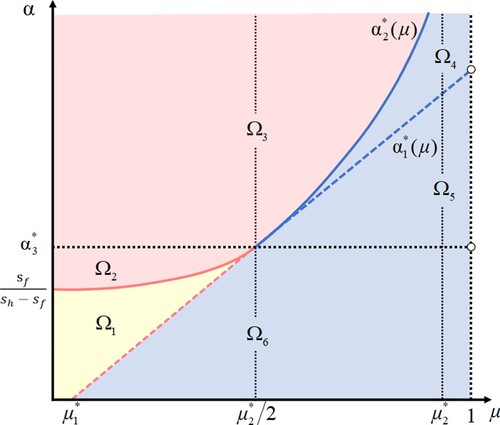
Figure 1. The division of the $\mu \alpha$-plane depending on the signs of $D(\mu ,\alpha )$, $f(0,\alpha )$ and ${\mathrm{\Gamma }}_x\left(\alpha \right)$. It shows that the curves ${\alpha }_1^{\ast }\left(\mu \right)$, ${\alpha }_2^{\ast }\left(\mu \right)$ and ${\alpha }_3^{\ast }$ divide the $\mu \alpha$-plane into six subregions: ${\mathrm{\Omega }}_1=\left\{\right(\mu ,\alpha ):D(\mu ,\alpha )>0,f(0,\alpha )>0,{\mathrm{\Gamma }}_x(\alpha )>0\}$, ${\mathrm{\Omega }}_2=\left\{\right(\mu ,\alpha ):D(\mu ,\alpha )>0,f(0,\alpha )<0,{\mathrm{\Gamma }}_x(\alpha )>0\}$, ${\mathrm{\Omega }}_3=\left\{\right(\mu ,\alpha ):D(\mu ,\alpha )>0,f(0,\alpha )<0,{\mathrm{\Gamma }}_x(\alpha )<0\}$, ${\mathrm{\Omega }}_4=\left\{\right(\mu ,\alpha ):D(\mu ,\alpha )>0,f(0,\alpha )>0,{\mathrm{\Gamma }}_x(\alpha )<0\}$, ${\mathrm{\Omega }}_5=\left\{\right(\mu ,\alpha ):D(\mu ,\alpha )<0,f(0,\alpha )>0,{\mathrm{\Gamma }}_x(\alpha )<0\}$ and ${\mathrm{\Omega }}_6=\left\{\right(\mu ,\alpha ):D(\mu ,\alpha )<0,f(0,\alpha )>0,{\mathrm{\Gamma }}_x(\alpha )>0\}$. There exist two positive equilibria in subregion ${\mathrm{\Omega }}_1$ (yellow), a unique positive equilibrium in subregions ${\mathrm{\Omega }}_2\cup {\mathrm{\Omega }}_3$ and two curves $\alpha ={\alpha }_2^{\ast }\left(\mu \right)$ for $\mu \in (0,{\mu }_2^{\ast }/2)$, and $\alpha ={\alpha }_1^{\ast }\left(\mu \right)$ for $\mu \in ({\mu }_1^{\ast },{\mu }_2^{\ast }/2)$ (red), and no positive equilibria in subregions ${\mathrm{\Omega }}_4\cup {\mathrm{\Omega }}_5\cup {\mathrm{\Omega }}_6$ together with the curve $\alpha ={\alpha }_2^{\ast }\left(\mu \right)$ for $\mu \in [{\mu }_2^{\ast }/2,{\mu }_2^{\ast })$ (blue).

Theorem 2.1

(1)	Model (4(4) $x_{n+1}=\frac{(1-\mu )(1-s_f)(1+\alpha )x_n}{s_h{x}_n^2-[s_f+s_h+\alpha (s_f-s_h\left)\right]x_n+1+\alpha (1-s_h)},n=0,1,2,\dots .$(4) ) has two positive equilibria: $\begin{array}{rl}{x}_1^{\ast }(\mu ,\alpha )& =\frac{s_h+s_f-\alpha (s_h-s_f)-\sqrt{D(\mu ,\alpha )}}{2s_h},\\ x_2^{\ast }(\mu ,\alpha )& =\frac{s_h+s_f-\alpha (s_h-s_f)+\sqrt{D(\mu ,\alpha )}}{2s_h}\end{array}$if and only if either $\mu \in (0,{\mu }_1^{\ast }]$ and $\alpha \in (0,{\alpha }_2^{\ast }(\mu \left)\right),$ or $\mu \in ({\mu }_1^{\ast },{\mu }_2^{\ast }/2)$ and $\alpha \in \left({\alpha }_1^{\ast }\right(\mu ),{\alpha }_2^{\ast }(\mu \left)\right)$ holds.
(2)	Model (4(4) $x_{n+1}=\frac{(1-\mu )(1-s_f)(1+\alpha )x_n}{s_h{x}_n^2-[s_f+s_h+\alpha (s_f-s_h\left)\right]x_n+1+\alpha (1-s_h)},n=0,1,2,\dots .$(4) ) has a unique positive equilibrium if one of the next two conditions holds. (i) $x_2^{\ast }(\mu ,\alpha )$ when $\mu \in (0,{\mu }_2^{\ast }/2)$ and $\alpha \ge {\alpha }_2^{\ast }\left(\mu \right),$ or $\mu \in ({\mu }_2^{\ast }/2,{\mu }_2^{\ast })$ and $\alpha >{\alpha }_2^{\ast }\left(\mu \right)$. (ii) $x^{\ast }(\mu ,{\alpha }_1^{\ast }(\mu \left)\right)=\frac{s_h+s_f-{\alpha }_1^{\ast }\left(\mu \right)(s_h-s_f)}{2s_h}=\frac{s_h-s_f-2\mu (1-s_f)}{s_h-s_f}$ for $\mu \in ({\mu }_1^{\ast },{\mu }_2^{\ast }/2)$.
(3)	Model (4(4) $x_{n+1}=\frac{(1-\mu )(1-s_f)(1+\alpha )x_n}{s_h{x}_n^2-[s_f+s_h+\alpha (s_f-s_h\left)\right]x_n+1+\alpha (1-s_h)},n=0,1,2,\dots .$(4) ) has no positive equilibria if and only if one of the following four conditions holds. (6) $\begin{array}{rl}\left(i\right)& \mu \in ({\mu }_1^{\ast },1)and\alpha \in (0,{\alpha }_1^{\ast }(\mu \left)\right).\end{array}$(6) (7) $\begin{array}{rl}\left(ii\right)& \mu \in [{\mu }_2^{\ast }/2,1)and\alpha ={\alpha }_1^{\ast }\left(\mu \right).\end{array}$(7) (8) $\begin{array}{rl}\left(iii\right)& \mu \in [{\mu }_2^{\ast }/2,{\mu }_2^{\ast })and\alpha \in \left({\alpha }_1^{\ast }\right(\mu ),{\alpha }_2^{\ast }(\mu \left)\right].\end{array}$(8) (9) $\begin{array}{rl}\left(iv\right)& \mu \in [{\mu }_2^{\ast },1)and\alpha >{\alpha }_1^{\ast }\left(\mu \right).\end{array}$(9)

2.3. Stability analysis

Before we explore the stability of the nonegative equilibria of model (4(4) $x_{n+1}=\frac{(1-\mu )(1-s_f)(1+\alpha )x_n}{s_h{x}_n^2-[s_f+s_h+\alpha (s_f-s_h\left)\right]x_n+1+\alpha (1-s_h)},n=0,1,2,\dots .$(4) ), define $G(x,\alpha )=\frac{a_{1}x}{s_h{x}^2-b_{1}x+c_1},$where $a_1=(1-\mu )(1-s_f)(1+\alpha ),b_1=s_f+s_h+\alpha (s_f-s_h),c_1=1+\alpha (1-s_h).$Then (4(4) $x_{n+1}=\frac{(1-\mu )(1-s_f)(1+\alpha )x_n}{s_h{x}_n^2-[s_f+s_h+\alpha (s_f-s_h\left)\right]x_n+1+\alpha (1-s_h)},n=0,1,2,\dots .$(4) ) becomes $x_{n+1}=G(x_n,\alpha )$. Taking the derivative of $G(x,\alpha )$ with respect to $x\in (0,1)$, we get (10) $\begin{array}{rl}\frac{\mathrm{\partial }G(x,\alpha )}{\mathrm{\partial }x}& =\frac{a_1(s_h{x}^2-b_{1}x+c_1)-a_{1}x(2s_{h}x-b_1)}{(s_h{x}^2-b_{1}x+c_1{)}^2}\\ & =\frac{a_1\left[\alpha \right(1-s_h)+(1-s_h{x}^2\left)\right]}{(s_h{x}^2-b_{1}x+c_1{)}^2}>0,\end{array}$(10) which implies that $G(x,\alpha )$ is strictly increasing with respect to $x\in (0,1)$. We see that equilibria $x_i^{\ast }(\mu ,\alpha )$, i = 1, 2, and $x^{\ast }(\mu ,{\alpha }_1^{\ast }(\mu \left)\right)$ satisfy $s_h{x}^2-b_{1}x+c_1-a_1=0.$Then the derivatives of $G(x,\alpha )$ at $x^{\ast }(\mu ,{\alpha }_1^{\ast }(\mu \left)\right)$ and $x_i^{\ast }(\mu ,\alpha )$, i = 1, 2 satisfy (11) $\frac{\mathrm{\partial }G(x,\alpha )}{\mathrm{\partial }x}=1-\frac{x(2s_{h}x-b_1)}{a_1}=1\pm \frac{x\sqrt{D(\mu ,\alpha )}}{a_1},$(11) which will be used to prove the stability of the positive equilibria of model (4(4) $x_{n+1}=\frac{(1-\mu )(1-s_f)(1+\alpha )x_n}{s_h{x}_n^2-[s_f+s_h+\alpha (s_f-s_h\left)\right]x_n+1+\alpha (1-s_h)},n=0,1,2,\dots .$(4) ).

Theorem 2.2

If either $\mu \in (0,{\mu }_1^{\ast }]$ and $\alpha \in (0,{\alpha }_2^{\ast }(\mu \left)\right),$ or $\mu \in ({\mu }_1^{\ast },{\mu }_2^{\ast }/2)$ and $\alpha \in \left({\alpha }_1^{\ast }\right(\mu ),{\alpha }_2^{\ast }(\mu \left)\right),$ then both the origin $x_0^{\ast }$ and $x_2^{\ast }(\mu ,\alpha )$ are locally asymptotically stable, while $x_1^{\ast }(\mu ,\alpha )$ is unstable.

Proof.

We first show that $x_0^{\ast }$ is locally asymptotically stable. In fact, since $\alpha <{\alpha }_2^{\ast }\left(\mu \right)$, we have $a_1=(1-\mu )(1-s_f)(1+\alpha )<1+\alpha (1-s_h)=c_1,$which leads to $0<\frac{\mathrm{\partial }G(x,\alpha )}{\mathrm{\partial }x}{|}_{x=x_0^{\ast }}=\frac{a_1}{c_1}<1.$Hence, from [1,9], the origin $x_0^{\ast }$ is locally asymptotically stable.

The local asymptotical stability of $x_2^{\ast }(\mu ,\alpha )$ can be obtained from (12) $\frac{\mathrm{\partial }G(x,\alpha )}{\mathrm{\partial }x}{|}_{x=x_2^{\ast }(\mu ,\alpha )}=1-\frac{x_2^{\ast }(\mu ,\alpha )\sqrt{D(\mu ,\alpha )}}{a_1}<1.$(12) Meanwhile, $\frac{\mathrm{\partial }G(x,\alpha )}{\mathrm{\partial }x}{|}_{x=x_1^{\ast }(\mu ,\alpha )}=1+\frac{x_1^{\ast }(\mu ,\alpha )\sqrt{D(\mu ,\alpha )}}{a_1}>1$implies the instability of $x_1^{\ast }(\mu ,\alpha )$. This completes the proof.

Theorem 2.3

The following two statements are true.

(1)	If either $\mu \in (0,{\mu }_2^{\ast }/2)$ and $\alpha \ge {\alpha }_2^{\ast }\left(\mu \right),$ or $\mu \in ({\mu }_2^{\ast }/2,{\mu }_2^{\ast })$ and $\alpha >{\alpha }_2^{\ast }\left(\mu \right)$, then the unique positive equilibrium $x_2^{\ast }(\mu ,\alpha )$ is globally asymptotically stable.
(2)	If $\mu \in ({\mu }_1^{\ast },{\mu }_2^{\ast }/2),$ then the origin $x_0^{\ast }$ is locally asymptotically stable and the unique positive equilibrium $x^{\ast }(\mu ,{\alpha }_1^{\ast }(\mu \left)\right)$ is semi-stable from the right side.

Proof.

(1) The local asymptotical stability of $x_2^{\ast }(\mu ,\alpha )$ is still guaranteed by (10(10) $\begin{array}{rl}\frac{\mathrm{\partial }G(x,\alpha )}{\mathrm{\partial }x}& =\frac{a_1(s_h{x}^2-b_{1}x+c_1)-a_{1}x(2s_{h}x-b_1)}{(s_h{x}^2-b_{1}x+c_1{)}^2}\\ & =\frac{a_1\left[\alpha \right(1-s_h)+(1-s_h{x}^2\left)\right]}{(s_h{x}^2-b_{1}x+c_1{)}^2}>0,\end{array}$(10) ) and (12(12) $\frac{\mathrm{\partial }G(x,\alpha )}{\mathrm{\partial }x}{|}_{x=x_2^{\ast }(\mu ,\alpha )}=1-\frac{x_2^{\ast }(\mu ,\alpha )\sqrt{D(\mu ,\alpha )}}{a_1}<1.$(12) ). To prove the global asymptotical stability of $x_2^{\ast }(\mu ,\alpha )$, we need to show that for any solution of model (4(4) $x_{n+1}=\frac{(1-\mu )(1-s_f)(1+\alpha )x_n}{s_h{x}_n^2-[s_f+s_h+\alpha (s_f-s_h\left)\right]x_n+1+\alpha (1-s_h)},n=0,1,2,\dots .$(4) ) initiated from $x_0\in (0,1)$, denoted by $\{x_n{\}}_{n=0}^{\mathrm{\infty }}=\{x_n(0,x_0){\}}_{n=0}^{\mathrm{\infty }}$, satisfies (13) $\underset{n\to \mathrm{\infty }}{lim}{x}_n=x_2^{\ast }(\mu ,\alpha ).$(13) Since $x_1^{\ast }(\mu ,\alpha )<0$ for $\mu \in (0,{\mu }_2^{\ast }/2)$ and $\alpha \ge {\alpha }_2^{\ast }\left(\mu \right)$, or $\mu \in ({\mu }_2^{\ast }/2,{\mu }_2^{\ast })$ and $\alpha >{\alpha }_2^{\ast }\left(\mu \right)$, from model (4(4) $x_{n+1}=\frac{(1-\mu )(1-s_f)(1+\alpha )x_n}{s_h{x}_n^2-[s_f+s_h+\alpha (s_f-s_h\left)\right]x_n+1+\alpha (1-s_h)},n=0,1,2,\dots .$(4) ), we have (14) $\mathrm{\Delta }{x}_n=x_{n+1}-x_n=-\frac{s_h{x}_n(x_n-x_1^{\ast }(\mu ,\alpha \left)\right)}{s_h{x}_n^2-b_1{x}_n+c_1}\cdot (x_n-x_2^{\ast }(\mu ,\alpha \left)\right),$(14) which further yields $x_{n+1}-x_2^{\ast }(\mu ,\alpha )=\mathrm{\Delta }{x}_n+x_n-x_2^{\ast }(\mu ,\alpha )=\frac{-(b_1-s_h{x}_1^{\ast }(\mu ,\alpha \left)\right)x_n+c_1}{s_h{x}_n^2-b_1{x}_n+c_1}\cdot (x_n-x_2^{\ast }(\mu ,\alpha \left)\right).$Since $y\left(x\right)=-(b_1-s_h{x}_1^{\ast }(\mu ,\alpha \left)\right)x+c_1$ is strictly decreasing in x, and $\begin{array}{rl}y\left(1\right)& =\frac{(1+\alpha )(2-s_f-s_h)-\sqrt{D(\mu ,\alpha )}}{2}\\ & >\frac{(1+\alpha )(2-s_f-s_h)-(1+\alpha )(s_h-s_f)}{2}\\ & =(1+\alpha )(1-s_h)>0\end{array}$from (5(5) $\begin{array}{rl}D(\mu ,\alpha )& =(1+\alpha )\left[\right(s_h-s_f{)}^2-4\mu s_h(1-s_f)+\alpha (s_h-s_f{)}^2]\\ & =(1+\alpha )\left[4s_h\right(1-s_f\left)\right({\mu }_1^{\ast }-\mu )+\alpha (s_h-s_f{)}^2]\\ & =(1+\alpha )(s_h-s_f{)}^2(\alpha -{\alpha }_1^{\ast }\left(\mu \right)),\end{array}$(5) ), we have $(x_{n+1}-x_2^{\ast }(\mu ,\alpha \left)\right)(x_n-x_2^{\ast }(\mu ,\alpha \left)\right)>0$ if $x_n\ne x_2^{\ast }(\mu ,\alpha )$. Equation (14(14) $\mathrm{\Delta }{x}_n=x_{n+1}-x_n=-\frac{s_h{x}_n(x_n-x_1^{\ast }(\mu ,\alpha \left)\right)}{s_h{x}_n^2-b_1{x}_n+c_1}\cdot (x_n-x_2^{\ast }(\mu ,\alpha \left)\right),$(14) ) implies that $\mathrm{\Delta }{x}_n>0$ for $x_0\in (0,x_2^{\ast }(\mu ,\alpha \left)\right)$, and $\mathrm{\Delta }{x}_n<0$ for $x_0\in \left(x_2^{\ast }\right(\mu ,\alpha ),1)$. Therefore, any solutions $\{x_n{\}}_{n=0}^{\mathrm{\infty }}$ of (4(4) $x_{n+1}=\frac{(1-\mu )(1-s_f)(1+\alpha )x_n}{s_h{x}_n^2-[s_f+s_h+\alpha (s_f-s_h\left)\right]x_n+1+\alpha (1-s_h)},n=0,1,2,\dots .$(4) ) initiated from $(0,x_2^{\ast }(\mu ,\alpha \left)\right)$ and $\left(x_2^{\ast }\right(\mu ,\alpha ),1)$ are monotonically increasing and decreasing, respectively. By letting $n\to \mathrm{\infty }$ in (4(4) $x_{n+1}=\frac{(1-\mu )(1-s_f)(1+\alpha )x_n}{s_h{x}_n^2-[s_f+s_h+\alpha (s_f-s_h\left)\right]x_n+1+\alpha (1-s_h)},n=0,1,2,\dots .$(4) ), we see that (13(13) $\underset{n\to \mathrm{\infty }}{lim}{x}_n=x_2^{\ast }(\mu ,\alpha ).$(13) ) holds.

(2) Since $\mu \in ({\mu }_1^{\ast },{\mu }_2^{\ast }/2)$, we have $D(\mu ,{\alpha }_1^{\ast }(\mu \left)\right)=0$. From (11(11) $\frac{\mathrm{\partial }G(x,\alpha )}{\mathrm{\partial }x}=1-\frac{x(2s_{h}x-b_1)}{a_1}=1\pm \frac{x\sqrt{D(\mu ,\alpha )}}{a_1},$(11) ), we have $\frac{\mathrm{\partial }G(x,\alpha )}{\mathrm{\partial }x}{|}_{x=x^{\ast }(\mu ,{\alpha }_1^{\ast }(\mu \left)\right)}=1$. The asymptotic stability criteria in [1,9] is not applicable. It follows from (4(4) $x_{n+1}=\frac{(1-\mu )(1-s_f)(1+\alpha )x_n}{s_h{x}_n^2-[s_f+s_h+\alpha (s_f-s_h\left)\right]x_n+1+\alpha (1-s_h)},n=0,1,2,\dots .$(4) ) that $\mathrm{\Delta }{x}_n=-\frac{s_h{x}_n(x_n-x^{\ast }(\mu ,{\alpha }_1^{\ast }\left(\mu \right)){)}^2}{s_h{x}_n^2-b_1{x}_n+c_1}<0\mathrm{f}\mathrm{o}\mathrm{r}\mathrm{a}\mathrm{n}\mathrm{y}{x}_n\ne x^{\ast }(\mu ,{\alpha }_1^{\ast }(\mu \left)\right).$Similar to the proof above, for any $x_0\in (0,x^{\ast }(\mu ,{\alpha }_1^{\ast }\left(\mu \right)\left)\right)$, solution $\{x_n{\}}_{n=0}^{\mathrm{\infty }}$ is monotonically decreasing, which proves the local asymptotical stability of the origin $x_0^{\ast }$, as well as the instability of $x^{\ast }(\mu ,{\alpha }_1^{\ast }(\mu \left)\right)$ from the left side. Meanwhile, the fact that $\{x_n{\}}_{n=0}^{\mathrm{\infty }}$ is monotonically decreasing for any $x_0\in \left(x^{\ast }\right(\mu ,{\alpha }_1^{\ast }\left(\mu \right)),1)$ ensures the stability of $x^{\ast }(\mu ,{\alpha }_1^{\ast }(\mu \left)\right)$ from the right side.

Theorem 2.4

The origin $x_0^{\ast }$ is globally asymptotically stable if one of (6(6) $\begin{array}{rl}\left(i\right)& \mu \in ({\mu }_1^{\ast },1)and\alpha \in (0,{\alpha }_1^{\ast }(\mu \left)\right).\end{array}$(6) )–(9(9) $\begin{array}{rl}\left(iv\right)& \mu \in [{\mu }_2^{\ast },1)and\alpha >{\alpha }_1^{\ast }\left(\mu \right).\end{array}$(9) ) holds.

Proof.

From the illustration on enumerating the positive equilibria of model (4(4) $x_{n+1}=\frac{(1-\mu )(1-s_f)(1+\alpha )x_n}{s_h{x}_n^2-[s_f+s_h+\alpha (s_f-s_h\left)\right]x_n+1+\alpha (1-s_h)},n=0,1,2,\dots .$(4) ) in Figure 1, to prove the global asymptotical stability of the origin $x_0^{\ast }$, we just need to prove that any solution $\{x_n{\}}_{n=0}^{\mathrm{\infty }}=\{x_n(0,x_0){\}}_{n=0}^{\mathrm{\infty }}$ of (4(4) $x_{n+1}=\frac{(1-\mu )(1-s_f)(1+\alpha )x_n}{s_h{x}_n^2-[s_f+s_h+\alpha (s_f-s_h\left)\right]x_n+1+\alpha (1-s_h)},n=0,1,2,\dots .$(4) ) is monotonically decreasing, where $x_0\in (0,1)$. From model (4(4) $x_{n+1}=\frac{(1-\mu )(1-s_f)(1+\alpha )x_n}{s_h{x}_n^2-[s_f+s_h+\alpha (s_f-s_h\left)\right]x_n+1+\alpha (1-s_h)},n=0,1,2,\dots .$(4) ), we find that we only need to show that (15) $f(x,\alpha )>0\text{ for all }x\in (0,1).$(15) In fact, we consider the next four possible cases, $\mu \in ({\mu }_1^{\ast },1)$, $\alpha \in (0,{\alpha }_1^{\ast }(\mu \left)\right)$, or $\mu \in [{\mu }_2^{\ast }/2,1)$, or $\mu \in [{\mu }_2^{\ast }/2,{\mu }_2^{\ast })$, $\alpha \in \left({\alpha }_1^{\ast }\right(\mu ),{\alpha }_2^{\ast }(\mu \left)\right]$, and or $\mu \in [{\mu }_2^{\ast },1)$, $\alpha >{\alpha }_1^{\ast }\left(\mu \right)$.

For the case when $\mu \in ({\mu }_1^{\ast },1)$ and $\alpha \in (0,{\alpha }_1^{\ast }(\mu \left)\right)$, we have $D(\mu ,\alpha )<0$. Since $f(0,\alpha )>0$ and $f(x,\alpha )$ has no zeros for $x\in (0,1)$, we see that (15(15) $f(x,\alpha )>0\text{ for all }x\in (0,1).$(15) ) holds.

For the case when $\mu \in [{\mu }_2^{\ast }/2,1)$, we get $D(\mu ,{\alpha }_1^{\ast }(\mu \left)\right)=0$. Then $f(0,{\alpha }_1^{\ast }(\mu \left)\right)\ge 0$ and ${\mathrm{\Gamma }}_x\left({\alpha }_1^{\ast }\right(\mu \left)\right)<0$ imply that $f(x,{\alpha }_1^{\ast }(\mu \left)\right)$ has no zeros for $x\in (0,1)$. Hence (15(15) $f(x,\alpha )>0\text{ for all }x\in (0,1).$(15) ) holds.

For the case when $\mu \in [{\mu }_2^{\ast }/2,{\mu }_2^{\ast })$ and $\alpha \in \left({\alpha }_1^{\ast }\right(\mu ),{\alpha }_2^{\ast }(\mu \left)\right]$, or $\mu \in [{\mu }_2^{\ast },1)$ and $\alpha >{\alpha }_1^{\ast }\left(\mu \right)$, we obtain $D(\mu ,\alpha )>0$. Together with $f(0,\alpha )>0$ and ${\mathrm{\Gamma }}_x\left(\alpha \right)<0$, we find that (15(15) $f(x,\alpha )>0\text{ for all }x\in (0,1).$(15) ) is also true. This completes the proof.

3. Releasing infected females with a constant ratio β

Population replacement aims to replace a local mosquito population with Wolbachia-infected ones so that their capacity in transmitting disease is reduced, whose implementation requires the release of infected females. For this purpose, we formulate the second discrete model and then analyse its dynamics.

3.1. Model formulation

When supplemental infected females are released with a constant ratio β to the total number of male/female mosquitoes $T_n=I_n^M+U_n^M(=I_n^F+U_n^F)$, the infection frequency of males is still $x_n$, while the infection frequency of females increases from $x_n$ to $\frac{I_n^F+\text{β}{T}_n}{T_n+\text{β}{T}_n}=\frac{x_n+\text{β}}{1+\text{β}}.$The proportion of infected mosquitoes at the $(n+1)$th generation is $P_{n+1}^I=(1-\mu )(1-s_f)\frac{x_n+\text{β}}{1+\text{β}},$since $P_{n+1}^I$ does not depend on the parental infection status. On $P_{n+1}^U$, taking the imperfect maternal transmission and incomplete CI into consideration, we have $P_{n+1}^U=\mu (1-s_f)\frac{x_n+\text{β}}{1+\text{β}}+(1-s_h)x_n\frac{1-x_n}{1+\text{β}}+\frac{(1-x_n{)}^2}{1+\text{β}},$where $\mu (1-s_f)(x_n+\text{β})/(1+\text{β})$ counts the proportion from infected females owing to maternal leakage, $(1-s_h)x_n(1-x_n)/(1+\text{β})$ is the proportion survived from CI, and $(1-x_n{)}^2/(1+\text{β})$ represents the proportion from uninfected matings. Therefore, the second discrete model in this paper is expressed as (16) $x_{n+1}=\frac{(1-\mu )(1-s_f)(\text{β}+x_n)}{s_h{x}_n^2-(s_f+s_h)x_n+1+\text{β}(1-s_f)},n=0,1,2,\dots .$(16)

3.2. Existence of equilibria

For model (16(16) $x_{n+1}=\frac{(1-\mu )(1-s_f)(\text{β}+x_n)}{s_h{x}_n^2-(s_f+s_h)x_n+1+\text{β}(1-s_f)},n=0,1,2,\dots .$(16) ), a positive equilibrium lying in $[0,1)$ satisfies $g(x,\text{β})=s_h{x}^3-(s_f+s_h)x^2+[s_f+(1-s_f\left)\right(\mu +\text{β}\left)\right]x-(1-\mu )(1-s_f)\text{β}=0.$We now investigate the zeros of $g(x,\text{β})=0$ in $[0,1)$. For any $\text{β}>0$, we get $g(0,\text{β})=-(1-\mu )(1-s_f)\text{β}<0\mathrm{a}\mathrm{n}\mathrm{d}g(1,\text{β})=\mu (1-s_f)(1+\text{β})>0,$which imply that equation $g(x,\text{β})=0$ has at least one solution in $(0,1)$, i.e.

Lemma 3.1

Model (16(16) $x_{n+1}=\frac{(1-\mu )(1-s_f)(\text{β}+x_n)}{s_h{x}_n^2-(s_f+s_h)x_n+1+\text{β}(1-s_f)},n=0,1,2,\dots .$(16) ) has at least one equilibrium in $(0,1)$.

To determine the number of the solutions of equation $g(x,\text{β})=0$ lying in $(0,1)$, we explore the monotonicity of function $g(x,\text{β})$ with respect to β. It follows from $g_{\text{β}}^{\prime }(x,\text{β})=(1-s_f)[x-(1-\mu \left)\right]$that $g(x,\text{β})$ is strictly decreasing with respect to β for $x<1-\mu$. Let $x_3^{\ast }(\mu ,\text{β})$ be the largest positive equilibrium of model (16(16) $x_{n+1}=\frac{(1-\mu )(1-s_f)(\text{β}+x_n)}{s_h{x}_n^2-(s_f+s_h)x_n+1+\text{β}(1-s_f)},n=0,1,2,\dots .$(16) ) lying in $(0,1)$, we claim that (17) $x_3^{\ast }(\mu ,\text{β})<1-\mu \text{ for }\text{β}\ge 0.$(17) In fact, let $H(x,\text{β})=\frac{(1-\mu )(1-s_f)(\text{β}+x)}{s_h{x}^2-(s_f+s_h)x+1+\text{β}(1-s_f)}.$Taking the derivative of $H(x,\text{β})$ with respect to $x\in (0,1)$, we have $\frac{\mathrm{\partial }H(x,\text{β})}{\mathrm{\partial }x}=(1-\mu )(1-s_f)\frac{1-s_h{x}^2+\text{β}[1-s_{h}x+s_h(1-x\left)\right]}{[s_h{x}^2-(s_f+s_h)x+1+\text{β}(1-s_f){]}^2}>0,$which implies that $H(x,\text{β})$ is strictly increasing with respect to $x\in (0,1)$. Hence, $x_3^{\ast }\left(\text{β}\right)=H\left(x_3^{\ast }\right(\text{β}),\text{β})<H(1,\text{β})=1-\mu$ for $\text{β}\ge 0$ and (17(17) $x_3^{\ast }(\mu ,\text{β})<1-\mu \text{ for }\text{β}\ge 0.$(17) ) holds. To sum up, we get

Lemma 3.2

Let $x_3^{\ast }(\mu ,\text{β})<1-\mu$ be the largest positive equilibrium of model (16(16) $x_{n+1}=\frac{(1-\mu )(1-s_f)(\text{β}+x_n)}{s_h{x}_n^2-(s_f+s_h)x_n+1+\text{β}(1-s_f)},n=0,1,2,\dots .$(16) ) lying in $(0,1)$. Then function $g(x,\text{β})$ is strictly decreasing with respect to β for $x<x_3^{\ast }(\mu ,\text{β})$.

Particularly, since $\begin{array}{rl}g(x,0)& =x[s_h{x}^2-(s_f+s_h)x+s_f+\mu (1-s_f\left)\right]\\ & =s_{h}x\left[{\left(x-\frac{s_f+s_h}{2s_h}\right)}^2+\frac{4s_h\mu (1-s_f)-(s_h-s_f{)}^2}{4s_h^2}\right]\\ & =s_{h}x\left[{\left(x-\frac{s_f+s_h}{2s_h}\right)}^2+\frac{4s_h(1-s_f)(\mu -{\mu }_1^{\ast })}{4s_h^2}\right],\end{array}$there are three possible cases to consider.

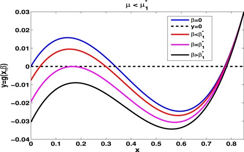
3.2.1. The case when $\mu \in (0,{\mu }_1^{\ast })$

For the case when $\mu \in (0,{\mu }_1^{\ast })$, function $g(x,0)$ has three zeros lying in $[0,1)$: $x_0^{\ast }=0,x_1^{\ast }\left(\mu \right)=\frac{s_h+s_f-\sqrt{D\left(\mu \right)}}{2s_h},\mathrm{a}\mathrm{n}\mathrm{d}{x}_2^{\ast }\left(\mu \right)=\frac{s_h+s_f-\sqrt{D\left(\mu \right)}}{2s_h},$where $D\left(\mu \right)$ is defined in Theorem 1.1 and positive. From Lemma 3.2, there exists a unique ${\text{β}}_1^{\ast }$ (see Figure 2 for illustration) such that

Figure 2. Given $s_f=0.1$ and $s_h=0.9$, we have ${\mu }_1^{\ast }\approx 0.1975$. For the case $\mu =0.15<{\mu }_1^{\ast }$, we get $x_1^{\ast }\left(\mu \right)\approx 0.3375$, $x_2^{\ast }\left(\mu \right)\approx 0.7736$. Numerical trials imply that ${\text{β}}_1^{\ast }\approx 0.0255$. Taking $\text{β}=0.01<{\text{β}}_1^{\ast }$, we have $x_1^{\ast }(\mu ,\text{β})\approx 0.0367$, $x_2^{\ast }(\mu ,\text{β})\approx 0.2987$ and $x_3^{\ast }(\mu ,\text{β})\approx 0.7758$. At ${\text{β}}_1^{\ast }$, $x_1^{\ast }(\mu ,{\text{β}}_1^{\ast })=x_2^{\ast }(\mu ,{\text{β}}_1^{\ast })\approx 0.1661$ and $x_3^{\ast }(\mu ,{\text{β}}_1^{\ast })\approx 0.7788$. Furthermore, when increasing β to 0.004, both $x_1^{\ast }(\mu ,\text{β})$ and $x_2^{\ast }(\mu ,\text{β})$ vanish, and $x_3^{\ast }(\mu ,\text{β})\approx 0.7815$.

Theorem 3.1

On enumerating the positive equilibria of model (16(16) $x_{n+1}=\frac{(1-\mu )(1-s_f)(\text{β}+x_n)}{s_h{x}_n^2-(s_f+s_h)x_n+1+\text{β}(1-s_f)},n=0,1,2,\dots .$(16) ) for $\mu \in (0,{\mu }_1^{\ast }),$ we have

(1)	If $\text{β}\in (0,{\text{β}}_1^{\ast }),$ then model (16(16) $x_{n+1}=\frac{(1-\mu )(1-s_f)(\text{β}+x_n)}{s_h{x}_n^2-(s_f+s_h)x_n+1+\text{β}(1-s_f)},n=0,1,2,\dots .$(16) ) admits three positive equilibria, denoted by $x_1^{\ast }(\mu ,\text{β}),$ $x_2^{\ast }(\mu ,\text{β})$ and $x_3^{\ast }(\mu ,\text{β})$. Furthermore, we have $0<x_1^{\ast }(\mu ,\text{β})<x_2^{\ast }(\mu ,\text{β})<x_1^{\ast }\left(\mu \right)<x_2^{\ast }\left(\mu \right)<x_3^{\ast }(\mu ,\text{β})<1-\mu .$
(2)	If $\text{β}={\text{β}}_1^{\ast },$ then model (16(16) $x_{n+1}=\frac{(1-\mu )(1-s_f)(\text{β}+x_n)}{s_h{x}_n^2-(s_f+s_h)x_n+1+\text{β}(1-s_f)},n=0,1,2,\dots .$(16) ) admits two positive equilibria $x_1^{\ast }(\mu ,{\text{β}}_1^{\ast })=x_2^{\ast }(\mu ,{\text{β}}_1^{\ast })$ and $x_3^{\ast }(\mu ,{\text{β}}_1^{\ast }).$
(3)	If $\text{β}>{\text{β}}_1^{\ast },$ then model (16(16) $x_{n+1}=\frac{(1-\mu )(1-s_f)(\text{β}+x_n)}{s_h{x}_n^2-(s_f+s_h)x_n+1+\text{β}(1-s_f)},n=0,1,2,\dots .$(16) ) admits a unique positive equilibrium $x_3^{\ast }(\mu ,\text{β})$.

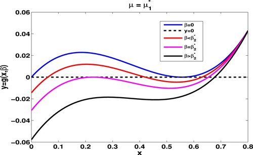
3.2.2. The case when $\mu ={\mu }_1^{\ast }$

For the case when $\mu ={\mu }_1^{\ast }$, function $g(x,0)$ has two zeros lying in $[0,1)$ which are $x_0^{\ast }=0,x_1^{\ast }\left({\mu }_1^{\ast }\right)=x_2^{\ast }\left({\mu }_1^{\ast }\right)=\frac{s_h+s_f}{2s_h}.$Again, from Lemma 3.2, there exists a unique ${\text{β}}_2^{\ast }$ (see Figure 3 for illustration) such that

Figure 3. Given $s_f=0.1$ and $s_h=0.9$, we take $\mu ={\mu }_1^{\ast }\approx 0.1975$. When $\text{β}=0$, $x_1^{\ast }\left({\mu }_1^{\ast }\right)$ and $x_2^{\ast }\left({\mu }_1^{\ast }\right)$ coincide to $x_1^{\ast }\left({\mu }_1^{\ast }\right)=x_2^{\ast }\left({\mu }_1^{\ast }\right)\approx 0.5556$. Numerical trials offer ${\text{β}}_2^{\ast }\approx 0.0426$. When $\text{β}=0.02<{\text{β}}_2^{\ast }$, $x_1^{\ast }({\mu }_1^{\ast },\text{β})\approx 0.0606$, $x_2^{\ast }({\mu }_1^{\ast },\text{β})\approx 0.4209$ and $x_3^{\ast }({\mu }_1^{\ast },\text{β})\approx 0.6296$. When $\text{β}={\text{β}}_2^{\ast }$, both $x_1^{\ast }({\mu }_1^{\ast },{\text{β}}_2^{\ast })$ and $x_2^{\ast }({\mu }_1^{\ast },{\text{β}}_2^{\ast })$ coincide to $x_1^{\ast }({\mu }_1^{\ast },{\text{β}}_2^{\ast })=x_2^{\ast }({\mu }_1^{\ast },{\text{β}}_2^{\ast })\approx 0.2280$ and $x_3^{\ast }({\mu }_1^{\ast },{\text{β}}_2^{\ast })\approx 0.6539$. For $\text{β}=0.08>{\text{β}}_2^{\ast }$, $x_3^{\ast }({\mu }_1^{\ast },\text{β})\approx 0.6772$.

Theorem 3.2

Assume that $\mu ={\mu }_1^{\ast }$. Then the following three statements are true.

(1)	If $\text{β}\in (0,{\text{β}}_2^{\ast })$, then model (16(16) $x_{n+1}=\frac{(1-\mu )(1-s_f)(\text{β}+x_n)}{s_h{x}_n^2-(s_f+s_h)x_n+1+\text{β}(1-s_f)},n=0,1,2,\dots .$(16) ) admits three positive equilibria $x_1^{\ast }({\mu }_1^{\ast },\text{β}),$ $x_2^{\ast }({\mu }_1^{\ast },\text{β})$ and $x_3^{\ast }({\mu }_1^{\ast },\text{β})$ with $0<x_1^{\ast }({\mu }_1^{\ast },\text{β})<x_2^{\ast }({\mu }_1^{\ast },\text{β})<x_1^{\ast }\left({\mu }_1^{\ast }\right)=x_2^{\ast }\left({\mu }_1^{\ast }\right)<x_3^{\ast }({\mu }_1^{\ast },\text{β})<1-{\mu }_1^{\ast }.$
(2)	If $\text{β}={\text{β}}_2^{\ast },$ then model (16(16) $x_{n+1}=\frac{(1-\mu )(1-s_f)(\text{β}+x_n)}{s_h{x}_n^2-(s_f+s_h)x_n+1+\text{β}(1-s_f)},n=0,1,2,\dots .$(16) ) admits two positive equilibria $x_1^{\ast }({\mu }_1^{\ast },{\text{β}}_2^{\ast })=x_2^{\ast }({\mu }_1^{\ast },{\text{β}}_2^{\ast })$ and $x_3^{\ast }({\mu }_1^{\ast },{\text{β}}_2^{\ast }).$
(3)	If $\text{β}>{\text{β}}_2^{\ast },$ then model (16(16) $x_{n+1}=\frac{(1-\mu )(1-s_f)(\text{β}+x_n)}{s_h{x}_n^2-(s_f+s_h)x_n+1+\text{β}(1-s_f)},n=0,1,2,\dots .$(16) ) admits a unique positive equilibrium $x_3^{\ast }({\mu }_1^{\ast },\text{β})$.

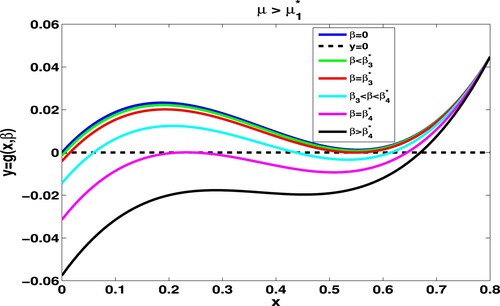
3.2.3. The case when $\mu >{\mu }_1^{\ast }$

For the case when $\mu >{\mu }_1^{\ast }$, we have $g(x,0)>0$ for $x\in (0,1)$. As β  increases, from Lemma 3.2, there exist ${\text{β}}_3^{\ast }$ and ${\text{β}}_4^{\ast }$ (see Figure 4 for illustration) such that

Figure 4. Given $s_f=0.1$ and $s_h=0.9$, we take $\mu =0.2>{\mu }_1^{\ast }\approx 0.1975$. Numerical simulations show that ${\text{β}}_3^{\ast }\approx 0.0057$, ${\text{β}}_4^{\ast }\approx 0.0437$. The number of zeros of $g(x,\text{β})$ lying in $(0,1)$ goes from 1, passing 2, 3, 2, and finally to 1 as β increases from 0 to the β with $\text{β}>{\text{β}}_4^{\ast }$.

Theorem 3.3

Assume that $\mu >{\mu }_1^{\ast }$. Then the following three statements are true.

(1)	If $\text{β}\in (0,{\text{β}}_3^{\ast })\cup ({\text{β}}_4^{\ast },+\mathrm{\infty })$, then model (16(16) $x_{n+1}=\frac{(1-\mu )(1-s_f)(\text{β}+x_n)}{s_h{x}_n^2-(s_f+s_h)x_n+1+\text{β}(1-s_f)},n=0,1,2,\dots .$(16) ) admits a unique positive equilibrium. The unique positive equilibrium is $x_1^{\ast }(\mu ,\text{β})$ for $\text{β}\in (0,{\text{β}}_3^{\ast }),$ or $x_3^{\ast }(\mu ,\text{β})$ for $\text{β}\in ({\text{β}}_4^{\ast },+\mathrm{\infty })$.
(2)	If $\text{β}={\text{β}}_3^{\ast }$ (or $\text{β}={\text{β}}_4^{\ast }$), then model (16(16) $x_{n+1}=\frac{(1-\mu )(1-s_f)(\text{β}+x_n)}{s_h{x}_n^2-(s_f+s_h)x_n+1+\text{β}(1-s_f)},n=0,1,2,\dots .$(16) ) admits two positive equilibria $x_1^{\ast }(\mu ,{\text{β}}_3^{\ast })=x_2^{\ast }(\mu ,{\text{β}}_3^{\ast })$, $x_3^{\ast }(\mu ,{\text{β}}_4^{\ast })$ (or $x_1^{\ast }(\mu ,\text{β}),$ $x_2^{\ast }(\mu ,{\text{β}}_4^{\ast })=x_3^{\ast }(\mu ,{\text{β}}_4^{\ast })$).
(3)	If $\text{β}\in ({\text{β}}_3^{\ast },{\text{β}}_4^{\ast })$, then model (16(16) $x_{n+1}=\frac{(1-\mu )(1-s_f)(\text{β}+x_n)}{s_h{x}_n^2-(s_f+s_h)x_n+1+\text{β}(1-s_f)},n=0,1,2,\dots .$(16) ) admits three positive equilibria $x_1^{\ast }(\mu ,\text{β}),$ $x_2^{\ast }(\mu ,\text{β})$ and $x_3^{\ast }(\mu ,\text{β})$ satisfying $\begin{array}{rl}& 0<x_1^{\ast }(\mu ,{\text{β}}_3^{\ast })<x_1^{\ast }(\mu ,\text{β})<x_1^{\ast }(\mu ,{\text{β}}_4^{\ast })=x_2^{\ast }(\mu ,{\text{β}}_4^{\ast })<x_2^{\ast }(\mu ,\text{β})\\ & <x_2^{\ast }(\mu ,{\text{β}}_3^{\ast })=x_3^{\ast }(\mu ,{\text{β}}_3^{\ast })<x_3^{\ast }(\mu ,\text{β})<x_3^{\ast }(\mu ,{\text{β}}_4^{\ast })<1-\mu .\end{array}$

3.3. Stability analysis

In this section, we investigate the stability of the positive equilibria of model (16(16) $x_{n+1}=\frac{(1-\mu )(1-s_f)(\text{β}+x_n)}{s_h{x}_n^2-(s_f+s_h)x_n+1+\text{β}(1-s_f)},n=0,1,2,\dots .$(16) ). The following first result generates a bistable dynamics for the case when there exist three positive equilibria.

Theorem 3.4

If $(\mu ,\text{β})\in \left\{\right(\mu ,\text{β}):0<\mu <{\mu }_1^{\ast },\text{β}\in (0,{\text{β}}_1^{\ast }\left)\right\}\cup \left\{\right(\mu ,\text{β}):\mu ={\mu }_1^{\ast },\text{β}\in (0,{\text{β}}_2^{\ast }\left)\right\}\cup \left\{\right(\mu ,\text{β}):\mu >{\mu }_1^{\ast },{\text{β}}_3^{\ast }<\text{β}<{\text{β}}_4^{\ast }\},$ then model (16(16) $x_{n+1}=\frac{(1-\mu )(1-s_f)(\text{β}+x_n)}{s_h{x}_n^2-(s_f+s_h)x_n+1+\text{β}(1-s_f)},n=0,1,2,\dots .$(16) ) has three positive equilibria $x_1^{\ast }(\mu ,\text{β})$, $x_2^{\ast }(\mu ,\text{β})$ and $x_3^{\ast }(\mu ,\text{β}),$ where both $x_1^{\ast }(\mu ,\text{β})$ and $x_3^{\ast }(\mu ,\text{β})$ are locally asymptotically stable, while $x_2^{\ast }(\mu ,\text{β})$ is unstable.

Proof.

We first show that $x_1^{\ast }(\mu ,\text{β})$ is locally asymptotically stable. For any initial value $x_0\in (0,x_1^{\ast }(\mu ,\text{β}\left)\right)$, from (16(16) $x_{n+1}=\frac{(1-\mu )(1-s_f)(\text{β}+x_n)}{s_h{x}_n^2-(s_f+s_h)x_n+1+\text{β}(1-s_f)},n=0,1,2,\dots .$(16) ), it is easy to see that $\mathrm{\Delta }{x}_0>0$ and hence $x_1>x_0$. Therefore, we reach $x_{n+1}>x_n$ by induction for all $n\ge 0$, which means that solution $\{x_n{\}}_{n=0}^{\mathrm{\infty }}$ monotonically increases to $x_1^{\ast }(\mu ,\text{β})$ if $x_0\in (0,x_1^{\ast }(\mu ,\text{β}\left)\right)$. Similarly, we can prove that any solutions initiated from $\left(x_1^{\ast }\right(\mu ,\text{β}),x_2^{\ast }(\mu ,\text{β}\left)\right)$ monotonically decrease to $x_1^{\ast }(\mu ,\text{β})$, and any solutions initiated from $\left(x_2^{\ast }\right(\mu ,\text{β}),x_3^{\ast }(\mu ,\text{β}\left)\right)$ (or $\left(x_3^{\ast }\right(\mu ,\text{β}),1)$) monotonically increase (or decrease) to $x_3^{\ast }(\mu ,\text{β})$. While the instability of $x_2^{\ast }(\mu ,\text{β})$ is obvious. The proof is finished.

For the case when $(\mu ,\text{β})\in \left\{\right(\mu ,\text{β}):0<\mu <{\mu }_1^{\ast },\text{β}={\text{β}}_1^{\ast }\}\cup \left\{\right(\mu ,\text{β}):\mu ={\mu }_1^{\ast },\text{β}={\text{β}}_2^{\ast }\}\cup \left\{\right(\mu ,\text{β}):\mu >{\mu }_1^{\ast },\text{β}={\text{β}}_4^{\ast }\}$, equilibria $x_1^{\ast }(\mu ,\text{β})$ and $x_2^{\ast }(\mu ,\text{β})$ shrink to one, which is semi-stable. While for $(\mu ,\text{β})\in \left\{\right(\mu ,\text{β}):\mu >{\mu }_1^{\ast },\text{β}={\text{β}}_3^{\ast }\}$, $x_2^{\ast }(\mu ,\text{β})$ and $x_3^{\ast }(\mu ,\text{β})$ coincide, which is also semi-stable. To sum up, we have

Theorem 3.5

The following two statements are true.

(1)

If $(\mu ,\text{β})\in \left\{\right(\mu ,\text{β}):0<\mu <{\mu }_1^{\ast },\text{β}={\text{β}}_1^{\ast }\}\cup \left\{\right(\mu ,\text{β}):\mu ={\mu }_1^{\ast },\text{β}={\text{β}}_2^{\ast }\}\cup \left\{\right(\mu ,\text{β}):\mu >{\mu }_1^{\ast },\text{β}={\text{β}}_4^{\ast }\},$ then $x_3^{\ast }(\mu ,\text{β})$ is locally asymptotically stable, and $x_1^{\ast }(\mu ,\text{β})=x_2^{\ast }(\mu ,\text{β})$ is semi-stable from the right side.

(2)

If $(\mu ,\text{β})\in \left\{\right(\mu ,\text{β}):\mu >{\mu }_1^{\ast },\text{β}={\text{β}}_3^{\ast }\}$, then $x_2^{\ast }(\mu ,\text{β})=x_3^{\ast }(\mu ,\text{β})$ is semi-stable from the left side, and $x_1^{\ast }(\mu ,\text{β})$ is locally asymptotically stable.

The following theorem indicates that the unique positive equilibrium is globally asymptotically stable.

Theorem 3.6

If $(\mu ,\text{β})\in \left\{\right(\mu ,\text{β}):0<\mu <{\mu }_1^{\ast },\text{β}>{\text{β}}_1^{\ast }\}\cup \left\{\right(\mu ,\text{β}):\mu ={\mu }_1^{\ast },\text{β}>{\text{β}}_2^{\ast }\}\cup \left\{\right(\mu ,\text{β}):\mu >{\mu }_1^{\ast },0<\text{β}<{\text{β}}_3^{\ast }\}\cup \left\{\right(\mu ,\text{β}):\mu >{\mu }_1^{\ast },\text{β}>{\text{β}}_4^{\ast }\},$ then the unique positive equilibrium is globally asymptotically stable.

4. Discussions

4.1. Dynamics driven by (4) and (16)

Two discrete models (4(4) $x_{n+1}=\frac{(1-\mu )(1-s_f)(1+\alpha )x_n}{s_h{x}_n^2-[s_f+s_h+\alpha (s_f-s_h\left)\right]x_n+1+\alpha (1-s_h)},n=0,1,2,\dots .$(4) ) and (16(16) $x_{n+1}=\frac{(1-\mu )(1-s_f)(\text{β}+x_n)}{s_h{x}_n^2-(s_f+s_h)x_n+1+\text{β}(1-s_f)},n=0,1,2,\dots .$(16) ) are formulated to study the dynamics of Wolbachia infection frequency in cage mosquito populations. Model (4(4) $x_{n+1}=\frac{(1-\mu )(1-s_f)(1+\alpha )x_n}{s_h{x}_n^2-[s_f+s_h+\alpha (s_f-s_h\left)\right]x_n+1+\alpha (1-s_h)},n=0,1,2,\dots .$(4) ) aims to the infection frequency when only infected males are released at every generation with a constant release ratio α. For given $s_f$ and $s_h$, enumeration of the positive equilibria of (4(4) $x_{n+1}=\frac{(1-\mu )(1-s_f)(1+\alpha )x_n}{s_h{x}_n^2-[s_f+s_h+\alpha (s_f-s_h\left)\right]x_n+1+\alpha (1-s_h)},n=0,1,2,\dots .$(4) ) is offered in Theorem 2.1, depending on the values of the maternal leakage rate μ and α relative to ${\mu }_1^{\ast }$, ${\mu }_2^{\ast }$, ${\alpha }_1^{\ast }\left(\mu \right)$ and ${\alpha }_2^{\ast }\left(\mu \right)$. Theorem 2.2 shows that (4(4) $x_{n+1}=\frac{(1-\mu )(1-s_f)(1+\alpha )x_n}{s_h{x}_n^2-[s_f+s_h+\alpha (s_f-s_h\left)\right]x_n+1+\alpha (1-s_h)},n=0,1,2,\dots .$(4) ) generates a bistable dynamics when there exist two positive equilibria. When the positive equilibrium is unique, Theorem 2.3 shows that it is either globally asymptotically stable or semi-stable. When there is no positive equilibria, Theorem 2.4 proves the global asymptotical stability of the origin $x_0^{\ast }$.

Regarding the situation when only infected females are supplementally released, model (16(16) $x_{n+1}=\frac{(1-\mu )(1-s_f)(\text{β}+x_n)}{s_h{x}_n^2-(s_f+s_h)x_n+1+\text{β}(1-s_f)},n=0,1,2,\dots .$(16) ) introduced the constant release ratio β. By using the maximal leakage rate ${\mu }_1^{\ast }$ deduced in [37]. The existence of the positive equilibria of model (16(16) $x_{n+1}=\frac{(1-\mu )(1-s_f)(\text{β}+x_n)}{s_h{x}_n^2-(s_f+s_h)x_n+1+\text{β}(1-s_f)},n=0,1,2,\dots .$(16) ) is characterized in Theorems 3.1–3.3, along the existence of four thresholds of β, denoted by ${\text{β}}_1^{\ast }$ in Theorem 3.1, ${\text{β}}_2^{\ast }$ in Theorem 3.2, as well as ${\text{β}}_3^{\ast }$ and ${\text{β}}_4^{\ast }$ with ${\text{β}}_3^{\ast }<{\text{β}}_4^{\ast }$ in Theorem 3.3. Different from model (4(4) $x_{n+1}=\frac{(1-\mu )(1-s_f)(1+\alpha )x_n}{s_h{x}_n^2-[s_f+s_h+\alpha (s_f-s_h\left)\right]x_n+1+\alpha (1-s_h)},n=0,1,2,\dots .$(4) ), model (16(16) $x_{n+1}=\frac{(1-\mu )(1-s_f)(\text{β}+x_n)}{s_h{x}_n^2-(s_f+s_h)x_n+1+\text{β}(1-s_f)},n=0,1,2,\dots .$(16) ) has no the origin $x_0^{\ast }$. Bistable dynamics occurs when there are three positive equilibria. Let $x_i^{\ast }(\mu ,\text{β})$, i = 1, 2, 3 satisfying $x_1^{\ast }(\mu ,\text{β})\le x_2^{\ast }(\mu ,\text{β})\le x_3^{\ast }(\mu ,\text{β})$ denote the three positive equilibria of (16(16) $x_{n+1}=\frac{(1-\mu )(1-s_f)(\text{β}+x_n)}{s_h{x}_n^2-(s_f+s_h)x_n+1+\text{β}(1-s_f)},n=0,1,2,\dots .$(16) ). Theorem 3.4 manifests that both $x_1^{\ast }(\mu ,\text{β})$ and $x_3^{\ast }(\mu ,\text{β})$ are locally asymptotically stable, while $x_2^{\ast }(\mu ,\text{β})$ is unstable. Theorem 3.5 shows that if $x_1^{\ast }(\mu ,\text{β})$ equals to $x_2^{\ast }(\mu ,\text{β})$ at $\text{β}={\text{β}}_i^{\ast }$, i = 1, 2, 4, then $x_1^{\ast }(\mu ,\text{β})=x_2^{\ast }(\mu ,\text{β})$ is semi-stable and $x_3^{\ast }(\mu ,\text{β})$ is locally asymptotically stable. Also, when $x_2^{\ast }(\mu ,\text{β})$ equals to $x_3^{\ast }(\mu ,\text{β})$ at $\text{β}={\text{β}}_3^{\ast }$, $x_1^{\ast }(\mu ,{\text{β}}_3^{\ast })$ is locally asymptotically stable and $x_2^{\ast }(\mu ,{\text{β}}_3^{\ast })=x_3^{\ast }(\mu ,{\text{β}}_3^{\ast })$ is semi-stable.

We take $s_f=0.1$ and $s_h=0.9$ as an example to illustrate our theoretical results. The parameters μ, α and β are chosen so that both models (4(4) $x_{n+1}=\frac{(1-\mu )(1-s_f)(1+\alpha )x_n}{s_h{x}_n^2-[s_f+s_h+\alpha (s_f-s_h\left)\right]x_n+1+\alpha (1-s_h)},n=0,1,2,\dots .$(4) ) and (16(16) $x_{n+1}=\frac{(1-\mu )(1-s_f)(\text{β}+x_n)}{s_h{x}_n^2-(s_f+s_h)x_n+1+\text{β}(1-s_f)},n=0,1,2,\dots .$(16) ) generate bistable dynamics. In this case, we have ${\mu }_1^{\ast }\approx 0.1975,{\alpha }_2^{\ast }\approx 0.3534,{\text{β}}_1^{\ast }\approx \mathrm{0.0073.}$From Theorems 2.1 and 3.1, when we take $\mu =0.15\in (0,{\mu }_1^{\ast })$, $\alpha =0.01\in (0,{\alpha }_2^{\ast })$, and $\text{β}=0.01\in (0,{\text{β}}_1^{\ast })$, both model (4(4) $x_{n+1}=\frac{(1-\mu )(1-s_f)(1+\alpha )x_n}{s_h{x}_n^2-[s_f+s_h+\alpha (s_f-s_h\left)\right]x_n+1+\alpha (1-s_h)},n=0,1,2,\dots .$(4) ) and model (16(16) $x_{n+1}=\frac{(1-\mu )(1-s_f)(\text{β}+x_n)}{s_h{x}_n^2-(s_f+s_h)x_n+1+\text{β}(1-s_f)},n=0,1,2,\dots .$(16) ) admit three equilibria in $[0,1)$, which are shown in Figure 5. Model (16(16) $x_{n+1}=\frac{(1-\mu )(1-s_f)(\text{β}+x_n)}{s_h{x}_n^2-(s_f+s_h)x_n+1+\text{β}(1-s_f)},n=0,1,2,\dots .$(16) ) generates a lower infection frequency threshold with $x_2^{\ast }(\mu ,\text{β})\approx 0.2987<0.3275\approx x_1^{\ast }(\mu ,\alpha )$, and a slightly higher polymorphic infection frequency with $x_3^{\ast }(\mu ,\text{β})\approx 0.7758>0.7747\approx x_2^{\ast }(\mu ,\alpha )$. This observation implies that releasing infected females is more efficient than releasing infected males at the same constant ratio.

Figure 5. Distable dynamics driven by model (4(4) $x_{n+1}=\frac{(1-\mu )(1-s_f)(1+\alpha )x_n}{s_h{x}_n^2-[s_f+s_h+\alpha (s_f-s_h\left)\right]x_n+1+\alpha (1-s_h)},n=0,1,2,\dots .$(4) ) and model (16(16) $x_{n+1}=\frac{(1-\mu )(1-s_f)(\text{β}+x_n)}{s_h{x}_n^2-(s_f+s_h)x_n+1+\text{β}(1-s_f)},n=0,1,2,\dots .$(16) ). Panel (A) is for model (4(4) $x_{n+1}=\frac{(1-\mu )(1-s_f)(1+\alpha )x_n}{s_h{x}_n^2-[s_f+s_h+\alpha (s_f-s_h\left)\right]x_n+1+\alpha (1-s_h)},n=0,1,2,\dots .$(4) ) and Panel (B) is for model (16(16) $x_{n+1}=\frac{(1-\mu )(1-s_f)(\text{β}+x_n)}{s_h{x}_n^2-(s_f+s_h)x_n+1+\text{β}(1-s_f)},n=0,1,2,\dots .$(16) ).

4.2. Comparisons on three release strategies introduced in (3), (4) and (16)

The above observation that model (16(16) $x_{n+1}=\frac{(1-\mu )(1-s_f)(\text{β}+x_n)}{s_h{x}_n^2-(s_f+s_h)x_n+1+\text{β}(1-s_f)},n=0,1,2,\dots .$(16) ) performs better than model (4(4) $x_{n+1}=\frac{(1-\mu )(1-s_f)(1+\alpha )x_n}{s_h{x}_n^2-[s_f+s_h+\alpha (s_f-s_h\left)\right]x_n+1+\alpha (1-s_h)},n=0,1,2,\dots .$(4) ) for $\mu =0.15$ and $\alpha =\text{β}=0.01$ is not a special case, but a general one. To see this, we plot the infection frequency thresholds driven by model (3(3) $\begin{array}{rl}{x}_{n+1}& =\frac{(1-\mu )(1-s_f)(1+r)(x_n+r)}{s_h{x}_n^2-\left[s_f+s_h+r(s_f-s_h)\right]x_n+1+(2-s_f-s_h)r+(1-s_f)r^2},\\ & n=0,1,2,\dots \end{array}$(3) ) with r = 0.0005, model (16(16) $x_{n+1}=\frac{(1-\mu )(1-s_f)(\text{β}+x_n)}{s_h{x}_n^2-(s_f+s_h)x_n+1+\text{β}(1-s_f)},n=0,1,2,\dots .$(16) ) with $\text{β}=0.0005$ and model (4(4) $x_{n+1}=\frac{(1-\mu )(1-s_f)(1+\alpha )x_n}{s_h{x}_n^2-[s_f+s_h+\alpha (s_f-s_h\left)\right]x_n+1+\alpha (1-s_h)},n=0,1,2,\dots .$(4) ) with $\alpha =0.0005$ for $\mu \in (0,{\mu }_1^{\ast })$, $s_f=0.1$ and $s_h=0.9$ in Figure 6(A), the infection frequency threshold generated from model (3(3) $\begin{array}{rl}{x}_{n+1}& =\frac{(1-\mu )(1-s_f)(1+r)(x_n+r)}{s_h{x}_n^2-\left[s_f+s_h+r(s_f-s_h)\right]x_n+1+(2-s_f-s_h)r+(1-s_f)r^2},\\ & n=0,1,2,\dots \end{array}$(3) ) is the smallest, while the release strategy with only infected males released requires the largest threshold for Wolbachia fixation. Meanwhile, Figure 6(B) plots the polymorphic states (the largest positive equilibria) for μ under the three release strategies driven by (3(3) $\begin{array}{rl}{x}_{n+1}& =\frac{(1-\mu )(1-s_f)(1+r)(x_n+r)}{s_h{x}_n^2-\left[s_f+s_h+r(s_f-s_h)\right]x_n+1+(2-s_f-s_h)r+(1-s_f)r^2},\\ & n=0,1,2,\dots \end{array}$(3) ), (16(16) $x_{n+1}=\frac{(1-\mu )(1-s_f)(\text{β}+x_n)}{s_h{x}_n^2-(s_f+s_h)x_n+1+\text{β}(1-s_f)},n=0,1,2,\dots .$(16) ) and (4(4) $x_{n+1}=\frac{(1-\mu )(1-s_f)(1+\alpha )x_n}{s_h{x}_n^2-[s_f+s_h+\alpha (s_f-s_h\left)\right]x_n+1+\alpha (1-s_h)},n=0,1,2,\dots .$(4) ), respectively. It shows that releasing both infected females and males brings the Wolbachia to fix at the highest infection level. And when only infected males are supplementally released, the Wolbachia infection frequency will fix at the lowest one. For the three release strategies, the increase of μ pulls the infection frequency thresholds higher, and drags down the Wolbachia fixation frequencies.

Figure 6. Comparisons on the infection frequency thresholds (A) and the polymorphic states (B) driven by (3(3) $\begin{array}{rl}{x}_{n+1}& =\frac{(1-\mu )(1-s_f)(1+r)(x_n+r)}{s_h{x}_n^2-\left[s_f+s_h+r(s_f-s_h)\right]x_n+1+(2-s_f-s_h)r+(1-s_f)r^2},\\ & n=0,1,2,\dots \end{array}$(3) ), (16(16) $x_{n+1}=\frac{(1-\mu )(1-s_f)(\text{β}+x_n)}{s_h{x}_n^2-(s_f+s_h)x_n+1+\text{β}(1-s_f)},n=0,1,2,\dots .$(16) ) and (4(4) $x_{n+1}=\frac{(1-\mu )(1-s_f)(1+\alpha )x_n}{s_h{x}_n^2-[s_f+s_h+\alpha (s_f-s_h\left)\right]x_n+1+\alpha (1-s_h)},n=0,1,2,\dots .$(4) ) on different maternal leakage rates μ lying in $(0,{\mu }_1^{\ast })$.

4.3. Implications on the design of release strategy

Regarding the Wolbachia persistence in cage experiments, the two most crucial concerns are: (1) how fast the persistence is when the initial infection frequency is larger than the infection frequency threshold. (2) how supplemental releases of infected mosquitoes lower the infection frequency threshold to make the persistence achievable. To answer such two questions numerically, let $s_f=0.1,s_h=0.9,\mu =\mathrm{0.05.}$Numerical trials indicate that ${\alpha }_2^{\ast }\approx 0.1921$ in Theorem 2.1, ${\text{β}}_1^{\ast }\approx 0.0073$ in Theorem 3.1, and $r^{\ast }\approx 0.00726$ in Theorem 3.1 in [37]. Take $\alpha =\text{β}=r=0.005$, we have $\begin{array}{rl}& x_1^{\ast }(\mu ,\alpha )\approx 0.1670,x_2^{\ast }(\mu ,\text{β})\approx 0.1335,x_2^{\ast }(\mu ,r)\approx 0.1347,\\ & x_2^{\ast }(\mu ,\alpha )\approx 0.9397,x_3^{\ast }(\mu ,\text{β})\approx 0.9397,x_3^{\ast }(\mu ,r)\approx \mathrm{0.9340.}\end{array}$Hence, if we define $\begin{array}{rl}{x}_2^{\ast \ast }& =max\left\{x_1^{\ast }\right(\mu ,\alpha ),x_2^{\ast }(\mu ,\text{β}),x_2^{\ast }(\mu ,r\left)\right\}\approx 0.1670,\\ x_3^{\ast \ast }& =min\left\{x_2^{\ast }\right(\mu ,\alpha ),x_3^{\ast }(\mu ,\text{β}),x_3^{\ast }(\mu ,r\left)\right\}\approx 0.9340,\end{array}$then solutions initiated from $(0.18,0.92)\in (x_2^{\ast \ast },x_3^{\ast \ast })$ will eventually go to Wolbachia fixation under three release strategies modelled by (3(3) $\begin{array}{rl}{x}_{n+1}& =\frac{(1-\mu )(1-s_f)(1+r)(x_n+r)}{s_h{x}_n^2-\left[s_f+s_h+r(s_f-s_h)\right]x_n+1+(2-s_f-s_h)r+(1-s_f)r^2},\\ & n=0,1,2,\dots \end{array}$(3) ), (16(16) $x_{n+1}=\frac{(1-\mu )(1-s_f)(\text{β}+x_n)}{s_h{x}_n^2-(s_f+s_h)x_n+1+\text{β}(1-s_f)},n=0,1,2,\dots .$(16) ) and (4(4) $x_{n+1}=\frac{(1-\mu )(1-s_f)(1+\alpha )x_n}{s_h{x}_n^2-[s_f+s_h+\alpha (s_f-s_h\left)\right]x_n+1+\alpha (1-s_h)},n=0,1,2,\dots .$(4) ). To estimate the persistence speed, we numerically find the generation, denoted by N, at which the infection frequency surpasses 0.93 for the first time. Take model (16(16) $x_{n+1}=\frac{(1-\mu )(1-s_f)(\text{β}+x_n)}{s_h{x}_n^2-(s_f+s_h)x_n+1+\text{β}(1-s_f)},n=0,1,2,\dots .$(16) ) as an example, if we let $\{x_n{\}}_{n=0}^{\mathrm{\infty }}$ be the solution of (16(16) $x_{n+1}=\frac{(1-\mu )(1-s_f)(\text{β}+x_n)}{s_h{x}_n^2-(s_f+s_h)x_n+1+\text{β}(1-s_f)},n=0,1,2,\dots .$(16) ) initiated from $x_0\in (0.18,0.92)$, then N satisfies $x_n\le 0.93\mathrm{f}\mathrm{o}\mathrm{r}n=1,2,\dots ,N-1,\mathrm{b}\mathrm{u}\mathrm{t}{x}_N>\mathrm{0.93.}$Following this procedure, we plot the curves of N by randomly selecting initial values in $(0.18,0.92)$ in Figure 7(A), which shows that among these three release strategies driven by (3(3) $\begin{array}{rl}{x}_{n+1}& =\frac{(1-\mu )(1-s_f)(1+r)(x_n+r)}{s_h{x}_n^2-\left[s_f+s_h+r(s_f-s_h)\right]x_n+1+(2-s_f-s_h)r+(1-s_f)r^2},\\ & n=0,1,2,\dots \end{array}$(3) ), (16(16) $x_{n+1}=\frac{(1-\mu )(1-s_f)(\text{β}+x_n)}{s_h{x}_n^2-(s_f+s_h)x_n+1+\text{β}(1-s_f)},n=0,1,2,\dots .$(16) ) and (4(4) $x_{n+1}=\frac{(1-\mu )(1-s_f)(1+\alpha )x_n}{s_h{x}_n^2-[s_f+s_h+\alpha (s_f-s_h\left)\right]x_n+1+\alpha (1-s_h)},n=0,1,2,\dots .$(4) ), the fastest to reach persistence is the release of both infected females and males, followed by the release of only infected females, and the lowest is the release of only infected males.

Figure 7. Implications on the design of release strategy. (A) The generation N  to reach $x_N>0.93$ shows a step-like decrease as the increase of the initial values. (B) Under three release strategies, the infection frequency thresholds are monotonically decreasing with respect to the release ratios.

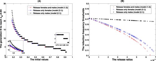
We end the whole manuscript with numerical trials for answering the second question, i.e. how supplemental releases of infected mosquitoes lower the infection frequency threshold to make the persistence achievable. To this end, still letting $s_f=0.1$, $s_h=0.9$, $\mu =0.05$, we plot the infection frequency thresholds for the release ratios lying in $(0,0.007)$ in Figure 7(B). Here we take 0.007 to guarantee the existence of the thresholds under three release strategies. And numerical observation agree with our theoretical results that higher release ratios lead to lower infection frequency thresholds to guarantee the success of Wolbachia persistence.

Disclosure statement

No potential conflict of interest was reported by the author(s).

Additional information

Funding

This work was supported by National Natural Science Foundation of China [grant numbers 12071095,11971127, 11631005], Program for Changjiang Scholars and Innovative Research Team in University [grant number IRT_16R16] and Innovative Research Grant for the Postgraduates of Guangzhou University [grant number 2020GDJC-D10].

References

- C. Ahlbrandt and A.C. Peterson, Discrete Hamiltonian System, Springer, Boston, MA, 2010.
- H.N. Aida, H. Dieng, A.T. Nurita, M.C. Salmah, F. Miake, and B. Norasmah, The biology and demographic parameters of Aedes albopictus in northern peninsular Malaysia, Asian Pac. J. Trop. Biomed. 1(6) (2011), pp. 472–477.
- F. Arkin, Dengue researcher faces charges in vaccine fiasco, Science 364 (2019), pp. 320.
- F. Baldacchino, B. Caputo, F. Chandre, A. Drago, A. Della Torre, F. Montarsi, and A. Rizzolli, Control methods against invasive Aedes mosquitoes in Europe: A review, Pest Manag. Sci. 71(11) (2015), pp. 1471–1485.
- G. Bian, D. Joshi, Y. Dong, P. Lu, G. Zhou, X. Pan, Y. Xu, G. Dimopoulos, and Z. Xi, Wolbachia invades Anopheles stephensi populations and induces refractoriness to plasmodium infection, Science340 (2013), pp. 748–751.
- E. Caspari and G.S. Watson, On the evolutionary importance of cytoplasmic sterility in mosquitoes, Evolution 13(4) (1959), pp. 568–570.
- J. Cohen, Dengue may bring out the worst in Zika, Science 356(6332) (2017), pp. 175–180.
- W. Dejnirattisai, P. Supasa, W. Wongwiwat, A. Rouvinski, G. Barba-Spaeth, T. Duangchinda, A.Sakuntabhai, V.M. Cao-Lormeau, P. Malasit, and F.A. Rey, Dengue virus sero-cross-reativity drives antibody-dependent enhancement of infection with Zika virus, Nat. Immunol. 17 (2016), pp. 1102–1109.
- S. Elaydi, An Introduction to Difference Equations, Springer, New York, 2005.
- P.E.M. Fine, On the dynamics of symbiote-dependent cytoplasmic incompatibility in Culicine mosquitoes, J. Invertebr. Pathol. 31(1) (1978), pp. 10–18.
- J. Guarnera and G.L. Hale, Four human diseases with significant public health impact caused by mosquito-borne flaviviruses: West Nile, Zika, dengue and yellow fever, Semin. Diagn. Pathol. 36(3) (2019), pp. 170–176.
- M. Hertig and S.B. Wolbach, Studies on Rickettsia-like micro-organisms in insects, J. Med. Res. 44(3) (1924), pp. 329–374.
- A.A. Hoffmann, B.L. Montgomery, J. Popovici, I. Iturbe-Ormaetxe, P. Johnson, F. Muzzi, M. Greenfield, M. Durkan, Y.S. Leong, Y. Dong, H. Cook, J. Axford, A.G. Callahan, N. Kenny, C. Omodei, E.A. McGraw, P.A. Ryan, S.A. Ritchie, M. Turelli, and S.L. O'Neill, Successful establishment of Wolbachia in Aedes populations to suppress dengue transmission, Nature 476(7361) (2011), pp. 454–457.
- A.A. Hoffmann, M. Turelli, and L.G. Harshman, Factors affecting the distribution of cytoplasmic incompatibility in Drosophila simulans, Genetics 126(4) (1990), pp. 933–948.
- L. Hu, M. Huang, M. Tang, J. Yu, and B. Zheng, Wolbachia spread dynamics in stochastic environments, Theor. Popul. Biol. 106 (2015), pp. 32–44.
- L. Hu, M. Tang, Z. Wu, Z. Xi, and J. Yu, The threshold infection level for Wolbachia invasion in radom environment, J. Differ. Equ. 266 (2019), pp. 4377–4393.
- M. Huang, L. Hu, and J. Yu, Wolbachia infection dynamics by reaction-diffusion equations, Sci. China Math. 58(1) (2015), pp. 77–96.
- M. Huang, L. Hu, and B. Zheng, Comparing the efficiency of Wolbachia driven Aedes mosquito suppression strategies, J. Appl. Anal. Comput. 9(1) (2019), pp. 211–230.
- M. Huang, J. Luo, L. Hu, B. Zheng, and J. Yu, Assessing the efficiency of Wolbachia driven Aedes mosquito suppression by delay differential equations, J. Theor. Biol. 440(7) (2018), pp. 1–11.
- M. Huang, M. Tang, J. Yu, and B. Zheng, The impact of mating competitiveness and incomplete cytoplasmic incompatibility on Wolbachia-driven mosquito population suppression, Math. Biosci. Eng.16(5) (2019), pp. 4741–4757.
- M. Huang, M. Tang, J. Yu, and B. Zheng, A stage structured model of delay differential equations for Aedes mosquito population suppression, Discrete Contin. Dyn. Syst. 40(6) (2020), pp. 3467–3484.
- Y. Hui, G. Lin, J. Yu, and J. Li, A delayed differential equation model for mosquito population suppression with sterile mosquitoes, Discrete Contin. Dyn. Syst. Ser. B 25(12) (2020), pp. 4659–4676.
- H. Laven, Cytoplasmic inheritance in Culex, Nature 177 (1956), pp. 141–142.
- C.J. Mcmeniman, R.V. Lane, B.N. Cass, A. Fong, M. Sidhu, Y. Wang, and S. O'Neill, Stable introduction of a life-shortening Wolbachia infection into the mosquito Aedes aegypi, Science 323(5910) (2009), pp. 141–144.
- Y. Shi and J. Yu, Wolbachia infection enhancing and decaying domains in mosquito population based on discrete models, J. Biol. Dyn. 14(1) (2020), pp. 679–695.
- P. Somwang, J. Yanola, W. Suwan, C. Walton, N. Lumjuan, L. Prapanthadara, and P. Somboon, Enzymes-based resistant mechanism in pyrethroid resistant and susceptible Aedes aegypti strains from northern Thailand, Parasitol. Res. 109(3) (2011), pp. 531–537.
- M. Turelli, Evolution of incompatibility-inducing microbes and their hosts, Evolution 48(5) (1994), pp. 1500–1513.
- M. Turelli, Cytoplasmic incompatibility in populations with overlapping generations, Evolution 64(1) (2010), pp. 232–241.
- M. Turelli and A.A. Hoffmann, Rapid spread of an inherited incompatibility factor in California Drosophila, Nature 353(6343) (1991), pp. 440–442.
- M. Turelli and A.A. Hoffmann, Cytoplasmic incompatibility in Drosophila simulans: Dynamics and parameter estimates from natural populations, Genetics 140(4) (1995), pp. 1319–1338.
- Y. Wang, X. Liu, C. Li, T. Su, J. Jin, Y. Guo, D. Ren, Z. Yang, Q. Liu, and F. Meng, A survey of insecticide resistance in Aedes albopictus (Diptera: Culicidae) during a 2014 dengue fever outbreak in Guangzhou, China, J. Econ. Entomol. 110(1) (2017), pp. 239–244.
- Z. Xi and S.L. Dobson, Characterization of Wolbachia transfection efficiency by using microinjection of embryonic cytoplasm and embryo homogenate, Appl. Environ. Microbiol. 71(6) (2005), pp. 3199–3204.
- J. Yu, Modelling mosquito population suppression based on delay differential equations, SIAM J. Appl. Math. 78(6) (2018), pp. 3168–3187.
- J. Yu, Existence and stability of a unique and exact two periodic orbits for an interactive wild and sterile mosquito model, J. Differ. Equ. 269(12) (2020), pp. 10395–10415.
- J. Yu and J. Li, Dynamics of interactive wild and sterile mosquitoes with time delay, J. Biol. Dyn.13(4) (2019), pp. 1–15.
- J. Yu and J. Li, Global asymptotic stability in an interactive wild and sterile mosquito model, J. Differ. Equ. 269(7) (2020), pp. 6193–6215.
- J. Yu and B. Zheng, Modeling Wolbachia infection in mosquito population via discrete dynamical models, J. Differ. Equ. Appl. 25(11) (2019), pp. 1549–1567.
- B. Zheng, W. Guo, L. Hu, M. Huang, and J. Yu, Complex Wolbachia infection dynamics in mosquitoes with imperfect maternal transmission, Math. Biosci. Eng. 15(2) (2018), pp. 523–541.
- B. Zheng, M. Tang, and J. Yu, Modeling Wolbachia spread in mosquitoes through delay differential equations , SIAM J. Appl. Math. 74(3) (2014), pp. 743–770.
- B. Zheng, X. Liu, M. Tang, Z. Xi, and J. Yu, Use of age-stage structural models to seek optimal Wolbachia-infected male mosquito releases for mosquito-borne disease control, J. Theor. Biol. 472(7) (2019), pp. 95–109.
- B. Zheng, M. Tang, and J. Yu, Modeling Wolbachia spread in mosquitoes through delay differential equations, SIAM J. Appl. Math. 74(3) (2014), pp. 743–770.
- B. Zheng, M. Tang, J. Yu, and J. Qiu, Wolbachia spreading dynamics in mosquitoes with imperfect maternal transmission, J. Math. Biol. 76(1–2) (2018), pp. 235–263.
- B. Zheng and J. Yu, Existence and uniqueness of periodic orbits in a discrete model on Wolbachia infection frequency, Adv. Nonlinear Anal. 11 (2022), pp. 212–224.
- B. Zheng, J. Yu, and J. Li, Modeling and analysis of the implementation of the Wolbachia incompatible and sterile insect technique for mosquito population suppression, SIAM J. Appl. Math. 81(2) (2021), pp. 718–740.
- B. Zheng, J. Yu, Z. Xi, and M. Tang, The annual abundance of dengue and Zika vector Aedes albopictus and its stubbornness to suppression, Ecol. Model. 387(10) (2018), pp. 38–48.
- X. Zheng, D. Zhang, Y. Li, C. Yang, Y. Wu, X. Liang, Y. Liang, X. Pan, L. Hu, Q. Sun, X. Wang, Y. Wei, J. Zhu, W. Qian, Z. Yan, A. Parker, J. Giles, K. Bourtzis, J. Bouyer, M. Tang, B. Zheng, J. Yu, J. Liu, J. Zhuang, Z. Hu, M. Zhang, J. Gong, X. Hong, Z. Zhang, L. Lin, Q. Liu, Z. Hu, Z. Wu, L. Baton, A. Hoffmann, and Z. Xi, Incompatible and sterile insect techniques combined eliminate mosquitoes, Nature 572(7767) (2019), pp. 56–61.