Full article: A delay non-autonomous model for the combined effects of fear, prey refuge and additional food for predator

Formulae display: $MathJax Logo$ ?Mathematical formulae have been encoded as MathML and are displayed in this HTML version using MathJax in order to improve their display. Uncheck the box to turn MathJax off. This feature requires Javascript. Click on a formula to zoom.

Abstract

In this paper, we investigate the combined effects of fear, prey refuge and additional food for predator in a predator–prey system with Beddington type functional response. We observe oscillatory behaviour of the system in the absence of fear, refuge and additional food whereas the system shows stable dynamics if anyone of these three factors is introduced. After analysing the behaviour of system with fear, refuge and additional food, we find that the system destabilizes due to fear factor whereas refuge and additional food stabilize the system by killing persistent oscillations. We extend our model by considering the fact that after sensing the chemical/vocal cue, prey takes some time for assessing the predation risk. The delayed system shows chaotic dynamics through multiple stability switches for increasing values of time delay. Moreover, we see the impact of seasonal change in the level of fear on the delayed as well as non-delayed system.

Keywords:

1. Introduction

Rapid change in climatic conditions, human activities, upwelling resource pulses etc., have caused extinction of many species around the globe. To maintain the ecological balance and biodiversity, there is an urgent need of conservation of these species. In these situations, only statistical data is not enough to maintain the ecological balance. Indeed, mathematical models can help to better understand the behaviour of ecosystem. The most important factor in a predator–prey model is to observe the type of interactions between prey and predator, affecting dynamical behaviour of the system. There are two types of interaction − one prey dependent which is a function of prey only and the other one is predator dependent which depends on both species. The most widely used functional response in describing predator–prey interactions is the Holling type II functional response, in which per capita predation rate is an increasing, smooth, and saturating function of prey density. However, the prey-dependent functional responses fail to model the interference among predators and have been facing challenges from the biological as well as physiological communities. Some biologists have argued that in many situations, especially when predators have to search for food, the functional response in a predator–prey model should be predator dependent. There are much significant evidences which suggest that predator dependence in the functional response occurs quite frequently in laboratory and natural systems. In order to mediate theoretical and experimental perspectives, Beddington [Citation8] and DeAngelis et al. [Citation21] considered a functional form of prey consumption rate that depends on both the species. They proposed the form, $g = p x / (a x + b y + c)$ , which is similar to the Holling type II functional response with the extra term by in the denominator, which interprets the mutual interference among predators. This functional form is known as Beddington-DeAngelis functional response.

It is well documented that Beddington-DeAngelis type functional response is more acceptable than other available response functions [Citation14, Citation64], and it has the ability to take care of a number of ecological mechanisms. Several mathematical models including the Beddington-DeAngelis type functional response have been investigated [Citation22, Citation26, Citation43], and the results showed that this type of functional form produces very rich and biologically reasonable dynamics. Cantrell and Cosner [Citation14] have studied a predator–prey model with Beddington–DeAngelis functional response, and analysed various dynamical properties like stability, limit cycle, etc. Dimitrov and Kojouharov [Citation22] found that mutual interference between predators can alone stabilize predator–prey interactions. Growing biological and physiological evidences suggest that predator-dependent functional response is more appropriate when predators have a highly competitive food searching process in nature due to limited resources [Citation6, Citation24]. In view of these facts, in the present article, we consider Beddington–DeAngelis functional response as the interaction term between prey and predator.

Over the last few decades researchers paid attention on direct predation only in a predator–prey model as it is easy to observe in real world [Citation1–3, Citation68]. But, recent studies have shown that indirect impact of predator greatly affect the population dynamics [Citation36, Citation37, Citation52, Citation54, Citation61, Citation65, Citation66]. Fear effect plays a pivotal role among the indirect effects. In any habitat, prey feel predation pressure as a result they exhibit anti-predator behaviour like foraging, habitat change, different physiological change, etc. Scared species forage less. Due to fear of predator, prey acquires different mechanisms like reduction in mating, starvation, migration from vulnerable place to invulnerable which actually lessen their growth rate. For example, scared Mule deer opt for lesser foraging to avoid the acute predation risk of mountain lions [Citation5]. Creel et al. [Citation17] observed that elks alter their reproductive physiology due to the fear of wolves. Such complex strategies play a central role in the evolutionary processes. Candolin [Citation13] observed that threespine stickleback males regulate their reproductive decisions by assessing the threat of predation. The empirical evidences by Zanette et al. [Citation74] established that offspring generation of song sparrow is demographically impressed and reduced by 40% due to the perceived threat of predation. In their experiment, they actively prevented the chances of direct killing with the help of electric fencing and seine netting, and imitated the predation risk by broadcasting predator call playbacks over an entire breeding season of song sparrows. Modelling the impact of fear effect on the dynamic interaction of prey and predator has gained commendable attentions among researchers after the seminal work of Wang et al. [Citation69]. Panday et al. [Citation53] investigated a three species food chain model by considering that the growth rates of prey and middle predator are reduced due to fear of middle and top predators, respectively. In [Citation40], authors discussed the control of chaotic dynamics in a three species food chain model with fear. Zhang et al. [Citation75] showed that the fear effect not only reduces the predator population but also stabilizes the system by excluding periodic solutions.

If predator can not reach to a portion of prey, it means prey species are able to take refuge. Refuge is an anti-predator behaviour which can help to prolong a predator–prey interaction by reducing the chance of extinction due to over predation. When prey experience attack cue from predator, they take refuge by changing their functioning like their body colour, shape, size, habitat, etc. Most of the adult preys are capable to take refuge. The first demonstration of this effect was given by Gause in his experiments with the protozoan, Didinium (predator) and Paramecium (prey) [Citation28]. Mite predator–prey interactions often exhibit spatial refugia which afford the prey some degree of protection from predation and reduce the chance of extinction due to predation. In 1970, Connell [Citation16] found that adults of the barnacle, Balanus glandula, were safe from predatory snails of the genus, Thais, in intertidal areas which are submerged only for a short period of time during high tide. The mature barnacles were restricted to refuge in the areas where Thais was present but not where Thais was absent, suggesting that the refuge prevents Thais from eliminating Balanus. Dolbeer and Clark [Citation23] found that snowshoe hare (prey) prefers forested habitat with dense undercover, where they are relatively safe from their predator (e.g. Canada lynx). Additional food is any kind of food or species other than focal/basal prey. Additional food to the predator acquire less attention than focal prey. Due to fear and refuge, prey availability reduces to a great extent to the predator and as a consequence predator population goes to extinction. To maintain ecological balance or to sustain predator population in the system, additional foods are provided to predator. Joint effects of reduction in prey refuge and the presence of appropriate amount of additional food can control the prey population [Citation7, Citation15, Citation20, Citation30, Citation59, Citation62]. Das and Samanta [Citation19] studied the effects of fear and additional food for predator in a fluctuating environment. The findings of Wang et al. [Citation67] showed that for a certain level of fear, prey refuge is beneficial for the coexistence of prey and predator populations. Recently, Mondal and Samanta [Citation51] studied the dynamics of a delayed predator–prey system with nonlinear prey refuge under the influence of fear effect and additional food for predator. Note that in these studies, authors have considered that a constant proportion of prey population is taking refuge, but, in a realistic scenario, refuge depends on predator density [Citation49, Citation63].

It is well understood that time delay occurs often in almost every biological situation. Several studies have been done with retarded systems which explored different dynamics of the systems including periodic oscillation, persistence, bifurcation and chaos of populations [Citation9, Citation10, Citation18, Citation29, Citation46]. The process of perceiving predator signals through chemical and/or vocal cues and the changes in life history and behavioural responses in the prey population conceals some time delay. Panday et al. [Citation55] investigated the impact of such time delay in a two dimensional predator–prey system. They observed that for the gradual increase in the magnitude of delay, the system dynamics switches multiple times between stable focus and limit cycle oscillations, and ultimately enters into the chaotic regime. Mondal et al. [Citation50] investigated the impact of gestation delay in a predator–prey system with fear effect and additional food for predator. Kumar and Dubey [Citation39] studied the fear effect and prey refuge in a predator–prey system with gestation delay; they observed that the system enters into chaotic regime for larger values of gestation delay.

Seasonality can be defined as the regular and periodic changes of variable on an annual time scale [Citation70]. Seasonal variables relevant in ecological systems not only include temperature, photoperiod but also include rainfall, wind, human activity, etc. [Citation45, Citation60]. The recognition of these varied drivers of ecological systems shows the ubiquity of seasonality. When the environmental fluctuation is taken into account, a model must be non-autonomous. The level of fear may vary due to change in predation pressure, intraspecific competition or resource distribution among the individuals [Citation25, Citation32]. A predator–prey model with seasonal variation of fear effect is studied by Roy and Alam [Citation58]. Sk et al. [Citation62] investigated the joint effects of fear, refuge and additional food on the dynamic interactions of prey and predator by allowing the respective parameter to vary seasonally; complex dynamics such as higher periodic solutions and bursting patterns were observed due to variations in the seasonally forced parameters.

In the present investigation, our first goal is to explore the combined effects of fear of predator, prey refuge and additional food for predator with modified Beddington type functional response. The fraction of prey population taking refuge is assumed to depend on the predator density. Our another goal is to investigate the effect of time delay involved in the process of perceiving predator signals and behavioural responses by the prey population. Finally, we see the impact of seasonal variation of fear of predator in the systems with and without time delay.

2. The mathematical model

To construct the model, we consider water bugs as prey and fish as predator [Citation44]. In the presence of fish, the bugs become scarce, and measurable densities (a proportion of water bugs depending on predator density) are restricted to areas with thick aquatic vegetation. As a result, scarce prey which are spending time in refuges also typically costs prey in terms of reduced feeding, mating opportunities, competition, etc. So, for fish, available water bugs reduced in a great amount. Due to less prey (water bugs), predators (fish) interfere with one another. Therefore, fish need additional food to persist in the system. We can also consider snowshoe hare (prey) and Canada lynx (predator) as another example of species for our proposed model. Let at any time t>0, N (number per unit area) be the density of prey population and P (number per unit area) be the density of predator population in the region under consideration. In the modelling process, the following assumptions are made.

Prey population grows with $r_{0}$ as its intrinsic growth rate and $r_{1}$ as mortality rate due to intraspecific competition when there is no predation and fear effect. The reason behind considering the intraspecific competition among the species of prey population is that for high density of prey population and less availability of resources, the individuals of prey population compete with each other for the available resources.
The effect of fear not only influence the reproduction of prey but also has the potential to affect the death rate of the prey population [Citation42, Citation72, Citation73]. Thus, the growth rate of prey population should be multiplied by a factor that decreases with the increase in level of fear and the density of predator population. In view of this, the growth rate ( $r_{0}$ ) is multiplied by a factor $\frac{1}{1 + k P}$ , which accounts for the cost of anti-predator behaviour of prey due to fear of predation [Citation62, Citation69]. Here, the constant k measures the level of fear.
The prey population has capability to take refuge, which provides them a degree of protection against predation. However, the refuge behaviour of prey population is affected by the number of predator population present in the area. So, the proportion of prey population taking refuge is considered to be a function of predator population [Citation49, Citation63].
The interactions between prey and predator populations are assumed to be governed by modified Beddington type functional response [Citation15].
The predator population is supposed to be supplied with an additional food of biomass A, which is assumed to be distributed uniformly in their habitat. The additional food is assumed to be non-reproducing and is supplied at a constant rate. The number of encounters per predator with additional food is proportional to the density of additional food. Moreover, providing additional food to predator population reduces the rate at which predators consume the prey items.
The density of predator population decreases in the region due to natural death at a constant rate d.

Keeping these assumptions in mind, our proposed model is represented by the following system of differential equations: (1) $\begin{aligned} \frac{d N}{d t} & = \frac{r_{0} N}{1 + k P} - r_{1} N^{2} - \frac{α (1 - m P) N P}{θ + ξ η A + b (1 - m P) N + c P}, \\ \frac{d P}{d t} & = \frac{β {α (1 - m P) N + η A} P}{θ + ξ η A + b (1 - m P) N + c P} - d P . \end{aligned}$ (1)

Throughout this paper, we consider the acceptable range $0 \leq (1 - m P) \leq 1$ , i.e. $P \leq \frac{1}{m}$ . Parameters involved in system (Equation1(1) $\begin{aligned} \frac{d N}{d t} & = \frac{r_{0} N}{1 + k P} - r_{1} N^{2} - \frac{α (1 - m P) N P}{θ + ξ η A + b (1 - m P) N + c P}, \\ \frac{d P}{d t} & = \frac{β {α (1 - m P) N + η A} P}{θ + ξ η A + b (1 - m P) N + c P} - d P . \end{aligned}$ (1) ) are assumed to be constant and have positive values. The initial conditions are given by (2) $N (0) = N_{0} > 0, P (0) = P_{0} > 0.$ (2) In Table , we have mentioned the biological meanings of the parameters involved in system (Equation1(1) $\begin{aligned} \frac{d N}{d t} & = \frac{r_{0} N}{1 + k P} - r_{1} N^{2} - \frac{α (1 - m P) N P}{θ + ξ η A + b (1 - m P) N + c P}, \\ \frac{d P}{d t} & = \frac{β {α (1 - m P) N + η A} P}{θ + ξ η A + b (1 - m P) N + c P} - d P . \end{aligned}$ (1) ).

Table 1. Biological meanings of parameters involved in system (Equation1(1) $\begin{aligned} \frac{d N}{d t} & = \frac{r_{0} N}{1 + k P} - r_{1} N^{2} - \frac{α (1 - m P) N P}{θ + ξ η A + b (1 - m P) N + c P}, \\ \frac{d P}{d t} & = \frac{β {α (1 - m P) N + η A} P}{θ + ξ η A + b (1 - m P) N + c P} - d P . \end{aligned}$ (1) ) and their values used for numerical simulations.

Display Table

3. Mathematical analysis of system (1)

3.1. Positivity and boundedness of system's solutions

Positivity: The positivity of state variables (system's solutions) of system (Equation1(1) $\begin{aligned} \frac{d N}{d t} & = \frac{r_{0} N}{1 + k P} - r_{1} N^{2} - \frac{α (1 - m P) N P}{θ + ξ η A + b (1 - m P) N + c P}, \\ \frac{d P}{d t} & = \frac{β {α (1 - m P) N + η A} P}{θ + ξ η A + b (1 - m P) N + c P} - d P . \end{aligned}$ (1) ) implies that the population never go to extinction and always survive in the system.

To prove the positivity of the solutions of system (Equation1(1) $\begin{aligned} \frac{d N}{d t} & = \frac{r_{0} N}{1 + k P} - r_{1} N^{2} - \frac{α (1 - m P) N P}{θ + ξ η A + b (1 - m P) N + c P}, \\ \frac{d P}{d t} & = \frac{β {α (1 - m P) N + η A} P}{θ + ξ η A + b (1 - m P) N + c P} - d P . \end{aligned}$ (1) ), we integrate both equations of system (Equation1(1) $\begin{aligned} \frac{d N}{d t} & = \frac{r_{0} N}{1 + k P} - r_{1} N^{2} - \frac{α (1 - m P) N P}{θ + ξ η A + b (1 - m P) N + c P}, \\ \frac{d P}{d t} & = \frac{β {α (1 - m P) N + η A} P}{θ + ξ η A + b (1 - m P) N + c P} - d P . \end{aligned}$ (1) ) over the limit 0 to t, and get $\begin{aligned} N (t) & = N (0) \exp \{\int_{0}^{t} [\frac{r_{0}}{1 + k P (s)} - r_{1} N (s) \\ - \frac{α (1 - m P (s)) P (s)}{θ + ξ η A + b (1 - m P (s)) N (s) + c P (s)}] d s\}, \\ P (t) & = P (0) \exp \{\int_{0}^{t} [\frac{β {α (1 - m P (s)) N (s) + η A}}{θ + ξ η A + b (1 - m P (s)) N (s) + c P (s)} - d] d s\} . \end{aligned}$ Since $N (0), P (0) > 0$ , we have $N (t), P (t) > 0$ for all $t \geq 0$ . Therefore, any solution initiating in the positive quadrant of $R^{2}$ always remains therein. Hence, the interior of the first quadrant of $R^{2}$ is an invariant set.

Boundedness: In theoretical ecology, boundedness of a system implies that the system is well behaved. Boundedness of the solutions entails that none of the interacting populations grow exponentially for a long-time interval.

Theorem 3.1

All the solutions of the system (Equation1(1) $\begin{aligned} \frac{d N}{d t} & = \frac{r_{0} N}{1 + k P} - r_{1} N^{2} - \frac{α (1 - m P) N P}{θ + ξ η A + b (1 - m P) N + c P}, \\ \frac{d P}{d t} & = \frac{β {α (1 - m P) N + η A} P}{θ + ξ η A + b (1 - m P) N + c P} - d P . \end{aligned}$ (1) ) are uniformly bounded.

Proof.

We note from the first equation of system (Equation1(1) $\begin{aligned} \frac{d N}{d t} & = \frac{r_{0} N}{1 + k P} - r_{1} N^{2} - \frac{α (1 - m P) N P}{θ + ξ η A + b (1 - m P) N + c P}, \\ \frac{d P}{d t} & = \frac{β {α (1 - m P) N + η A} P}{θ + ξ η A + b (1 - m P) N + c P} - d P . \end{aligned}$ (1) ) that $\frac{d N}{d t} \leq r_{0} N - r_{1} N^{2} = N (r_{0} - r_{1} N) .$ Therefore, $\underset{t \to \infty}{lim sup} N (t) \leq \frac{r_{0}}{r_{1}}$ .

Thus, for an arbitrary small $ϵ_{1} > 0$ , there exists $T_{1} > 0$ such that for some $M_{1}$ $N (t) \leq \frac{r_{0}}{r_{1}} + ϵ_{1} = M_{1} \forall t > T_{1} .$ Again, from the second equation of the system (Equation1(1) $\begin{aligned} \frac{d N}{d t} & = \frac{r_{0} N}{1 + k P} - r_{1} N^{2} - \frac{α (1 - m P) N P}{θ + ξ η A + b (1 - m P) N + c P}, \\ \frac{d P}{d t} & = \frac{β {α (1 - m P) N + η A} P}{θ + ξ η A + b (1 - m P) N + c P} - d P . \end{aligned}$ (1) ), for all $t > T_{1}$ , we have $\frac{d P}{d t} \leq \frac{β (α M_{1} + η A) P}{c P} - d P = \frac{β (α M_{1} + η A)}{c} - d P .$ Applying the theory of differential inequality [Citation41], we obtain $0 < P (t) < \frac{β (α M_{1} + η A)}{c d} + \{P (0) - \frac{β (α M_{1} + η A)}{c d}\} e^{- d t} .$ Hence, as $t \to \infty$ , for m>0, we have $0 \leq P (t) \leq \frac{β (α M_{1} + η A)}{c d} = \frac{1}{m}$ , where $m = \frac{c d}{β (α M_{1} + η A)}$ .

Therefore, solutions of the system (Equation1(1) $\begin{aligned} \frac{d N}{d t} & = \frac{r_{0} N}{1 + k P} - r_{1} N^{2} - \frac{α (1 - m P) N P}{θ + ξ η A + b (1 - m P) N + c P}, \\ \frac{d P}{d t} & = \frac{β {α (1 - m P) N + η A} P}{θ + ξ η A + b (1 - m P) N + c P} - d P . \end{aligned}$ (1) ) are bounded above. Thus, the region of attraction for all solutions of system (Equation1(1) $\begin{aligned} \frac{d N}{d t} & = \frac{r_{0} N}{1 + k P} - r_{1} N^{2} - \frac{α (1 - m P) N P}{θ + ξ η A + b (1 - m P) N + c P}, \\ \frac{d P}{d t} & = \frac{β {α (1 - m P) N + η A} P}{θ + ξ η A + b (1 - m P) N + c P} - d P . \end{aligned}$ (1) ) initiating in the positive quadrant is given by the following set: $Ω = \{(N, P) : 0 \leq N (t) \leq M_{1}, 0 \leq P (t) \leq \frac{1}{m}\},$ which is closed and bounded in the positive cone of the two dimensional plane.

3.2. System's equilibria

Due to nonlinearity of model system (Equation1(1) $\begin{aligned} \frac{d N}{d t} & = \frac{r_{0} N}{1 + k P} - r_{1} N^{2} - \frac{α (1 - m P) N P}{θ + ξ η A + b (1 - m P) N + c P}, \\ \frac{d P}{d t} & = \frac{β {α (1 - m P) N + η A} P}{θ + ξ η A + b (1 - m P) N + c P} - d P . \end{aligned}$ (1) ), it is not possible to find exact solutions to the system. Instead, we determine the long-term behaviour of the system. In general, a nonlinear system either gravitates towards an equilibrium point or it blows up. An equilibrium point represents the rest state of a dynamical system. These points can be obtained by putting the growth rate of different variables of model system (Equation1(1) $\begin{aligned} \frac{d N}{d t} & = \frac{r_{0} N}{1 + k P} - r_{1} N^{2} - \frac{α (1 - m P) N P}{θ + ξ η A + b (1 - m P) N + c P}, \\ \frac{d P}{d t} & = \frac{β {α (1 - m P) N + η A} P}{θ + ξ η A + b (1 - m P) N + c P} - d P . \end{aligned}$ (1) ) equal to zero.

The equilibria of system (Equation1(1) $\begin{aligned} \frac{d N}{d t} & = \frac{r_{0} N}{1 + k P} - r_{1} N^{2} - \frac{α (1 - m P) N P}{θ + ξ η A + b (1 - m P) N + c P}, \\ \frac{d P}{d t} & = \frac{β {α (1 - m P) N + η A} P}{θ + ξ η A + b (1 - m P) N + c P} - d P . \end{aligned}$ (1) ) are obtained as follows.

The population-free equilibrium $E_{0} = (0, 0)$ , which always exists.
The predator-free equilibrium $E_{1} = (N_{1}, 0)$ , where $N_{1} = r_{0} r_{1}^{- 1}$ . The equilibrium $E_{1}$ always exists.
The prey-free equilibrium $E_{2} = (0, P_{2})$ , where $P_{2} = \frac{η A (β - d ξ) - d θ}{c d}$ . The equilibrium $E_{2}$ exists if (3) $A > \frac{d θ}{η (β - d ξ)} .$ (3)
The coexistence equilibrium $E^{*} = (N^{*}, P^{*})$ , where $N^{*} = \frac{η A (d ξ - β) + d (θ + c P^{*})}{(1 - m P^{*}) (β α - b d)}$ and $P^{*}$ is the positive solution(s) of the following biquadratic equation: (4) $A_{4} P^{4} + A_{3} P^{3} + A_{2} P^{2} + A_{1} P + A_{0} = 0,$ (4) where $\begin{aligned} A_{4} = k m^{2} α (β α - b d)^{2}, A_{3} = m α (m - 2 k) (β α - b d)^{2} + c^{2} d r_{1} k β α, \\ A_{2} = α (β α - b d) {c m r_{0} β + (k - 2 m) (β α - b d)} + c d r_{1} (c β α + k S_{2}) + c k β α S_{1}, \\ A_{1} = α (β α - b d)^{2} + S_{2} (c d r_{1} + k S_{1}) + c β α S_{1} - r_{0} (β α - b d) (c β α - m S_{2}), \\ A_{0} = S_{2} {S_{1} - r_{0} (β α - b d)} \end{aligned}$ with $S_{1} = r_{1} {d θ + η A (d ξ - β)}$ and $S_{2} = β {α θ + η A (α ξ - b)}$ . Clearly, $A_{4}$ is positive. Thus, Equation (Equation4(4) $A_{4} P^{4} + A_{3} P^{3} + A_{2} P^{2} + A_{1} P + A_{0} = 0,$ (4) ) has at least one positive root if $A_{0}$ is negative.

Remark 3.1

In the equilibrium $E_{0}$ , where there is no species in the system, it should not be possible to observe it in the real ecosystem. That is, this equilibrium point should be unstable. In the equilibrium $E_{1}$ , where there is no predator population in the system, it should be possible to observe it in some special circumstances. That is, this equilibrium can be stable under certain conditions. The equilibrium $E_{2}$ represents the case when ecosystem is free from prey population and only predators survive. This is possible because the predators depend upon additional food apart from their focal prey. For the existence of this equilibrium, the amount of additional food must be in accordance with the ability to detect and handle additional food, conversion efficiency, and death rate of predator. Finally, the equilibrium $E^{*}$ , where both prey and predator are present, is very common in natural ecosystem. Thus, it should be stable in some ecosystems. It is worthy to note that the stability of coexistence equilibrium will be helpful for the biological conservation programs.

3.3. Stability analysis

In this section, we perform the local stability analysis of the equilibria of system (Equation1(1) $\begin{aligned} \frac{d N}{d t} & = \frac{r_{0} N}{1 + k P} - r_{1} N^{2} - \frac{α (1 - m P) N P}{θ + ξ η A + b (1 - m P) N + c P}, \\ \frac{d P}{d t} & = \frac{β {α (1 - m P) N + η A} P}{θ + ξ η A + b (1 - m P) N + c P} - d P . \end{aligned}$ (1) ). The local stability analysis characterizes whether or not the system settles to the equilibrium point if its state is initiated close to, but not precisely at a given equilibrium point. The equilibrium point is said to be locally asymptotically stable if there is a neighbourhood of the equilibrium point such that for all initial starts in that neighbourhood, the system approaches to the equilibrium point as $t \to \infty$ [Citation57]. The local stability of all equilibria of system (Equation1(1) $\begin{aligned} \frac{d N}{d t} & = \frac{r_{0} N}{1 + k P} - r_{1} N^{2} - \frac{α (1 - m P) N P}{θ + ξ η A + b (1 - m P) N + c P}, \\ \frac{d P}{d t} & = \frac{β {α (1 - m P) N + η A} P}{θ + ξ η A + b (1 - m P) N + c P} - d P . \end{aligned}$ (1) ) is stated in the following theorem.

Theorem 3.2

(1)	The equilibrium $E_{0}$ is always unstable.
(2)	The equilibrium $E_{1}$ is stable if the following condition holds: (5) $\frac{β (α r_{0} + r_{1} η A)}{b r_{0} + r_{1} (θ + ξ η A)} - d < 0.$ (5)
(3)	The equilibrium $E_{2}$ , if exists, is stable if the following conditions hold: (6) $\frac{r_{0}}{1 + k P_{2}} - \frac{α P_{2} (1 - m P_{2})}{θ + ξ η A + c P_{2}} < 0, \frac{β η A (θ + ξ η A)}{(θ + ξ η A + c P_{2})^{2}} - d < 0.$ (6)
(4)	The equilibrium $E^{*}$ , if exists, is locally asymptotically stable if and only if $B_{1} > 0$ and $B_{2} > 0$ , where $B_{1}$ and $B_{2}$ are defined in the proof.

Proof.

Stability of the equilibria $E_{0}$ , $E_{1}$ and $E_{2}$ can be shown by evaluating the Jacobian of system (Equation1(1) $\begin{aligned} \frac{d N}{d t} & = \frac{r_{0} N}{1 + k P} - r_{1} N^{2} - \frac{α (1 - m P) N P}{θ + ξ η A + b (1 - m P) N + c P}, \\ \frac{d P}{d t} & = \frac{β {α (1 - m P) N + η A} P}{θ + ξ η A + b (1 - m P) N + c P} - d P . \end{aligned}$ (1) ) at these equilibria and determining signs of the real parts of the eigenvalues. At the equilibrium $E^{*}$ , the Jacobian of system (Equation1(1) $\begin{aligned} \frac{d N}{d t} & = \frac{r_{0} N}{1 + k P} - r_{1} N^{2} - \frac{α (1 - m P) N P}{θ + ξ η A + b (1 - m P) N + c P}, \\ \frac{d P}{d t} & = \frac{β {α (1 - m P) N + η A} P}{θ + ξ η A + b (1 - m P) N + c P} - d P . \end{aligned}$ (1) ) reduces to $J_{E^{*}} = [a_{i j}]$ , where $\begin{aligned} a_{11} & = \frac{r_{0}}{1 + k P^{*}} - 2 r_{1} N^{*} - \frac{α P^{*} (1 - m P^{*}) (θ ξ η A + c P^{*})}{{θ + ξ η A + b (1 - m P^{*}) N^{*} + c P^{*}}^{2}}, \\ a_{12} & = - \frac{k r_{0} N^{*}}{(1 + k P^{*})^{2}} - \frac{α N^{*} (1 - 2 m P^{*})}{θ + ξ η A + b (1 - m P^{*}) N^{*} + c P^{*}} \\ + \frac{α (1 - m P^{*}) N^{*} P^{*} (c - b m N^{*})}{{θ + ξ η A + b (1 - m P^{*}) N^{*} + c P^{*}}^{2}}, \\ a_{21} & = \frac{β (1 - m P^{*}) P^{*} {η A (α ξ - b) + α (θ + c P^{*})}}{{θ + ξ η A + b (1 - m P^{*}) N^{*} + c P^{*}}^{2}}, \\ a_{22} & = \frac{β {α (1 - m P^{*}) N^{*} + η A - α m N^{*} P^{*}}}{θ + ξ η A + b (1 - m P^{*}) N^{*} + c P^{*}} \\ - \frac{β P^{*} (c - b m N^{*}) {α (1 - m P^{*}) N^{*} + η A}}{{θ + ξ η A + b (1 - m P^{*}) N^{*} + c P^{*}}^{2}} - d . \end{aligned}$ The corresponding characteristic equation is obtained as (7) $λ^{2} + B_{1} λ + B_{2} = 0,$ (7) where $B_{1} = - (a_{11} + a_{22})$ and $B_{2} = a_{11} a_{22} - a_{12} a_{21}$ . By Routh-Hurwitz criterion, we claim that roots of Equation (Equation7(7) $λ^{2} + B_{1} λ + B_{2} = 0,$ (7) ) are either negative or have negative real parts if and only if $B_{1}, B_{2} > 0$ .

Remark 3.2

The first point of above theorem indicates that it is not possible to observe the equilibrium without prey and predator. The second point of this theorem shows that the predator-free ecosystem is achieved only if the growth rate of predator due to consumption of prey and additional food is lower than its natural death. It is apparent from the third point of the above theorem that for stability of prey-free equilibrium, the fear of predator and the growth rate of predator due to additional food should be high, predator consume more prey, growth rate of prey is less due to fear and also prey take less refuge. The last point of Theorem 3.2 tells that if the initial state of system (Equation1(1) $\begin{aligned} \frac{d N}{d t} & = \frac{r_{0} N}{1 + k P} - r_{1} N^{2} - \frac{α (1 - m P) N P}{θ + ξ η A + b (1 - m P) N + c P}, \\ \frac{d P}{d t} & = \frac{β {α (1 - m P) N + η A} P}{θ + ξ η A + b (1 - m P) N + c P} - d P . \end{aligned}$ (1) ) is near the equilibrium point $E^{*}$ , then the solution trajectories not only stay near the equilibrium $E^{*}$ for all t>0, but also approach to the components of equilibrium $E^{*}$ as $t \to \infty$ . Thus, if the initial values of state variables N and P are close to $N^{*}$ and $P^{*}$ , respectively, then the system (Equation1(1) $\begin{aligned} \frac{d N}{d t} & = \frac{r_{0} N}{1 + k P} - r_{1} N^{2} - \frac{α (1 - m P) N P}{θ + ξ η A + b (1 - m P) N + c P}, \\ \frac{d P}{d t} & = \frac{β {α (1 - m P) N + η A} P}{θ + ξ η A + b (1 - m P) N + c P} - d P . \end{aligned}$ (1) ) will eventually get stabilized provided $B_{1} > 0$ and $B_{2} > 0$ . That is, small perturbations in system's variables do not affect stability of the system at the coexistence equilibrium point.

3.4. Hopf-bifurcation analysis

Now, we consider m as a bifurcation parameter and investigate the occurrence of Hopf-bifurcation through the coexistence equilibrium point $E^{*}$ , keeping the remaining parameters fixed. Hopf bifurcation with respect to m means that there exists a critical value of m at which systems's stability switches and a periodic solution arises from stable state. Existence of Hopf bifurcation ensures survivability of all species in oscillatory mode, which actually fit with our ecological subsystem. In this context, we have the following theorem.

Theorem 3.3

If there exists a critical value of m (say $m = m^{*}$ ) such that $B_{1} (m^{*}) = 0$ , $B_{2} (m^{*}) > 0$ and $[\frac{d R e (λ (m))}{d m}]_{m = m^{*}} \neq 0.$ Then, the system (Equation1(1) $\begin{aligned} \frac{d N}{d t} & = \frac{r_{0} N}{1 + k P} - r_{1} N^{2} - \frac{α (1 - m P) N P}{θ + ξ η A + b (1 - m P) N + c P}, \\ \frac{d P}{d t} & = \frac{β {α (1 - m P) N + η A} P}{θ + ξ η A + b (1 - m P) N + c P} - d P . \end{aligned}$ (1) ) undergoes Hopf-bifurcation through the equilibrium $E^{*}$ at $m = m^{*}$ .

Proof.

To determine the nature of equilibrium $E^{*}$ , we require the sign of the real parts of the roots of the characteristic Equation (Equation7(7) $λ^{2} + B_{1} λ + B_{2} = 0,$ (7) ). Let $λ (m) = u (m) + i v (m)$ be one of the eigenvalues of the characteristic Equation (Equation7(7) $λ^{2} + B_{1} λ + B_{2} = 0,$ (7) ). Substituting the value of $λ$ in Equation (Equation7(7) $λ^{2} + B_{1} λ + B_{2} = 0,$ (7) ), and separating real and imaginary parts, we get (8) $\begin{aligned} u^{2} - v^{2} + B_{1} u + B_{2} = 0, \end{aligned}$ (8) (9) $\begin{aligned} 2 u v + B_{1} v = 0. \end{aligned}$ (9) A necessary condition for the change of stability through the equilibrium $E^{*}$ is that the characteristic Equation (Equation7(7) $λ^{2} + B_{1} λ + B_{2} = 0,$ (7) ) should have purely imaginary roots. We set $m = m^{*}$ such that $u (m^{*}) = 0$ , and put u = 0 in Equations (Equation8(8) $\begin{aligned} u^{2} - v^{2} + B_{1} u + B_{2} = 0, \end{aligned}$ (8) ) and (Equation9(9) $\begin{aligned} 2 u v + B_{1} v = 0. \end{aligned}$ (9) ). Then, we have (10) $\begin{aligned} - v^{2} + B_{2} = 0, \end{aligned}$ (10) (11) $\begin{aligned} B_{1} v = 0, v \neq 0. \end{aligned}$ (11) From Equations (Equation10(10) $\begin{aligned} - v^{2} + B_{2} = 0, \end{aligned}$ (10) ) and (Equation11(11) $\begin{aligned} B_{1} v = 0, v \neq 0. \end{aligned}$ (11) ), we have $B_{1} (m^{*}) = 0$ and $v (m^{*}) = \sqrt{B_{2} (m^{*})}$ , which implies $λ (m^{*}) = i \sqrt{B_{2} (m^{*})}$ .

The eigenvalues of the characteristic Equation (Equation7(7) $λ^{2} + B_{1} λ + B_{2} = 0,$ (7) ) are $λ_{1, 2} = \frac{- B_{1} \pm \sqrt{B_{1}^{2} - 4 B_{2}}}{2} .$ Here, $B_{1}$ and $B_{2}$ are the functions of the parameter m, when other parameter values are fixed. Moreover, we assume there exists some $m = m^{*}$ such that $B_{1} (m^{*}) = 0$ and $B_{2} (m^{*}) > 0$ . Therefore, the positive real parts of these eigenvalues change the sign when m passes through $m^{*}$ . Consequently, the system switches its stability provided that the transversality condition is satisfied.

Differentiating Equations (Equation8(8) $\begin{aligned} u^{2} - v^{2} + B_{1} u + B_{2} = 0, \end{aligned}$ (8) ) and (Equation9(9) $\begin{aligned} 2 u v + B_{1} v = 0. \end{aligned}$ (9) ) with respect to m, and put u = 0, we have $B_{1} \frac{d u}{d m} - 2 v \frac{d v}{d m} = - \frac{d B_{2}}{d m}, 2 v \frac{d u}{d m} + B_{1} \frac{d v}{d m} = - v \frac{d B_{1}}{d m} .$ From the above equations, we get ${[\frac{d R e (λ (m))}{d m}]}_{m = m^{*}} = {[\frac{2 v^{2} \frac{d B_{1}}{d m} + B_{1} \frac{d B_{2}}{d m}}{B_{1}^{2} + 4 v^{2}}]}_{m = m^{*}},$ which is non-zero if ${[2 v^{2} \frac{d B_{1}}{d m} + B_{1} \frac{d B_{2}}{d m}]}_{m = m^{*}} \neq 0.$

4. Effect of time lag involved in the fear of predation

In this section, we modify our previous model system (Equation1(1) $\begin{aligned} \frac{d N}{d t} & = \frac{r_{0} N}{1 + k P} - r_{1} N^{2} - \frac{α (1 - m P) N P}{θ + ξ η A + b (1 - m P) N + c P}, \\ \frac{d P}{d t} & = \frac{β {α (1 - m P) N + η A} P}{θ + ξ η A + b (1 - m P) N + c P} - d P . \end{aligned}$ (1) ) by incorporating a discrete time delay. After sensing the chemical or vocal cue, prey takes some times for assessing the predation risk. Therefore, the prey does not respond instantaneously to the population size of the predator species, rather there must be some time lag [Citation11, Citation55]. In order to incorporate this time lag, we consider that at time t, the fear of predator is in accordance with the predator density at time $t - τ$ (for some $τ > 0$ ). Incorporating this time lag in system (Equation1(1) $\begin{aligned} \frac{d N}{d t} & = \frac{r_{0} N}{1 + k P} - r_{1} N^{2} - \frac{α (1 - m P) N P}{θ + ξ η A + b (1 - m P) N + c P}, \\ \frac{d P}{d t} & = \frac{β {α (1 - m P) N + η A} P}{θ + ξ η A + b (1 - m P) N + c P} - d P . \end{aligned}$ (1) ), we get the following system of delay differential equations: (12) $\begin{aligned} \frac{d N}{d t} & = \frac{r_{0} N}{1 + k P (t - τ)} - r_{1} N^{2} - \frac{α (1 - m P) N P}{θ + ξ η A + b (1 - m P) N + c P}, \\ \frac{d P}{d t} & = \frac{β {α (1 - m P) N + η A} P}{θ + ξ η A + b (1 - m P) N + c P} - d P . \end{aligned}$ (12) The initial conditions for the system (Equation12(12) $\begin{aligned} \frac{d N}{d t} & = \frac{r_{0} N}{1 + k P (t - τ)} - r_{1} N^{2} - \frac{α (1 - m P) N P}{θ + ξ η A + b (1 - m P) N + c P}, \\ \frac{d P}{d t} & = \frac{β {α (1 - m P) N + η A} P}{θ + ξ η A + b (1 - m P) N + c P} - d P . \end{aligned}$ (12) ) take the form (13) $N (ζ) = κ_{1} (ζ), P (ζ) = κ_{2} (ζ), - τ \leq ζ \leq 0,$ (13) where $κ = (κ_{1}, κ_{2})^{T} \in C$ such that $κ_{i} (ζ) \geq 0, i = 1, 2 \forall ζ \in [- τ, 0]$ and $C_{+}$ denotes the Banach space $C_{+} ([- τ, 0], R_{+ 0}^{2})$ of continuous functions mapping the interval $[- τ, 0]$ into $R_{+ 0}^{2}$ and denotes the norm of an element $κ \in C_{+}$ by $∥ κ ∥ = sup_{- τ \leq ζ \leq 0} {| κ_{1} (ζ) |, | κ_{2} (ζ) |}$ . For biological feasibility, we further assume that $κ_{i} (0) \geq 0$ for i = 1, 2.

4.1. Stability analysis in the presence of time delay

Now, we study the stability behaviour of the system (Equation12(12) $\begin{aligned} \frac{d N}{d t} & = \frac{r_{0} N}{1 + k P (t - τ)} - r_{1} N^{2} - \frac{α (1 - m P) N P}{θ + ξ η A + b (1 - m P) N + c P}, \\ \frac{d P}{d t} & = \frac{β {α (1 - m P) N + η A} P}{θ + ξ η A + b (1 - m P) N + c P} - d P . \end{aligned}$ (12) ) in the presence of time delay around the coexistence equilibrium $E^{*}$ . Linearizing the system (Equation12(12) $\begin{aligned} \frac{d N}{d t} & = \frac{r_{0} N}{1 + k P (t - τ)} - r_{1} N^{2} - \frac{α (1 - m P) N P}{θ + ξ η A + b (1 - m P) N + c P}, \\ \frac{d P}{d t} & = \frac{β {α (1 - m P) N + η A} P}{θ + ξ η A + b (1 - m P) N + c P} - d P . \end{aligned}$ (12) ) about the coexistence equilibrium point $E^{*} = (N^{*}, P^{*})$ , we get (14) $\frac{d X}{d t} = R X (t) + S X (t - τ),$ (14) where $R = (\begin{array}{cc} r_{11} & r_{12} \\ r_{21} & r_{22} \end{array}), S = (\begin{array}{cc} 0 & s_{12} \\ 0 & 0 \end{array}), X (\cdot) = (\begin{array}{cc} n (\cdot) \\ p (\cdot) \end{array})$ with $\begin{aligned} r_{11} = \frac{r_{0}}{1 + k P^{*}} - 2 r_{1} N^{*} - \frac{α P^{*} (1 - m P^{*}) (θ + ξ η A + c P^{*})}{{θ + ξ η A + b (1 - m P^{*}) N^{*} + c P^{*}}^{2}}, \\ r_{12} = - \frac{α N^{*} (1 - 2 m P^{*})}{θ + ξ η A + b (1 - m P^{*}) N^{*} + c P^{*}} + \frac{α (1 - m P^{*}) N^{*} P^{*} (c - b m N^{*})}{{θ + ξ η A + b (1 - m P^{*}) N^{*} + c P^{*}}^{2}}, \\ r_{21} = \frac{β (1 - m P^{*}) P^{*} {η A (α ξ - b) + α (θ + c P^{*})}}{{θ + ξ η A + b (1 - m P^{*}) N^{*} + c P^{*}}^{2}}, \\ r_{22} = - \frac{β α m N^{*} P^{*}}{θ + ξ η A + b (1 - m P^{*}) N^{*} + c P^{*}} - \frac{β P^{*} (c - b m N^{*}) {α (1 - m P^{*}) N^{*} + η A}}{{θ + ξ η A + b (1 - m P^{*}) N^{*} + c P^{*}}^{2}}, \\ s_{12} = - \frac{k r_{0} N^{*}}{(1 + k P^{*})^{2}} . \end{aligned}$ Here, n and p are small perturbations around the equilibrium point $(N^{*}, P^{*})$ .

The characteristic equation for the linearized system (Equation14(14) $\frac{d X}{d t} = R X (t) + S X (t - τ),$ (14) ) corresponding to equilibrium $E^{*}$ is given by (15) $λ^{2} + b_{1} λ + b_{0} + c_{0} e^{- λ τ} = 0,$ (15) where $b_{1} = - (r_{11} + r_{22}), b_{0} = r_{11} r_{22} - r_{12} r_{21}, c_{0} = r_{21} s_{12} .$ For $τ = 0$ , all the roots of Equation (Equation15(15) $λ^{2} + b_{1} λ + b_{0} + c_{0} e^{- λ τ} = 0,$ (15) ) are either negative or have negative real parts provided $b_{1} > 0$ and $b_{0} + c_{0} > 0$ while for $τ > 0$ , it has infinitely many roots. By Rouche's Theorem and continuity in τ, stability of Equation (Equation15(15) $λ^{2} + b_{1} λ + b_{0} + c_{0} e^{- λ τ} = 0,$ (15) ) will change if the real part of the leading roots crosses imaginary axis, i.e. if Equation (Equation15(15) $λ^{2} + b_{1} λ + b_{0} + c_{0} e^{- λ τ} = 0,$ (15) ) has purely imaginary roots. Hence, putting $λ = i ω$ $(ω > 0)$ in Equation (Equation15(15) $λ^{2} + b_{1} λ + b_{0} + c_{0} e^{- λ τ} = 0,$ (15) ), and separating real and imaginary parts, we get (16) $\begin{aligned} c_{0} \sin (ω τ) & = b_{1} ω, \end{aligned}$ (16) (17) $\begin{aligned} - c_{0} \cos (ω τ) & = b_{0} - ω^{2} . \end{aligned}$ (17) Squaring and adding Equations (Equation16(16) $\begin{aligned} c_{0} \sin (ω τ) & = b_{1} ω, \end{aligned}$ (16) ) and (Equation17(17) $\begin{aligned} - c_{0} \cos (ω τ) & = b_{0} - ω^{2} . \end{aligned}$ (17) ), we get (18) $c_{0}^{2} = (b_{0} - ω^{2})^{2} + b_{1}^{2} ω^{2} .$ (18) Substituting $ω^{2} = ψ$ in Equation (Equation18(18) $c_{0}^{2} = (b_{0} - ω^{2})^{2} + b_{1}^{2} ω^{2} .$ (18) ), we obtain the following equation: (19) $Ψ (ψ) \equiv ψ^{2} + a_{1} ψ + a_{0} = 0,$ (19) where $a_{1} = b_{1}^{2} - 2 b_{0}$ and $a_{0} = b_{0}^{2} - c_{0}^{2}$ .

Note that Equation (Equation19(19) $Ψ (ψ) \equiv ψ^{2} + a_{1} ψ + a_{0} = 0,$ (19) ) has exactly one positive root if $a_{0}$ is negative, and two positive roots if $a_{0}$ is positive and $a_{1}$ is negative.

Theorem 4.1

Suppose that the equilibrium $E^{*}$ exists and is locally asymptotically stable for $τ = 0$ . Also, let $ψ_{0} = ω_{0}^{2}$ be a positive root of Equation (Equation19(19) $Ψ (ψ) \equiv ψ^{2} + a_{1} ψ + a_{0} = 0,$ (19) ). Then, there exists $τ^{*} = min_{n \geq 0} τ_{n}^{*}$ such that the equilibrium $E^{*}$ of the system (Equation12(12) $\begin{aligned} \frac{d N}{d t} & = \frac{r_{0} N}{1 + k P (t - τ)} - r_{1} N^{2} - \frac{α (1 - m P) N P}{θ + ξ η A + b (1 - m P) N + c P}, \\ \frac{d P}{d t} & = \frac{β {α (1 - m P) N + η A} P}{θ + ξ η A + b (1 - m P) N + c P} - d P . \end{aligned}$ (12) ) is asymptotically stable for $0 \leq τ \leq τ^{*}$ and unstable for $τ > τ^{*}$ , where $τ_{n}^{*} = \frac{1}{ω_{0}} \tan^{- 1} [\frac{b_{1} ω_{0}}{ω_{0}^{2} - b_{0}}] + \frac{n π}{ω_{0}},$ for $n = 0, 1, 2, 3, \dots$ . Moreover, the system (Equation12(12) $\begin{aligned} \frac{d N}{d t} & = \frac{r_{0} N}{1 + k P (t - τ)} - r_{1} N^{2} - \frac{α (1 - m P) N P}{θ + ξ η A + b (1 - m P) N + c P}, \\ \frac{d P}{d t} & = \frac{β {α (1 - m P) N + η A} P}{θ + ξ η A + b (1 - m P) N + c P} - d P . \end{aligned}$ (12) ) undergoes a Hopf-bifurcation at the equilibrium $E^{*}$ when $τ = τ^{*}$ provided $Ψ^{'} (ω_{0}^{2}) > 0$ .

Proof.

Since $ψ = ω_{0}^{2}$ is a solution of Equation (Equation19(19) $Ψ (ψ) \equiv ψ^{2} + a_{1} ψ + a_{0} = 0,$ (19) ), the characteristic Equation (Equation15(15) $λ^{2} + b_{1} λ + b_{0} + c_{0} e^{- λ τ} = 0,$ (15) ) has a pair of purely imaginary roots $\pm i ω_{0}$ . It follows from Equations (Equation16(16) $\begin{aligned} c_{0} \sin (ω τ) & = b_{1} ω, \end{aligned}$ (16) ) and (Equation17(17) $\begin{aligned} - c_{0} \cos (ω τ) & = b_{0} - ω^{2} . \end{aligned}$ (17) ) that $τ_{n}^{*}$ is a function of $ω_{0}$ for $n = 0, 1, 2, 3, \dots$ . Thus, if the system (Equation12(12) $\begin{aligned} \frac{d N}{d t} & = \frac{r_{0} N}{1 + k P (t - τ)} - r_{1} N^{2} - \frac{α (1 - m P) N P}{θ + ξ η A + b (1 - m P) N + c P}, \\ \frac{d P}{d t} & = \frac{β {α (1 - m P) N + η A} P}{θ + ξ η A + b (1 - m P) N + c P} - d P . \end{aligned}$ (12) ) is locally asymptotically stable around the coexistence equilibrium $E^{*}$ for $τ = 0$ , then by Butler's lemma, the equilibrium $E^{*}$ will remain stable for $τ < τ^{*}$ and unstable for $τ > τ^{*}$ such that $τ^{*} = min_{n \geq 0} τ_{n}^{*}$ provided the following transversality condition holds: $s g n {[\frac{d (R e (λ))}{d τ}]}_{τ = τ^{*}} \neq 0.$ Differentiating Equation (Equation15(15) $λ^{2} + b_{1} λ + b_{0} + c_{0} e^{- λ τ} = 0,$ (15) ) with respect to τ, we get $\frac{d λ}{d τ} = \frac{c_{0} λ e^{- λ τ}}{2 λ + b_{1} - c_{0} τ e^{- λ τ}} \Rightarrow {(\frac{d λ}{d τ})}^{- 1} = \frac{2 λ + b_{1}}{c_{0} λ e^{- λ τ}} - \frac{τ}{λ} .$ Now, $\begin{aligned} s g n {[\frac{d (R e (λ))}{d τ}]}_{τ = τ^{*}} & = s g n {[\frac{d (R e (λ))}{d τ}]}_{τ = τ^{*}}^{- 1} = s g n {[R e {(\frac{d λ}{d τ})}^{- 1}]}_{λ = i ω_{0}} \\ = s g n [\frac{2 ω_{0}^{2} + a_{1}}{c_{0}^{2}}] = s g n [\frac{Ψ^{'} (ω_{0}^{2})}{c_{0}^{2}}] . \end{aligned}$ Clearly, $Ψ^{'} (ω_{0}^{2}) \neq 0$ , since $ω_{0}^{2}$ is a simple positive root of Equation (Equation19(19) $Ψ (ψ) \equiv ψ^{2} + a_{1} ψ + a_{0} = 0,$ (19) ). Therefore, the transversality condition is verified and hence Hopf-bifurcation occurs at $τ = τ^{*}$ , i.e. a family of periodic solutions bifurcate from the equilibrium $E^{*}$ as τ passes through $τ^{*}$ [Citation31].

Remark 4.1

If Equation (Equation19(19) $Ψ (ψ) \equiv ψ^{2} + a_{1} ψ + a_{0} = 0,$ (19) ) has two positive real roots $ψ_{+}$ (corresponds to $ω_{+}^{2}$ ) and $ψ_{-}$ (corresponds to $ω_{-}^{2}$ ), where $ψ_{+} > ψ_{-}$ , i.e. the characteristic Equation (Equation15(15) $λ^{2} + b_{1} λ + b_{0} + c_{0} e^{- λ τ} = 0,$ (15) ) has two pair of purely imaginary roots $\pm i ω_{\pm}$ , then we have (20) $τ_{n}^{*} = \frac{1}{ω_{\pm}} \tan^{- 1} [\frac{b_{1} ω_{\pm}}{ω_{\pm}^{2} - b_{0}}] + \frac{n π}{ω_{\pm}}$ (20) for $n = 0, 1, 2, 3, \dots$ . If the following transversality conditions are satisfied, ${s g n [\frac{d (R e (λ))}{d τ}]}_{τ = τ_{+}^{*}} > 0, {s g n [\frac{d (R e (λ))}{d τ}]}_{τ = τ_{-}^{*}} < 0,$ then there exists a positive integer q such that there are q switches from stability to instability and back to stability. In other words, when $τ \in [0, τ_{0 +}^{*}), (τ_{0 -}^{*}, τ_{1_{+}}^{*}), \dots, (τ_{(q - 1)_{-}}^{*}, τ_{q_{+}}^{*})$ , the equilibrium $E^{*}$ is stable, and when $τ \in (τ_{0 +}^{*}, τ_{0 -}^{*}), (τ_{1_{+}}^{*}, τ_{1_{-}}^{*})$ , $\dots, (τ_{(q - 1)_{+}}^{*}, τ_{(q - 1)_{-}}^{*})$ , the equilibrium $E^{*}$ is unstable. Therefore, Hopf-bifurcations occur around the equilibrium $E^{*}$ at $τ_{n_{\pm}}^{*}$ for $n = 0, 1, 2, 3, \dots$ .

5. Direction and stability of Hopf-bifurcation

Previously, we have shown that the system (Equation12(12) $\begin{aligned} \frac{d N}{d t} & = \frac{r_{0} N}{1 + k P (t - τ)} - r_{1} N^{2} - \frac{α (1 - m P) N P}{θ + ξ η A + b (1 - m P) N + c P}, \\ \frac{d P}{d t} & = \frac{β {α (1 - m P) N + η A} P}{θ + ξ η A + b (1 - m P) N + c P} - d P . \end{aligned}$ (12) ) undergoes Hopf-bifurcation at the coexistence equilibrium $E^{*} = (N^{*}, P^{*})$ when τ passes through $τ^{*}$ . In this section, we investigate the direction and stability of Hopf-bifurcating solutions at $τ = τ^{*}$ for system (Equation12(12) $\begin{aligned} \frac{d N}{d t} & = \frac{r_{0} N}{1 + k P (t - τ)} - r_{1} N^{2} - \frac{α (1 - m P) N P}{θ + ξ η A + b (1 - m P) N + c P}, \\ \frac{d P}{d t} & = \frac{β {α (1 - m P) N + η A} P}{θ + ξ η A + b (1 - m P) N + c P} - d P . \end{aligned}$ (12) ) by using the techniques of normal form theory and centre manifold theorem [Citation34]. We calculate the values of $μ_{2}$ , $β_{2}$ and $τ_{2}$ , which determine the direction of Hopf-bifurcation, stability of bifurcating periodic solutions and period of bifurcating periodic solutions, respectively. In this regard, we state the following theorem.

Theorem 5.1

(1)	The Hopf-bifurcation is supercritical or subcritical if $μ_{2} > 0$ or $μ_{2} < 0$ , and the bifurcating periodic solutions exist for $τ > τ^{}$ or $τ < τ^{}$ .
(2)	The bifurcating periodic solutions are stable or unstable according as $β_{2} < 0$ or $β_{2} > 0$ .
(3)	The period of the bifurcating periodic solutions increases or decreases according as $τ_{2} > 0$ or $τ_{2} < 0$ .

Proof.

Let us consider the transformations $X_{1} (t) = N - N^{*}$ , $X_{2} (t) = P - P^{*}$ and $τ = τ^{*} + ν$ , $ν \in R$ . Then, $ν = 0$ is the Hopf-bifurcation value of system (Equation12(12) $\begin{aligned} \frac{d N}{d t} & = \frac{r_{0} N}{1 + k P (t - τ)} - r_{1} N^{2} - \frac{α (1 - m P) N P}{θ + ξ η A + b (1 - m P) N + c P}, \\ \frac{d P}{d t} & = \frac{β {α (1 - m P) N + η A} P}{θ + ξ η A + b (1 - m P) N + c P} - d P . \end{aligned}$ (12) ). Now, system (Equation12(12) $\begin{aligned} \frac{d N}{d t} & = \frac{r_{0} N}{1 + k P (t - τ)} - r_{1} N^{2} - \frac{α (1 - m P) N P}{θ + ξ η A + b (1 - m P) N + c P}, \\ \frac{d P}{d t} & = \frac{β {α (1 - m P) N + η A} P}{θ + ξ η A + b (1 - m P) N + c P} - d P . \end{aligned}$ (12) ) can be written in the form (21) $\dot{X} (t) = L_{ν} (X_{t}) + F (ν, X_{t}),$ (21) where $X (t) = (X_{1} (t), X_{2} (t))^{T} \in R^{2}$ . For $κ = (κ_{1}, κ_{2})^{T} \in C ([- 1, 0], R_{+}^{2})$ , $L_{ν} : C \to R$ and $F : R \times C \to R$ are given by (22) $\begin{aligned} L_{ν} (κ) & = (τ^{*} + ν) B^{0} (\begin{matrix} κ_{1} (0) \\ κ_{2} (0) \end{matrix}) + (τ^{*} + ν) B^{1} (\begin{matrix} κ_{1} (- 1) \\ κ_{2} (- 1) \end{matrix}), \end{aligned}$ (22) (23) $\begin{aligned} F (ν, κ) & = (τ^{*} + ν) B^{2}, \end{aligned}$ (23) with $\begin{aligned} B^{0} = (\begin{array}{cc} r_{11} & r_{12} \\ r_{21} & r_{22} \end{array}), B^{1} = (\begin{array}{cc} 0 & s_{12} \\ 0 & 0 \end{array}), \\ B^{2} = (\begin{matrix} s_{1} κ_{1}^{2} (0) + s_{2} κ_{1} (0) κ_{2} (0) + s_{3} κ_{2}^{2} (0) + s_{4} κ_{1} (0) κ_{2} (- 1) \\ s_{5} κ_{1}^{2} (0) + s_{6} κ_{1} (0) κ_{2} (0) + s_{7} κ_{2}^{2} (0) \end{matrix}), \end{aligned}$ where $r_{i j}$ (i, j = 1, 2) and $s_{12}$ are defined earlier, and $\begin{aligned} s_{1} & = - 2 r_{1} + \frac{2 b α P^{*} (1 - m P^{*})^{2} (θ + ξ η A + c P^{*})}{{θ + ξ η A + b (1 - m P^{*}) N^{*} + c P^{*}}^{3}}, \\ s_{2} & = - \frac{k r_{0}}{(1 + k P^{*})^{2}} - \frac{α (1 - 2 m P^{*}) (θ + ξ η A + c P^{*})}{{θ + ξ η A + b (1 - m P^{*}) N^{*} + c P^{*}}^{2}} \\ + \frac{2 α P^{*} (1 - m P^{*}) (θ + ξ η A + c P^{*}) (c - b m N^{*})}{{θ + ξ η A + b (1 - m P^{*}) N^{*} + c P^{*}}^{3}}, \\ s_{3} & = \frac{2 r_{0} k^{2} N^{*}}{(1 + k P^{*})^{3}} + \frac{2 α N^{*} (c - b m N^{*}) (1 - 2 m P^{*})}{{θ + ξ η A + b (1 - m P^{*}) N^{*} + c P^{*}}^{2}} \\ + \frac{2 m α N^{*} {θ + ξ η A + b (1 - m P^{*}) N^{*} + c P^{*}}^{2} - 2 α N^{*} P^{*} (1 - m P^{*}) (c - b m N^{*})^{2}}{{θ + ξ η A + b (1 - m P^{*}) N^{*} + c P^{*}}^{3}}, \\ s_{4} & = - \frac{k r_{0}}{(1 + k P^{*})^{2}}, s_{5} = - \frac{2 b β P^{*} (1 - m P^{*})^{2} {η A (α ξ - b) + α (θ + c P^{*})}}{{θ + ξ η A + b (1 - m P^{*}) N^{*} + c P^{*}}^{3}}, \\ s_{6} & = \frac{β [(1 - 2 m P^{*}) {η A (α ξ - b) + α (θ + c P^{*})} + c α P^{*} (1 - m P^{*})]}{{θ + ξ η A + b (1 - m P^{*}) N^{*} + c P^{*}}^{2}} \\ - \frac{2 β P^{*} (1 - m P^{*}) (c - b m N^{*}) {η A (α ξ - b) + α (θ + c P^{*})}}{{θ + ξ η A + b (1 - m P^{*}) N^{*} + c P^{*}}^{3}}, \\ s_{7} & = - \frac{β (c - b m N^{*}) {α N^{*} (1 - 2 m P^{*}) + η A}}{{θ + ξ η A + b (1 - m P^{*}) N^{*} + c P^{*}}^{2}} \\ + \frac{\begin{matrix} 2 β P^{*} (c - b m N^{*})^{2} {α (1 - m P^{*}) N^{*} + η A} \\ - 2 α β m N^{*} {θ + ξ η A + b (1 - m P^{*}) N^{*} + c P^{*}}^{2} \end{matrix}}{{θ + ξ η A + b (1 - m P^{*}) N^{*} + c P^{*}}^{3}} . \end{aligned}$ By the Riesz representation theorem, there exists a function $γ (σ, ν)$ of bounded variation for $σ \in [- 1, 0]$ such that (24) $L_{ν} κ = \int_{- 1}^{0} d γ (σ, ν) κ (σ), f o r κ \in C .$ (24) In fact, $γ (σ, ν) = (τ^{*} + ν) (\begin{array}{cc} r_{11} & r_{12} \\ r_{21} & r_{22} \end{array}) δ (σ) - (τ^{*} + ν) (\begin{array}{cc} 0 & s_{12} \\ 0 & 0 \end{array}) δ (σ + 1),$ where δ is the Dirac delta function.

For $κ \in C^{1} ([- 1, 0], R_{+}^{2})$ , define $D (ν) κ = \{\begin{array}{cc} \frac{d κ (σ)}{d σ}, & σ \in [- 1, 0), \\ \int_{- 1}^{0} d γ (ν, s) κ (s), & σ = 0 \end{array}$ and $R (ν) κ = \{\begin{array}{cc} 0, & σ \in [- 1, 0), \\ F (ν, κ), & σ = 0. \end{array}$ The system (Equation21(21) $\dot{X} (t) = L_{ν} (X_{t}) + F (ν, X_{t}),$ (21) ) is of the form (25) $\dot{X} (t) = D (ν) X_{t} + R (ν) X_{t},$ (25) where $X_{t} (σ) = X_{t} (t + σ)$ for $σ \in [- 1, 0]$ .

For $ζ \in C^{1} ([0, 1], (R_{+}^{2})^{*})$ , define $D^{*} ζ (s) = \{\begin{array}{cc} - \frac{d ζ (s)}{d s}, & s \in (0, 1], \\ \int_{- 1}^{0} d γ^{T} (t, 0) ζ (- t), & s = 0 \end{array}$ and a bilinear inner product (26) $〈 ζ (s), κ (σ) 〉 = \bar{ζ} (0) κ (0) - \int_{- 1}^{0} \int_{ρ = 0}^{σ} \bar{ζ} (ρ - σ) d γ (σ) κ (ρ) d ρ,$ (26) where $γ (σ) = γ (σ, 0)$ . Clearly, $D (0)$ and $D^{*}$ are adjoint operators. We know that $\pm i ω_{0} τ^{*}$ are eigenvalues of $D (0)$ . So, they are also eigenvalues of $D^{*}$ . Now, we search for the eigenvector of $D (0)$ and $D^{*}$ corresponding to $i ω_{0} τ^{*}$ and $- i ω_{0} τ^{*}$ , respectively.

Now, we assume that $q (σ) = (1, u)^{T} e^{i ω_{0} τ^{*} σ}$ and $q^{*} (s)$ are the eigenvectors of $D (0)$ and $D^{*}$ for the eigenvalues $i ω_{0} τ^{*}$ and $- i ω_{0} τ^{*}$ , respectively. Then, we have $D (0) q (σ) = i ω_{0} τ^{*} q (σ)$ . Using the definition of $D (0)$ and from (Equation24(24) $L_{ν} κ = \int_{- 1}^{0} d γ (σ, ν) κ (σ), f o r κ \in C .$ (24) ), we have $τ^{*} (\begin{array}{cc} r_{11} - i ω_{0} & r_{12} + s_{12} e^{- i ω_{0} τ^{*}} \\ r_{21} & r_{22} \end{array}) q (0) = (\begin{matrix} 0 \\ 0 \end{matrix}) .$ Hence, $q (0) = (1, u)^{T}$ and $q^{*} (s) = H (1, u^{*})^{T} e^{i ω_{0} τ^{*} s}$ , where (27) $u = \frac{r_{21}}{i ω_{0} - r_{22}}, u^{*} = - \frac{r_{11} + i ω_{0}}{r_{21}} .$ (27) We need to determine the value of H in such a way that $〈 q^{*} (s), q (σ) 〉 = 1$ , $〈 q^{*} (s), \bar{q} (σ) 〉 = 0$ . Therefore, $\begin{aligned} 〈 q^{*} (s), q (σ) 〉 & = \bar{H} (1, \bar{u^{*}}) (1, u)^{T} - \int_{- 1}^{0} \int_{ς = 0}^{σ} \bar{H} (1, \bar{u^{*}}) e^{- i ω_{0} τ^{*} (ς - σ)} d γ (σ) (1, u)^{T} e^{i ω_{0} τ^{*} ς} d ς \\ = \bar{H} [1 + \bar{u^{*}} u - \int_{- 1}^{0} (1, \bar{u^{*}}) σ e^{i ω_{0} τ^{*} σ} d γ (σ) (1, u)^{T}] \\ = \bar{H} [1 + \bar{u^{*}} u + τ^{*} \bar{u^{*}} s_{12} u e^{- i ω_{0} τ^{*}}], \end{aligned}$ which implies $\bar{H} = \frac{1}{1 + \bar{u^{*}} u + τ^{*} \bar{u^{*}} s_{12} u e^{- i ω_{0} τ^{*}}} .$

To describe the centre manifold $C_{0}$ at $ν = 0$ , we compute the coordinates by using the same notations and procedures as proposed by Hassard et al. [Citation34]. Let $X_{t}$ be the solution of Equation (Equation21(21) $\dot{X} (t) = L_{ν} (X_{t}) + F (ν, X_{t}),$ (21) ) at $ν = 0$ . Define (28) $U (t) = 〈 q^{*}, X_{t} 〉, V (t, σ) = x_{t} (σ) - 2 R e {U (t) q (σ)} .$ (28) On the centre manifold $C$ , we have $V (t, σ) = V (U (t), \bar{U} (t), σ)$ , where $V (U (t), \bar{U} (t), σ) = V_{20} (σ) \frac{U^{2}}{2} + V_{11} (σ) U \bar{U} + V_{02} (σ) \frac{{\bar{U}}^{2}}{2} + V_{30} (σ) \frac{U^{3}}{6} + \dots,$ U and $\bar{U}$ are local coordinates for centre manifold $C_{0}$ in the direction of $q^{*}$ and ${\bar{q}}^{*}$ . Here, V is real when $X_{t}$ is real. For solution $X_{t} \in C_{0}$ of Equation (Equation21(21) $\dot{X} (t) = L_{ν} (X_{t}) + F (ν, X_{t}),$ (21) ), since $ν = 0$ , we have $\begin{aligned} \dot{U} (t) & = i ω_{0} τ^{*} U + 〈 {\bar{q}}^{*} (σ), F (0, V (U (t), \bar{U} (t), σ) + 2 R e {U q (σ)}) 〉 \\ = i ω_{0} τ^{*} U + {\bar{q}}^{*} (0) F (0, V (U (t), \bar{U} (t), 0) + 2 R e {U q (0)}) 〉 \\ \equiv i ω_{0} τ^{*} U + {\bar{q}}^{*} (0) F_{0} (U, \bar{U}) . \end{aligned}$ Therefore, $\dot{U} (t) = i ω_{0} τ^{*} U + g (U, \bar{U})$ with (29) $g (U, \bar{U}) = {\bar{q}}^{*} (0) F_{0} (U, \bar{U}) = g_{20} \frac{U^{2}}{2} + g_{11} U \bar{U} + g_{02} \frac{{\bar{U}}^{2}}{2} + g_{21} \frac{U^{2} \bar{U}}{2} + \dots .$ (29) Then, from Equation (Equation28(28) $U (t) = 〈 q^{*}, X_{t} 〉, V (t, σ) = x_{t} (σ) - 2 R e {U (t) q (σ)} .$ (28) ), we obtain (30) $\begin{aligned} X_{t} (σ) & = (X_{1 t} (σ), X_{2 t} (σ)) = V (t, σ) + 2 R e {U (t) q (σ)} \\ = V_{20} (σ) \frac{U^{2}}{2} + V_{11} (σ) U \bar{U} + V_{02} (σ) \frac{{\bar{U}}^{2}}{2} + (1, u)^{T} e^{i ω_{0} τ^{*} σ} U + (1, \bar{u})^{T} e^{- i ω_{0} τ^{*} σ} \bar{U} \\ + O (| (U, \bar{U}) |^{3}) . \end{aligned}$ (30) Thus, from Equation (Equation29(29) $g (U, \bar{U}) = {\bar{q}}^{*} (0) F_{0} (U, \bar{U}) = g_{20} \frac{U^{2}}{2} + g_{11} U \bar{U} + g_{02} \frac{{\bar{U}}^{2}}{2} + g_{21} \frac{U^{2} \bar{U}}{2} + \dots .$ (29) ), we have $\begin{aligned} g (U, \bar{U}) & = {\bar{q}}^{*} (0) F_{0} (U, \bar{U}) \\ = \bar{H} (1, \bar{u^{*}}) τ^{*} (\begin{matrix} s_{1} X_{1 t}^{2} (0) + s_{2} X_{1 t} (0) X_{2 t} (0) + s_{3} X_{2 t}^{2} (0) + s_{4} X_{1 t} (0) X_{2 t} (- 1) \\ s_{5} X_{1 t}^{2} (0) + s_{6} X_{1 t} (0) X_{2 t} (0) + s_{7} X_{2 t}^{2} (0) \end{matrix}) \\ = \bar{H} τ^{*} [s_{1} {\{U + \bar{U} + V_{20}^{1} (0) \frac{U^{2}}{2} + V_{11}^{1} (0) U \bar{U} + V_{02}^{1} (0) \frac{{\bar{U}}^{2}}{2} + O (| (U, \bar{U}) |^{3})\}}^{2} \\ + s_{2} \{U + \bar{U} + V_{20}^{1} (0) \frac{U^{2}}{2} + V_{11}^{1} (0) U \bar{U} + V_{02}^{1} (0) \frac{{\bar{U}}^{2}}{2} + O (| (U, \bar{U}) |^{3})\} \\ \times \{u U + \bar{u} \bar{U} + V_{20}^{2} (0) \frac{U^{2}}{2} + V_{11}^{2} (0) U \bar{U} + V_{02}^{2} (0) \frac{{\bar{U}}^{2}}{2} + O (| (U, \bar{U}) |^{3})\} \\ + s_{3} {\{u U + \bar{u} \bar{U} + V_{20}^{2} (0) \frac{U^{2}}{2} + V_{11}^{2} (0) U \bar{U} + V_{02}^{2} (0) \frac{{\bar{U}}^{2}}{2} + O (| (U, \bar{U}) |^{3})\}}^{2} \\ s_{4} \{U + \bar{U} + V_{20}^{1} (0) \frac{U^{2}}{2} + V_{11}^{1} (0) U \bar{U} + V_{02}^{1} (0) \frac{{\bar{U}}^{2}}{2} + O (| (U, \bar{U}) |^{3})\} \\ \times \{e^{- i ω_{0} τ^{*}} u U + e^{- i ω_{0} τ^{*}} \bar{u} \bar{U} + V_{20}^{2} (- 1) \frac{U^{2}}{2} \\ + V_{11}^{2} (- 1) U \bar{U} + V_{02}^{2} (- 1) \frac{{\bar{U}}^{2}}{2} + O (| (U, \bar{U}) |^{3})\}] \\ \bar{H} τ^{*} \bar{u^{*}} [s_{5} {\{U + \bar{U} + V_{20}^{1} (0) \frac{U^{2}}{2} + V_{11}^{1} (0) U \bar{U} + V_{02}^{1} (0) \frac{{\bar{U}}^{2}}{2} + O (| (U, \bar{U}) |^{3})\}}^{2} \\ + s_{6} \{U + \bar{U} + V_{20}^{1} (0) \frac{U^{2}}{2} + V_{11}^{1} (0) U \bar{U} + V_{02}^{1} (0) \frac{{\bar{U}}^{2}}{2} + O (| (U, \bar{U}) |^{3})\} \\ \times \{u U + \bar{u} \bar{U} + V_{20}^{2} (0) \frac{U^{2}}{2} + V_{11}^{2} (0) U \bar{U} + V_{02}^{2} (0) \frac{{\bar{U}}^{2}}{2} + O (| (U, \bar{U}) |^{3})\} \\ + s_{7} {\{u U + \bar{u} \bar{U} + V_{20}^{2} (0) \frac{U^{2}}{2} + V_{11}^{2} (0) U \bar{U} + V_{02}^{2} (0) \frac{{\bar{U}}^{2}}{2} + O (| (U, \bar{U}) |^{3})\}}^{2}] . \end{aligned}$ Comparing the coefficients of above equations with Equation (Equation29(29) $g (U, \bar{U}) = {\bar{q}}^{*} (0) F_{0} (U, \bar{U}) = g_{20} \frac{U^{2}}{2} + g_{11} U \bar{U} + g_{02} \frac{{\bar{U}}^{2}}{2} + g_{21} \frac{U^{2} \bar{U}}{2} + \dots .$ (29) ), we get (31) $\begin{aligned} g_{20} & = \bar{H} τ^{*} [s_{1} + (s_{2} + s_{6} \bar{u^{*}}) u + (s_{3} + s_{7} \bar{u^{*}}) u^{2} + s_{4} u e^{- i ω_{0} τ^{*}} + s_{5} \bar{u^{*}}], \\ g_{11} & = 2 \bar{H} τ^{*} [s_{1} + (s_{2} + s_{6} \bar{u^{*}}) ℜ u + (s_{3} + s_{7} \bar{u^{*}}) | u |^{2} + s_{4} e^{- i ω_{0} τ^{*}} ℜ u + s_{5} \bar{u^{*}}], \\ g_{02} & = \bar{H} τ^{*} [s_{1} + (s_{2} + s_{6} \bar{u^{*}}) \bar{u} + (s_{3} + s_{7} \bar{u^{*}}) {\bar{u}}^{2} + s_{4} \bar{u} e^{- i ω_{0} τ^{*}} + s_{5} \bar{u^{*}}], \\ g_{21} & = \bar{H} τ^{*} [(s_{1} + s_{5} \bar{u^{*}}) (V_{20}^{1} (0) + 2 V_{11}^{1} (0)) \\ + (s_{2} + s_{6} \bar{u^{*}}) \{V_{11}^{2} (0) + u V_{11}^{1} (0) + \frac{1}{2} (V_{20}^{2} (0) + \bar{u} V_{20}^{1} (0))\} \\ + (s_{3} + s_{7} \bar{u^{*}}) (\bar{u} V_{20}^{2} (0) + 2 u V_{11}^{1} (0)) \\ + s_{4} \{V_{11}^{2} (- 1) + u e^{- i ω_{0} τ^{*}} V_{11}^{1} (0) + \frac{1}{2} (V_{20}^{2} (- 1) + \bar{u} e^{- i ω_{0} τ^{*}} V_{20}^{1} (0))\}] . \end{aligned}$ (31) To calculate the value of $g_{21}$ , we need to compute the values of $V_{20} (σ)$ and $V_{11} (σ)$ . From Equations (Equation25(25) $\dot{X} (t) = D (ν) X_{t} + R (ν) X_{t},$ (25) ) and (Equation28(28) $U (t) = 〈 q^{*}, X_{t} 〉, V (t, σ) = x_{t} (σ) - 2 R e {U (t) q (σ)} .$ (28) ), we have (32) $\begin{aligned} \dot{V} & = {\dot{X}}_{t} - \dot{U} q - \dot{\bar{U}} \bar{q} \\ = \{\begin{array}{cc} D V - 2 R e {{\bar{q}}^{*} (0) F_{0} q (σ)}, & σ \in [- 1, 0) \\ D V - 2 R e {{\bar{q}}^{*} (0) F_{0} q (σ)} + F_{0}, & σ = 0 \end{array} \\ \equiv D V + G (U, \bar{U}, σ), \end{aligned}$ (32) where (33) $G (U, \bar{U}, σ) = G_{20} (σ) \frac{U^{2}}{2} + G_{11} (σ) U \bar{U} + G_{02} (σ) \frac{{\bar{U}}^{2}}{2} + \dots .$ (33) Expanding the above series and comparing the corresponding coefficients, we get (34) $(D - 2 i ω_{0} τ^{*} I) V_{20} (σ) = - G_{20} (σ), D V_{11} (σ) = - G_{11} (σ) .$ (34) From Equation (Equation32(32) $\begin{aligned} \dot{V} & = {\dot{X}}_{t} - \dot{U} q - \dot{\bar{U}} \bar{q} \\ = \{\begin{array}{cc} D V - 2 R e {{\bar{q}}^{*} (0) F_{0} q (σ)}, & σ \in [- 1, 0) \\ D V - 2 R e {{\bar{q}}^{*} (0) F_{0} q (σ)} + F_{0}, & σ = 0 \end{array} \\ \equiv D V + G (U, \bar{U}, σ), \end{aligned}$ (32) ), for $- 1 \leq σ < 0$ , we have (35) $G (U, \bar{U}, σ) = - {\bar{q}}^{*} (0) F_{0} q (σ) - q^{*} (0) {\bar{F}}_{0} \bar{q} (σ) = - g q (σ) - \bar{g} \bar{q} (σ) .$ (35) Comparing the coefficients with Equation (Equation33(33) $G (U, \bar{U}, σ) = G_{20} (σ) \frac{U^{2}}{2} + G_{11} (σ) U \bar{U} + G_{02} (σ) \frac{{\bar{U}}^{2}}{2} + \dots .$ (33) ), we obtain (36) $G_{20} (σ) = - g_{20} q (σ) - {\bar{g}}_{02} \bar{q} (σ), G_{11} (σ) = - g_{11} q (σ) - {\bar{g}}_{11} \bar{q} (σ) .$ (36) Using Equation (Equation34(34) $(D - 2 i ω_{0} τ^{*} I) V_{20} (σ) = - G_{20} (σ), D V_{11} (σ) = - G_{11} (σ) .$ (34) ) and first equation of (Equation36(36) $G_{20} (σ) = - g_{20} q (σ) - {\bar{g}}_{02} \bar{q} (σ), G_{11} (σ) = - g_{11} q (σ) - {\bar{g}}_{11} \bar{q} (σ) .$ (36) ), we have ${\dot{V}}_{20} (σ) = 2 i ω_{0} τ^{*} V_{20} (σ) + g_{20} q (σ) + {\bar{g}}_{02} \bar{q} (σ) .$ Since $q (σ) = (1, u)^{T} e^{i ω_{0} τ^{*} σ}$ , therefore (37) $V_{20} (σ) = \frac{i g_{20}}{ω_{0} τ^{*}} q (0) e^{i ω_{0} τ^{*} σ} + \frac{i {\bar{g}}_{20}}{ω_{0} τ^{*}} \bar{q} (0) e^{- i ω_{0} τ^{*} σ} + E_{1} e^{2 i ω_{0} τ^{*} σ},$ (37) where $E_{1} = (E_{1}^{(1)}, E_{1}^{(2)}) \in R^{2}$ is a constant vector. Similarly, from Equation (Equation34(34) $(D - 2 i ω_{0} τ^{*} I) V_{20} (σ) = - G_{20} (σ), D V_{11} (σ) = - G_{11} (σ) .$ (34) ) and second equation of (Equation36(36) $G_{20} (σ) = - g_{20} q (σ) - {\bar{g}}_{02} \bar{q} (σ), G_{11} (σ) = - g_{11} q (σ) - {\bar{g}}_{11} \bar{q} (σ) .$ (36) ), we obtain (38) $V_{11} (σ) = - \frac{i g_{11}}{ω_{0} τ^{*}} q (0) e^{i ω_{0} τ^{*} σ} + \frac{i {\bar{g}}_{11}}{ω_{0} τ^{*}} \bar{q} (0) e^{- i ω_{0} τ^{*} σ} + E_{2},$ (38) where $E_{2} = (E_{2}^{(1)}, E_{2}^{(2)}) \in R^{2}$ is a constant vector. The constant vectors $E_{1}$ and $E_{2}$ should be chosen appropriately.

From the definition of D and (Equation34(34) $(D - 2 i ω_{0} τ^{*} I) V_{20} (σ) = - G_{20} (σ), D V_{11} (σ) = - G_{11} (σ) .$ (34) ), it follows that (39) $\begin{aligned} \int_{- 1}^{0} d γ (σ) V_{20} (σ) & = 2 i ω_{0} τ^{*} V_{20} (0) - G_{20} (0), \end{aligned}$ (39) (40) $\begin{aligned} \int_{- 1}^{0} d γ (σ) V_{11} (σ) & = - G_{11} (0), \end{aligned}$ (40) where $γ (σ) = γ (0, σ)$ .

From (Equation34(34) $(D - 2 i ω_{0} τ^{*} I) V_{20} (σ) = - G_{20} (σ), D V_{11} (σ) = - G_{11} (σ) .$ (34) ), we have (41) $\begin{aligned} G_{20} (0) = - g_{20} q (0) - {\bar{g}}_{02} \bar{q} (0) + 2 τ^{*} (\begin{matrix} s_{1} + s_{2} u + s_{3} u^{2} + s_{4} u e^{- i ω_{0} τ^{*}} \\ s_{5} + s_{6} u + s_{7} u^{2} \end{matrix}), \end{aligned}$ (41) (42) $\begin{aligned} G_{11} (0) = - g_{11} q (0) - {\bar{g}}_{11} \bar{q} (0) + 2 τ^{*} (\begin{matrix} s_{1} + s_{2} R e {u} + s_{3} | u |^{2} + s_{4} R e {u e^{i ω_{0} τ^{*}}} \\ s_{5} + s_{6} R e u + s_{7} | u |^{2} \end{matrix}) . \end{aligned}$ (42) Substituting (Equation37(37) $V_{20} (σ) = \frac{i g_{20}}{ω_{0} τ^{*}} q (0) e^{i ω_{0} τ^{*} σ} + \frac{i {\bar{g}}_{20}}{ω_{0} τ^{*}} \bar{q} (0) e^{- i ω_{0} τ^{*} σ} + E_{1} e^{2 i ω_{0} τ^{*} σ},$ (37) ) and (Equation41(41) $\begin{aligned} G_{20} (0) = - g_{20} q (0) - {\bar{g}}_{02} \bar{q} (0) + 2 τ^{*} (\begin{matrix} s_{1} + s_{2} u + s_{3} u^{2} + s_{4} u e^{- i ω_{0} τ^{*}} \\ s_{5} + s_{6} u + s_{7} u^{2} \end{matrix}), \end{aligned}$ (41) ) in (Equation39(39) $\begin{aligned} \int_{- 1}^{0} d γ (σ) V_{20} (σ) & = 2 i ω_{0} τ^{*} V_{20} (0) - G_{20} (0), \end{aligned}$ (39) ), we note that $\begin{aligned} (i ω_{0} τ^{*} I - \int_{- 1}^{0} e^{i ω_{0} τ^{*} σ} d γ (σ)) q (0) = 0 a n d \\ (- i ω_{0} τ^{*} I - \int_{- 1}^{0} e^{- i ω_{0} τ^{*} σ} d γ (σ)) \bar{q} (0) = 0. \end{aligned}$ Thus, we have $(2 i ω_{0} τ^{*} I - \int_{- 1}^{0} e^{2 i ω_{0} τ^{*} σ} d γ (σ)) E_{1} = 2 τ^{*} (\begin{matrix} s_{1} + s_{2} u + s_{3} u^{2} + s_{4} u e^{- i ω_{0} τ^{*}} \\ s_{5} + s_{6} u + s_{7} u^{2} \end{matrix}),$ which yields (43) $(\begin{array}{cc} 2 i ω_{0} - r_{11} & - r_{12} - s_{12} e^{- 2 i ω_{0} τ^{*}} \\ - r_{21} & 2 i ω_{0} - r_{22} \end{array}) E_{1} = 2 (\begin{matrix} s_{1} + s_{2} u + s_{3} u^{2} + s_{4} u e^{- i ω_{0} τ^{*}} \\ s_{5} + s_{6} u + s_{7} u^{2} \end{matrix}) .$ (43) Solving above equation by Cramer's rule, we have (44) $E_{1}^{(1)} = \frac{| Δ_{11} |}{| Δ_{1} |}, E_{1}^{(2)} = \frac{| Δ_{12} |}{| Δ_{1} |},$ (44) where $\begin{aligned} Δ_{11} & = 2 (\begin{array}{cc} s_{1} + s_{2} u + s_{3} u^{2} + s_{4} u e^{- i ω_{0} τ^{*}} & - r_{12} - s_{12} e^{- 2 i ω_{0} τ^{*}} \\ s_{5} + s_{6} u + s_{7} u^{2} & 2 i ω_{0} - r_{22} \end{array}), \\ Δ_{12} & = 2 (\begin{array}{cc} 2 i ω_{0} - r_{11} & s_{1} + s_{2} u + s_{3} u^{2} + s_{4} u e^{- i ω_{0} τ^{*}} \\ - r_{21} & s_{5} + s_{6} u + s_{7} u^{2} \end{array}), \\ Δ_{1} & = (\begin{array}{cc} 2 i ω_{0} - r_{11} & - r_{12} - s_{12} e^{- 2 i ω_{0} τ^{*}} \\ - r_{21} & 2 i ω_{0} - r_{22} \end{array}) . \end{aligned}$ Similarly, using Equations (Equation38(38) $V_{11} (σ) = - \frac{i g_{11}}{ω_{0} τ^{*}} q (0) e^{i ω_{0} τ^{*} σ} + \frac{i {\bar{g}}_{11}}{ω_{0} τ^{*}} \bar{q} (0) e^{- i ω_{0} τ^{*} σ} + E_{2},$ (38) ) and (Equation42(42) $\begin{aligned} G_{11} (0) = - g_{11} q (0) - {\bar{g}}_{11} \bar{q} (0) + 2 τ^{*} (\begin{matrix} s_{1} + s_{2} R e {u} + s_{3} | u |^{2} + s_{4} R e {u e^{i ω_{0} τ^{*}}} \\ s_{5} + s_{6} R e u + s_{7} | u |^{2} \end{matrix}) . \end{aligned}$ (42) ) in Equation (Equation40(40) $\begin{aligned} \int_{- 1}^{0} d γ (σ) V_{11} (σ) & = - G_{11} (0), \end{aligned}$ (40) ), we have $(\int_{- 1}^{0} d γ (σ)) E_{2} = 2 τ^{*} (\begin{matrix} s_{1} + s_{2} R e {u} + s_{3} | u |^{2} + s_{4} R e {u e^{i ω_{0} τ^{*}}} \\ s_{5} + s_{6} R e {u} + s_{7} | u |^{2} \end{matrix}) .$ This implies that $(\begin{array}{cc} r_{11} & r_{12} + s_{12} \\ r_{21} & r_{22} \end{array}) E_{2} = - 2 (\begin{matrix} s_{1} + s_{2} R e {u} + s_{3} | u |^{2} + s_{4} R e {u e^{i ω_{0} τ^{*}}} \\ s_{5} + s_{6} R e {u} + s_{7} | u |^{2} \end{matrix}) .$ By Cramer's rule, we get (45) $E_{2}^{(1)} = \frac{| Δ_{21} |}{| Δ_{2} |}, E_{2}^{(2)} = \frac{| Δ_{22} |}{| Δ_{2} |},$ (45) where $\begin{aligned} Δ_{21} & = 2 (\begin{array}{cc} s_{1} + s_{2} R e {u} + s_{3} | u |^{2} + s_{4} R e {u e^{i ω_{0} τ^{*}}} & - (r_{12} + s_{12}) \\ s_{5} + s_{6} R e {u} + s_{7} | u |^{2} & - r_{22} \end{array}), \\ Δ_{22} & = 2 (\begin{array}{cc} - r_{11} & s_{1} + s_{2} R e {u} + s_{3} | u |^{2} + s_{4} R e {u e^{i ω_{0} τ^{*}}} \\ - r_{21} & s_{5} + s_{6} R e {u} + s_{7} | u |^{2} \end{array}), \\ Δ_{2} & = (\begin{matrix} s_{1} + s_{2} R e {u} + s_{3} | u |^{2} + s_{4} R e {u e^{i ω_{0} τ^{*}}} \\ s_{5} + s_{6} R e {u} + s_{7} | u |^{2} \end{matrix}) . \end{aligned}$ Thus, from Equations (Equation37(37) $V_{20} (σ) = \frac{i g_{20}}{ω_{0} τ^{*}} q (0) e^{i ω_{0} τ^{*} σ} + \frac{i {\bar{g}}_{20}}{ω_{0} τ^{*}} \bar{q} (0) e^{- i ω_{0} τ^{*} σ} + E_{1} e^{2 i ω_{0} τ^{*} σ},$ (37) ) and (Equation38(38) $V_{11} (σ) = - \frac{i g_{11}}{ω_{0} τ^{*}} q (0) e^{i ω_{0} τ^{*} σ} + \frac{i {\bar{g}}_{11}}{ω_{0} τ^{*}} \bar{q} (0) e^{- i ω_{0} τ^{*} σ} + E_{2},$ (38) ), we can easily find out $V_{20}$ and $V_{11}$ . Hence, we can find each $g_{i j}$ defined in Equation (Equation31(31) $\begin{aligned} g_{20} & = \bar{H} τ^{*} [s_{1} + (s_{2} + s_{6} \bar{u^{*}}) u + (s_{3} + s_{7} \bar{u^{*}}) u^{2} + s_{4} u e^{- i ω_{0} τ^{*}} + s_{5} \bar{u^{*}}], \\ g_{11} & = 2 \bar{H} τ^{*} [s_{1} + (s_{2} + s_{6} \bar{u^{*}}) ℜ u + (s_{3} + s_{7} \bar{u^{*}}) | u |^{2} + s_{4} e^{- i ω_{0} τ^{*}} ℜ u + s_{5} \bar{u^{*}}], \\ g_{02} & = \bar{H} τ^{*} [s_{1} + (s_{2} + s_{6} \bar{u^{*}}) \bar{u} + (s_{3} + s_{7} \bar{u^{*}}) {\bar{u}}^{2} + s_{4} \bar{u} e^{- i ω_{0} τ^{*}} + s_{5} \bar{u^{*}}], \\ g_{21} & = \bar{H} τ^{*} [(s_{1} + s_{5} \bar{u^{*}}) (V_{20}^{1} (0) + 2 V_{11}^{1} (0)) \\ + (s_{2} + s_{6} \bar{u^{*}}) \{V_{11}^{2} (0) + u V_{11}^{1} (0) + \frac{1}{2} (V_{20}^{2} (0) + \bar{u} V_{20}^{1} (0))\} \\ + (s_{3} + s_{7} \bar{u^{*}}) (\bar{u} V_{20}^{2} (0) + 2 u V_{11}^{1} (0)) \\ + s_{4} \{V_{11}^{2} (- 1) + u e^{- i ω_{0} τ^{*}} V_{11}^{1} (0) + \frac{1}{2} (V_{20}^{2} (- 1) + \bar{u} e^{- i ω_{0} τ^{*}} V_{20}^{1} (0))\}] . \end{aligned}$ (31) ) in terms of delay and other biological parameters. Finally, we can compute the following quantities: $\begin{aligned} C_{1} (0) = \frac{i}{2 ω_{0} τ^{*}} (g_{20} g_{11} - 2 | g_{11} |^{2} - \frac{1}{3} | g_{02} |^{2}) + \frac{1}{2} g_{21}, μ_{2} = - \frac{R e {C_{1} (0)}}{R e {λ^{'} (τ^{*})}}, \\ β_{2} = 2 R e {C_{1} (0)}, τ_{2} = - \frac{1}{ω_{0} τ^{*}} (I m {C_{1} (0)} + μ_{2} I m {λ^{'} (τ^{*})}) . \end{aligned}$

5.1. Global stability of the interior equilibrium point $E^{*}$ of system (12)

Regarding global stability of the equilibrium $E^{*}$ in the presence of time delay, we have the following theorem.

Theorem 5.2

The sufficient condition for global asymptotic stability of the equilibrium $E^{*}$ of system (Equation12(12) $\begin{aligned} \frac{d N}{d t} & = \frac{r_{0} N}{1 + k P (t - τ)} - r_{1} N^{2} - \frac{α (1 - m P) N P}{θ + ξ η A + b (1 - m P) N + c P}, \\ \frac{d P}{d t} & = \frac{β {α (1 - m P) N + η A} P}{θ + ξ η A + b (1 - m P) N + c P} - d P . \end{aligned}$ (12) ) is $min {l_{1} m_{1}, l_{2} m_{2}} > 0$ , where (46) $\begin{aligned} l_{1} & = - (1 + \frac{τ r_{0} M_{2}}{m_{2}}) [- r_{1} + \frac{b α P^{*} (1 - m m_{2}) (1 - m P^{*})}{(θ + ξ η A + c m_{2}) (θ + ξ η A + b (1 - m P^{*}) N^{*} + c P^{*})}] \\ - \frac{β {(θ + ξ η A) (α - m m_{2}) + (1 - m m_{2}) (c α P^{*} - b η A)}}{(θ + ξ η A + c m_{2}) (θ + ξ η A + b (1 - m P^{*}) N^{*} + c P^{*})}, \end{aligned}$ (46) (47) $\begin{aligned} l_{2} & = (1 - \frac{τ r_{0} M_{2}}{m_{2}}) \frac{r_{0} k}{(1 + k P^{*}) (1 + k M_{2})} \\ - (1 + \frac{τ r_{0} M_{2}}{m_{2}}) \frac{α {(θ + ξ η A) m P^{*} + c m M_{2} P^{*}}}{(θ + ξ η A + c m_{2}) (θ + ξ η A + b (1 - m P^{*}) N^{*} + c P^{*})} \\ + \frac{β {m N^{*} α (θ + ξ η A) + η A (c - b m N^{*}) + c α N^{*}}}{(θ + ξ η A + b (1 - m m_{2}) M_{1} + c M_{2}) (θ + ξ η A + b (1 - m P^{*}) N^{*} + c P^{*})}, \end{aligned}$ (47) (48) $\begin{aligned} M_{1} & = \frac{r_{0}}{r_{1}}, M_{2} = \frac{1}{m}, m_{1} = \frac{1}{r_{1}} [\frac{r_{0}}{1 + k M_{2}} - \frac{α M_{2}}{θ + ξ η A}], \end{aligned}$ (48) (49) $\begin{aligned} m_{2} & = \frac{θ + ξ η A}{β α m M_{1}} [\frac{β (α m_{1} + η A)}{θ + ξ η A + b M_{1} + c M_{2}} - d] . \end{aligned}$ (49)

Proof.

To show the global stability of the equilibrium $E^{*}$ , we consider the following transformations: $N (t) = N^{*} e^{x (t)}, P (t) = P^{*} e^{y (t)} .$ Thus, the system (Equation12(12) $\begin{aligned} \frac{d N}{d t} & = \frac{r_{0} N}{1 + k P (t - τ)} - r_{1} N^{2} - \frac{α (1 - m P) N P}{θ + ξ η A + b (1 - m P) N + c P}, \\ \frac{d P}{d t} & = \frac{β {α (1 - m P) N + η A} P}{θ + ξ η A + b (1 - m P) N + c P} - d P . \end{aligned}$ (12) ) becomes (50) $\begin{aligned} \frac{d x}{d t} & = - \frac{r_{0} k P^{*} (e^{y (t - τ)} - 1)}{(1 + k P^{*}) (1 + k P (t - τ))} - r_{1} N^{*} (e^{x (t)} - 1) \\ - \frac{α {(θ + ξ η A) (1 - m (P + P^{*})) + b (1 - m P) (1 - m P^{*}) N^{*} - c m P P^{*}}}{(θ + ξ η A + b (1 - m P) N + c P) (θ + ξ η A + b (1 - m P^{*}) N^{*} + c P^{*})} \\ \times P^{*} (e^{y (t)} - 1) \\ + \frac{b α P^{*} (1 - m P) (1 - m P^{*}) N^{*}}{(θ + ξ η A + b (1 - m P) N + c P) (θ + ξ η A + b (1 - m P^{*}) N^{*} + c P^{*})} \\ \times (e^{x (t)} - 1), \\ \frac{d y}{d t} & = \frac{β {(θ + ξ η A) (α - m P) + (1 - m P) (c α P^{*} - b η A)}}{(θ + ξ η A + b (1 - m P) N + c P) (θ + ξ η A + b (1 - m P^{*}) N^{*} + c P^{*})} N^{*} (e^{x (t)} - 1) \\ - \frac{β {m N^{*} α (θ + ξ η A) + η A (c - b m N^{*}) + c α N^{*}}}{(θ + ξ η A + b (1 - m P) N + c P) (θ + ξ η A + b (1 - m P^{*}) N^{*} + c P^{*})} \\ \times P^{*} (e^{y (t)} - 1) . \end{aligned}$ (50) Therefore, the equilibrium point $E^{*}$ converts into trivial equilibrium $(x, y) = (0, 0)$ for the transformed system (Equation50(50) $\begin{aligned} \frac{d x}{d t} & = - \frac{r_{0} k P^{*} (e^{y (t - τ)} - 1)}{(1 + k P^{*}) (1 + k P (t - τ))} - r_{1} N^{*} (e^{x (t)} - 1) \\ - \frac{α {(θ + ξ η A) (1 - m (P + P^{*})) + b (1 - m P) (1 - m P^{*}) N^{*} - c m P P^{*}}}{(θ + ξ η A + b (1 - m P) N + c P) (θ + ξ η A + b (1 - m P^{*}) N^{*} + c P^{*})} \\ \times P^{*} (e^{y (t)} - 1) \\ + \frac{b α P^{*} (1 - m P) (1 - m P^{*}) N^{*}}{(θ + ξ η A + b (1 - m P) N + c P) (θ + ξ η A + b (1 - m P^{*}) N^{*} + c P^{*})} \\ \times (e^{x (t)} - 1), \\ \frac{d y}{d t} & = \frac{β {(θ + ξ η A) (α - m P) + (1 - m P) (c α P^{*} - b η A)}}{(θ + ξ η A + b (1 - m P) N + c P) (θ + ξ η A + b (1 - m P^{*}) N^{*} + c P^{*})} N^{*} (e^{x (t)} - 1) \\ - \frac{β {m N^{*} α (θ + ξ η A) + η A (c - b m N^{*}) + c α N^{*}}}{(θ + ξ η A + b (1 - m P) N + c P) (θ + ξ η A + b (1 - m P^{*}) N^{*} + c P^{*})} \\ \times P^{*} (e^{y (t)} - 1) . \end{aligned}$ (50) ).

Let $V_{1} (t) = | x (t) |$ . Now, calculating the upper right Dini derivative of $V_{1} (t)$ along the solution of system (Equation12(12) $\begin{aligned} \frac{d N}{d t} & = \frac{r_{0} N}{1 + k P (t - τ)} - r_{1} N^{2} - \frac{α (1 - m P) N P}{θ + ξ η A + b (1 - m P) N + c P}, \\ \frac{d P}{d t} & = \frac{β {α (1 - m P) N + η A} P}{θ + ξ η A + b (1 - m P) N + c P} - d P . \end{aligned}$ (12) ), we get $\begin{aligned} D^{+} V_{1} (t) & \leq - \frac{r_{0} k P^{*}}{(1 + k P^{*}) (1 + k P (t - τ))} | e^{y (t - τ)} - 1 | - r_{1} N^{*} | e^{x (t)} - 1 | \\ - \frac{α {(θ + ξ η A) (1 - m (P + P^{*})) + b (1 - m P) (1 - m P^{*}) N^{*} - c m P P^{*}}}{(θ + ξ η A + b (1 - m P) N + c P) (θ + ξ η A + b (1 - m P^{*}) N^{*} + c P^{*})} \\ \times P^{*} | e^{y (t)} - 1 | \\ + \frac{b α P^{*} (1 - m P) (1 - m P^{*})}{(θ + ξ η A + b (1 - m P) N + c P) (θ + ξ η A + b (1 - m P^{*}) N^{*} + c P^{*})} \\ \times N^{*} | e^{x (t)} - 1 | \\ \leq - \frac{r_{0} k P^{*}}{(1 + k P^{*}) (1 + k M_{2})} | e^{y (t - τ)} - 1 | \\ + [- r_{1} N^{*} + \frac{b α P^{*} (1 - m m_{2}) (1 - m P^{*}) N^{*}}{(θ + ξ η A + c m_{2}) (θ + ξ η A + b (1 - m P^{*}) N^{*} + c P^{*})}] \\ \times | e^{x (t)} - 1 | \\ + \frac{α {(θ + ξ η A) m P^{*} + c m M_{2} P^{*}}}{(θ + ξ η A + c m_{2}) (θ + ξ η A + b (1 - m P^{*}) N^{*} + c P^{*})} P^{*} | e^{y (t)} - 1 | . \end{aligned}$ We consider the functional as $\begin{aligned} V_{11} (t) & = V_{1} (t) + \frac{r_{0} M_{2}}{m_{2}} \int_{t - τ}^{t} \int_{P}^{t} [\frac{r_{0} k P^{*}}{(1 + k P^{*}) (1 + k M_{2})} | e^{y (s - τ)} - 1 | \\ + \{- r_{1} N^{*} + \frac{b α P^{*} (1 - m m_{2}) (1 - m P^{*}) N^{*}}{(θ + ξ η A + c m_{2}) (θ + ξ η A + b (1 - m P^{*}) N^{*} + c P^{*})}\} | e^{x (s)} - 1 | \\ + \frac{α {(θ + ξ η A) m P^{*} + c m M_{2} P^{*}}}{(θ + ξ η A + c m_{2}) (θ + ξ η A + b (1 - m P^{*}) N^{*} + c P^{*})} P^{*} | e^{y (s)} - 1 |] d s d p . \end{aligned}$ Calculating the Dini derivative of $V_{11} (t)$ , we get $\begin{aligned} D^{+} V_{11} (t) & = D^{+} V_{1} (t) + \frac{τ r_{0} M_{2}}{m_{2}} [\frac{r_{0} k P^{*}}{(1 + k P^{*}) (1 + k M_{2})} | e^{y (t - τ)} - 1 | \\ + \{- r_{1} N^{*} + \frac{b α P^{*} (1 - m m_{2}) (1 - m P^{*}) N^{*}}{(θ + ξ η A + c m_{2}) (θ + ξ η A + b (1 - m P^{*}) N^{*} + c P^{*})}\} \\ \times | e^{x (t)} - 1 | \\ + \frac{α {(θ + ξ η A) m P^{*} + c m M_{2} P^{*}}}{(θ + ξ η A + c m_{2}) (θ + ξ η A + b (1 - m P^{*}) N^{*} + c P^{*})} P^{*} | e^{y (t)} - 1 |] \\ - \frac{r_{0} M_{2}}{m_{2}} \int_{t - τ}^{t} [\frac{r_{0} k P^{*}}{(1 + k P^{*}) (1 + k M_{2})} | e^{y (s - τ)} - 1 | \\ + \{- r_{1} N^{*} + \frac{b α P^{*} (1 - m m_{2}) (1 - m P^{*}) N^{*}}{(θ + ξ η A + c m_{2}) (θ + ξ η A + b (1 - m P^{*}) N^{*} + c P^{*})}\} \\ \times | e^{x (s)} - 1 | \\ + \frac{α {(θ + ξ η A) m P^{*} + c m M_{2} P^{*}}}{(θ + ξ η A + c m_{2}) (θ + ξ η A + b (1 - m P^{*}) N^{*} + c P^{*})} P^{*} | e^{y (s)} - 1 |] d s \\ \leq D^{+} V_{1} (t) + \frac{τ r_{0} M_{2}}{m_{2}} [\frac{r_{0} k P^{*}}{(1 + k P^{*}) (1 + k M_{2})} | e^{y (t - τ)} - 1 | \\ + \{- r_{1} N^{*} + \frac{b α P^{*} (1 - m m_{2}) (1 - m P^{*}) N^{*}}{(θ + ξ η A + c m_{2}) (θ + ξ η A + b (1 - m P^{*}) N^{*} + c P^{*})}\} \\ \times | e^{x (t)} - 1 | \\ + \frac{α {(θ + ξ η A) m P^{*} + c m M_{2} P^{*}}}{(θ + ξ η A + c m_{2}) (θ + ξ η A + b (1 - m P^{*}) N^{*} + c P^{*})} P^{*} | e^{y (t)} - 1 |] . \end{aligned}$ Thus, $\begin{aligned} D^{+} V_{11} (t) \\ \leq - (1 - \frac{τ r_{0} M_{2}}{m_{2}}) \frac{r_{0} k}{(1 + k P^{*}) (1 + k M_{2})} P^{*} | e^{y (t)} - 1 | \\ + (1 + \frac{τ r_{0} M_{2}}{m_{2}}) [- r_{1} + \frac{b α P^{*} (1 - m m_{2}) (1 - m P^{*})}{(θ + ξ η A + c m_{2}) (θ + ξ η A + b (1 - m P^{*}) N^{*} + c P^{*})}] \\ \times N^{*} | e^{x (t)} - 1 | \\ + (1 + \frac{τ r_{0} M_{2}}{m_{2}}) \frac{α {(θ + ξ η A) m P^{*} + c m M_{2} P^{*}}}{(θ + ξ η A + c m_{2}) (θ + ξ η A + b (1 - m P^{*}) N^{*} + c P^{*})} \\ \times P^{*} | e^{y (t)} - 1 | . \end{aligned}$ Let $V_{2} (t) = | y (t) |$ . Calculating right hand Dini derivative of $V_{2} (t)$ along the solution of system (Equation12(12) $\begin{aligned} \frac{d N}{d t} & = \frac{r_{0} N}{1 + k P (t - τ)} - r_{1} N^{2} - \frac{α (1 - m P) N P}{θ + ξ η A + b (1 - m P) N + c P}, \\ \frac{d P}{d t} & = \frac{β {α (1 - m P) N + η A} P}{θ + ξ η A + b (1 - m P) N + c P} - d P . \end{aligned}$ (12) ), we have $\begin{aligned} D^{+} V_{2} (t) & \leq \frac{β {(θ + ξ η A) (α - m m_{2}) + (1 - m m_{2}) (c α P^{*} - b η A)}}{(θ + ξ η A + c m_{2}) (θ + ξ η A + b (1 - m P^{*}) N^{*} + c P^{*})} N^{*} | e^{x (t)} - 1 | \\ - \frac{β {m N^{*} α (θ + ξ η A) + η A (c - b m N^{*}) + c α N^{*}}}{(θ + ξ η A + b (1 - m m_{2}) M_{1} + c M_{2}) (θ + ξ η A + b (1 - m P^{*}) N^{*} + c P^{*})} \\ \times P^{*} | e^{y (t)} - 1 | . \end{aligned}$ Now, we construct a Lyapunov functional $V (t) = V_{11} (t) + V_{2} (t) > | x (t) | + | y (t) |$ .

Therefore, $\begin{aligned} D^{+} V (t) & = D^{+} V_{11} (t) + D^{+} V_{2} (t) \\ \leq - l_{1} N^{*} | e^{x (t)} - 1 | - l_{2} P^{*} | e^{y (t)} - 1 |, \end{aligned}$ where $l_{1}$ and $l_{2}$ are given by (Equation46(46) $\begin{aligned} l_{1} & = - (1 + \frac{τ r_{0} M_{2}}{m_{2}}) [- r_{1} + \frac{b α P^{*} (1 - m m_{2}) (1 - m P^{*})}{(θ + ξ η A + c m_{2}) (θ + ξ η A + b (1 - m P^{*}) N^{*} + c P^{*})}] \\ - \frac{β {(θ + ξ η A) (α - m m_{2}) + (1 - m m_{2}) (c α P^{*} - b η A)}}{(θ + ξ η A + c m_{2}) (θ + ξ η A + b (1 - m P^{*}) N^{*} + c P^{*})}, \end{aligned}$ (46) ) and (Equation47(47) $\begin{aligned} l_{2} & = (1 - \frac{τ r_{0} M_{2}}{m_{2}}) \frac{r_{0} k}{(1 + k P^{*}) (1 + k M_{2})} \\ - (1 + \frac{τ r_{0} M_{2}}{m_{2}}) \frac{α {(θ + ξ η A) m P^{*} + c m M_{2} P^{*}}}{(θ + ξ η A + c m_{2}) (θ + ξ η A + b (1 - m P^{*}) N^{*} + c P^{*})} \\ + \frac{β {m N^{*} α (θ + ξ η A) + η A (c - b m N^{*}) + c α N^{*}}}{(θ + ξ η A + b (1 - m m_{2}) M_{1} + c M_{2}) (θ + ξ η A + b (1 - m P^{*}) N^{*} + c P^{*})}, \end{aligned}$ (47) ), respectively.

As system (Equation12(12) $\begin{aligned} \frac{d N}{d t} & = \frac{r_{0} N}{1 + k P (t - τ)} - r_{1} N^{2} - \frac{α (1 - m P) N P}{θ + ξ η A + b (1 - m P) N + c P}, \\ \frac{d P}{d t} & = \frac{β {α (1 - m P) N + η A} P}{θ + ξ η A + b (1 - m P) N + c P} - d P . \end{aligned}$ (12) ) is permanent, we have for all t>T $N^{*} e^{x (t)} = N (t) \geq m_{1}, P^{*} e^{y (t)} = P (t) \geq m_{2} .$ Using the mean value theorem, we have $N^{*} | e^{x (t)} - 1 | = N^{*} e^{ξ_{1} (t)} | x (t) | > m_{1} | x (t) |, P^{*} | e^{y (t)} - 1 | = P^{*} e^{ξ_{2} (t)} | y (t) | > m_{2} | y (t) |,$ where $N^{*} e^{ξ_{1} (t)}$ lies between $N^{*}$ and $N (t)$ , and $P^{*} e^{ξ_{2} (t)}$ lies between $P^{*}$ and $P (t)$ . Therefore, $D^{+} V (t) \leq - l_{1} m_{1} | x (t) | - l_{2} m_{2} | y (t) | \leq - l (| x (t) | + | y (t) |),$ where $l = min {l_{1} m_{1}, l_{2} m_{2}}$ . Hence, the trivial equilibrium point of the transformed system (Equation50(50) $\begin{aligned} \frac{d x}{d t} & = - \frac{r_{0} k P^{*} (e^{y (t - τ)} - 1)}{(1 + k P^{*}) (1 + k P (t - τ))} - r_{1} N^{*} (e^{x (t)} - 1) \\ - \frac{α {(θ + ξ η A) (1 - m (P + P^{*})) + b (1 - m P) (1 - m P^{*}) N^{*} - c m P P^{*}}}{(θ + ξ η A + b (1 - m P) N + c P) (θ + ξ η A + b (1 - m P^{*}) N^{*} + c P^{*})} \\ \times P^{*} (e^{y (t)} - 1) \\ + \frac{b α P^{*} (1 - m P) (1 - m P^{*}) N^{*}}{(θ + ξ η A + b (1 - m P) N + c P) (θ + ξ η A + b (1 - m P^{*}) N^{*} + c P^{*})} \\ \times (e^{x (t)} - 1), \\ \frac{d y}{d t} & = \frac{β {(θ + ξ η A) (α - m P) + (1 - m P) (c α P^{*} - b η A)}}{(θ + ξ η A + b (1 - m P) N + c P) (θ + ξ η A + b (1 - m P^{*}) N^{*} + c P^{*})} N^{*} (e^{x (t)} - 1) \\ - \frac{β {m N^{*} α (θ + ξ η A) + η A (c - b m N^{*}) + c α N^{*}}}{(θ + ξ η A + b (1 - m P) N + c P) (θ + ξ η A + b (1 - m P^{*}) N^{*} + c P^{*})} \\ \times P^{*} (e^{y (t)} - 1) . \end{aligned}$ (50) ) is globally asymptotically stable if l>0. That is, the coexistence equilibrium point $(N^{*}, P^{*})$ of system (Equation12(12) $\begin{aligned} \frac{d N}{d t} & = \frac{r_{0} N}{1 + k P (t - τ)} - r_{1} N^{2} - \frac{α (1 - m P) N P}{θ + ξ η A + b (1 - m P) N + c P}, \\ \frac{d P}{d t} & = \frac{β {α (1 - m P) N + η A} P}{θ + ξ η A + b (1 - m P) N + c P} - d P . \end{aligned}$ (12) ) is globally asymptotically stable if l>0.

6. Effect of seasonality in delayed system

In system (Equation12(12) $\begin{aligned} \frac{d N}{d t} & = \frac{r_{0} N}{1 + k P (t - τ)} - r_{1} N^{2} - \frac{α (1 - m P) N P}{θ + ξ η A + b (1 - m P) N + c P}, \\ \frac{d P}{d t} & = \frac{β {α (1 - m P) N + η A} P}{θ + ξ η A + b (1 - m P) N + c P} - d P . \end{aligned}$ (12) ), we have assumed that the parameter representing the effect of fear is constant. But, in realistic scenario, this parameter is not constant. Indeed, the fear of predator depends upon several ecological and environmental factors, and hence vary with time [Citation58, Citation62, Citation63]. Therefore, we extend our delayed system (Equation12(12) $\begin{aligned} \frac{d N}{d t} & = \frac{r_{0} N}{1 + k P (t - τ)} - r_{1} N^{2} - \frac{α (1 - m P) N P}{θ + ξ η A + b (1 - m P) N + c P}, \\ \frac{d P}{d t} & = \frac{β {α (1 - m P) N + η A} P}{θ + ξ η A + b (1 - m P) N + c P} - d P . \end{aligned}$ (12) ) by letting seasonal effect in the fear parameter k. Thus, we have the following delay non-autonomous system: (51) $\begin{aligned} \frac{d N}{d t} & = \frac{r_{0} N}{1 + k (t) P (t - τ)} - r_{1} N^{2} - \frac{α (1 - m P) N P}{θ + ξ η A + b (1 - m P) N + c P}, \\ \frac{d P}{d t} & = \frac{β {α (1 - m P) N + η A} P}{θ + ξ η A + b (1 - m P) N + c P} - d P . \end{aligned}$ (51) Here, we assume that $k (t)$ is positive continuous and bounded function with positive lower bound. We neglect phase shift and assume for simplicity the seasonal variation in the level of fear by letting the parameter k as a periodic function of time with period ω.

6.1. Existence of periodic solution

In this section, we show that system (Equation51(51) $\begin{aligned} \frac{d N}{d t} & = \frac{r_{0} N}{1 + k (t) P (t - τ)} - r_{1} N^{2} - \frac{α (1 - m P) N P}{θ + ξ η A + b (1 - m P) N + c P}, \\ \frac{d P}{d t} & = \frac{β {α (1 - m P) N + η A} P}{θ + ξ η A + b (1 - m P) N + c P} - d P . \end{aligned}$ (51) ) possesses at least one positive periodic solution. To this, we use the following lemma from [Citation27].

Lemma 6.1

Continuation Theorem

Let Y and Z be two Banach spaces, $L : D o m (L) \subset Y \to Z$ be a Fredholm mapping of index zero and let M be L-compact on $\bar{Ω}$ . Suppose

(1)	For each $\bar{λ} \in (0, 1)$ , every solution x of $L x = \bar{λ} M x$ is such that $x \notin \partial Ω$ .
(2)	For each $x \in \partial Ω \cap K e r (L)$ , $Q M x \neq 0$ .
(3)	The Brouwer degree $d e g {J Q M, Ω \cap K e r (L), 0} \neq 0$ , where $J : I m (Q) \to K e r (L)$ is an isomorphism.

Then, the operator equation Lx = Mx has at least one solution in $D o m (L) \cap \bar{Ω}$ .

Theorem 6.2

If the following conditions hold: (52) $β α (1 - m e^{H_{2}}) e^{L_{1}} > d (θ + ξ η A + b e^{H_{1}}), \frac{r_{0}}{1 + k^{u} e^{H_{2}}} > \frac{α e^{H_{2}}}{θ + ξ η A},$ (52) then system (Equation51(51) $\begin{aligned} \frac{d N}{d t} & = \frac{r_{0} N}{1 + k (t) P (t - τ)} - r_{1} N^{2} - \frac{α (1 - m P) N P}{θ + ξ η A + b (1 - m P) N + c P}, \\ \frac{d P}{d t} & = \frac{β {α (1 - m P) N + η A} P}{θ + ξ η A + b (1 - m P) N + c P} - d P . \end{aligned}$ (51) ) has at least one positive ω-periodic solution, where $L_{1}, H_{1}, L_{2} a n d H_{2}$ are defined in the proof.

Proof.

Let us assume first that $k (t)$ be a continuous ω-periodic function on $R$ , and we denote $k^{u} = sup_{t \in R} k (t), k^{l} = inf_{t \in R} k (t), \bar{k} = \frac{1}{ω} \int_{0}^{ω} k (t) d t .$ We consider the following transformations: (53) $N (t) = e^{y_{1} (t)}, P (t) = e^{y_{2} (t)} .$ (53) Then, system (Equation51(51) $\begin{aligned} \frac{d N}{d t} & = \frac{r_{0} N}{1 + k (t) P (t - τ)} - r_{1} N^{2} - \frac{α (1 - m P) N P}{θ + ξ η A + b (1 - m P) N + c P}, \\ \frac{d P}{d t} & = \frac{β {α (1 - m P) N + η A} P}{θ + ξ η A + b (1 - m P) N + c P} - d P . \end{aligned}$ (51) ) becomes (54) $\begin{aligned} \frac{d y_{1} (t)}{d t} & = \frac{r_{0}}{1 + k (t) e^{y_{2} (t - τ)}} - r_{1} e^{y_{1} (t)} - \frac{α (1 - m e^{y_{2} (t)}) e^{y_{2} (t)}}{θ + ξ η A + b (1 - m e^{y_{2} (t)}) e^{y_{1} (t)} + c e^{y_{2} (t)}}, \\ \frac{d y_{2} (t)}{d t} & = \frac{β {α (1 - m e^{y_{2} (t)}) e^{y_{1} (t)} + η A}}{θ + ξ η A + b (1 - m e^{y_{2} (t)}) e^{y_{1} (t)} + c e^{y_{2} (t)}} - d . \end{aligned}$ (54) It is obvious that, if $(y_{1} (t), y_{2} (t))^{T}$ is an ω-periodic solution of the system (Equation54(54) $\begin{aligned} \frac{d y_{1} (t)}{d t} & = \frac{r_{0}}{1 + k (t) e^{y_{2} (t - τ)}} - r_{1} e^{y_{1} (t)} - \frac{α (1 - m e^{y_{2} (t)}) e^{y_{2} (t)}}{θ + ξ η A + b (1 - m e^{y_{2} (t)}) e^{y_{1} (t)} + c e^{y_{2} (t)}}, \\ \frac{d y_{2} (t)}{d t} & = \frac{β {α (1 - m e^{y_{2} (t)}) e^{y_{1} (t)} + η A}}{θ + ξ η A + b (1 - m e^{y_{2} (t)}) e^{y_{1} (t)} + c e^{y_{2} (t)}} - d . \end{aligned}$ (54) ), then $(N (t), P (t))^{T} = (e^{y_{1} (t)}, e^{y_{2} (t)})^{T}$ is a positive ω-periodic solution of the system (Equation51(51) $\begin{aligned} \frac{d N}{d t} & = \frac{r_{0} N}{1 + k (t) P (t - τ)} - r_{1} N^{2} - \frac{α (1 - m P) N P}{θ + ξ η A + b (1 - m P) N + c P}, \\ \frac{d P}{d t} & = \frac{β {α (1 - m P) N + η A} P}{θ + ξ η A + b (1 - m P) N + c P} - d P . \end{aligned}$ (51) ). Now, we define the set $Y = Z = {(y_{1} (t), y_{2} (t))^{T} \in C (R, R^{2}) | y_{1} (t + ω) = y_{1} (t), y_{2} (t + ω) = y_{2} (t)}$ and the norm $∥ (y_{1} (t), y_{2} (t))^{T} ∥ = max_{t \in [0, ω]} | y_{1} (t) | + max_{t \in [0, ω]} | y_{2} (t) | .$ Note that Y and Z are both Banach spaces with respect to the above norm $∥ . ∥$ .

Let $\begin{aligned} M [\begin{matrix} y_{1} \\ y_{2} \end{matrix}] & = [\begin{matrix} M_{1} (t) \\ M_{2} (t) \end{matrix}] \\ = [\begin{matrix} \frac{r_{0}}{1 + k (t) e^{y_{2} (t - τ)}} - r_{1} e^{y_{1} (t)} - \frac{α (1 - m e^{y_{2} (t)}) e^{y_{2} (t)}}{θ + ξ η A + b (1 - m e^{y_{2} (t)}) e^{y_{1} (t)} + c e^{y_{2} (t)}} \\ \frac{β {α (1 - m e^{y_{2} (t)}) e^{y_{1} (t)} + η A}}{θ + ξ η A + b (1 - m e^{y_{2} (t)}) e^{y_{1} (t)} + c e^{y_{2} (t)}} - d \end{matrix}] \end{aligned}$ and $L [\begin{matrix} y_{1} \\ y_{2} \end{matrix}] = [\begin{matrix} \frac{d y_{1}}{d t} \\ \frac{d y_{2}}{d t} \end{matrix}], P [\begin{matrix} y_{1} \\ y_{2} \end{matrix}] = Q [\begin{matrix} y_{1} \\ y_{2} \end{matrix}] = [\begin{matrix} \frac{1}{ω} \int_{0}^{ω} y_{1} (t) d t \\ \frac{1}{ω} \int_{0}^{ω} y_{2} (t) d t \end{matrix}], [\begin{matrix} y_{1} \\ y_{2} \end{matrix}] \in Y .$ Then, $\begin{aligned} K e r (L) = {(y_{1}, y_{2}) \in Y : (y_{1}, y_{2}) = (h_{1}, h_{2}) \in R^{2}}, \\ I m (L) = {(y_{1}, y_{2}) \in Z : \int_{0}^{ω} y_{1} (t) d t = 0, \int_{0}^{ω} y_{2} (t) d t = 0} \end{aligned}$ and dimKer $(L) = 2 =$ codimIm(L).

Since Im(L) is closed in Z, L is a Fredholm mapping of index zero. It is easy to show that P and Q are continuous projections such that, $I m (P) = K e r (L), I m (L) = K e r (Q) = I m (I - Q) .$ However, the generalized inverse to L is $K_{P} : I m (L) \to$ Dom $(L) \cap$ Ker(P), which exists and is given by $K_{P} [\begin{matrix} y_{1} \\ y_{2} \end{matrix}] = [\begin{matrix} \int_{0}^{t} y_{1} (s) d s - \frac{1}{ω} \int_{0}^{ω} \int_{0}^{t} y_{1} (s) d s d t \\ \int_{0}^{t} y_{2} (s) d s - \frac{1}{ω} \int_{0}^{ω} \int_{0}^{t} y_{2} (s) d s d t \end{matrix}] .$ Thus, $Q M [\begin{matrix} y_{1} \\ y_{2} \end{matrix}] = [\begin{matrix} \frac{1}{ω} \int_{0}^{ω} M_{1} (t) d t \\ \frac{1}{ω} \int_{0}^{ω} M_{2} (t) d t \end{matrix}]$ and $\begin{aligned} K_{P} (I - Q) M [\begin{matrix} y_{1} \\ y_{2} \end{matrix}] \\ = [\begin{matrix} \int_{0}^{t} M_{1} (s) d s - \frac{1}{ω} \int_{0}^{ω} \int_{0}^{t} M_{1} (s) d s d t - (\frac{t}{ω} - \frac{1}{2}) \int_{0}^{ω} M_{1} (t) d t \\ \int_{0}^{t} M_{2} (s) d s - \frac{1}{ω} \int_{0}^{ω} \int_{0}^{t} M_{2} (s) d s d t - (\frac{t}{ω} - \frac{1}{2}) \int_{0}^{ω} M_{2} (t) d t \end{matrix}] . \end{aligned}$ Clearly, QM and $K_{P} (I - Q) M$ are continuous. By Arzela-Ascoli theorem, it is easy to show that $\bar{K_{P} (I - Q) M (\bar{Ω})}$ is compact and $Q M (\bar{Ω})$ is bounded for any open bounded set $Ω \subset Y$ . Therefore, M is L-compact on $\bar{Ω}$ for any open bounded set $Ω \subset Y$ .

Now, we find an appropriate open bounded set Ω for the application of continuation theorem. From the operator equation $L x = \bar{λ} M x$ , $\bar{λ} \in (0, 1)$ , we have (55) $\begin{aligned} \frac{d y_{1}}{d t} & = \bar{λ} [\frac{r_{0}}{1 + k (t) e^{y_{2} (t - τ)}} - r_{1} e^{y_{1} (t)} - \frac{α (1 - m e^{y_{2} (t)}) e^{y_{2} (t)}}{θ + ξ η A + b (1 - m e^{y_{2} (t)}) e^{y_{1}} + c e^{y_{2} (t)}}], \\ \frac{d y_{2}}{d t} & = \bar{λ} [\frac{β {α (1 - m e^{y_{2} (t)}) e^{y_{1} (t)} + η A}}{θ + ξ η A + b (1 - m e^{y_{2} (t)}) e^{y_{1}} + c e^{y_{2} (t)}} - d] . \end{aligned}$ (55) Assume that $(y_{1} (t), y_{2} (t))^{T} \in Y$ is an arbitrary solution of system (Equation54(54) $\begin{aligned} \frac{d y_{1} (t)}{d t} & = \frac{r_{0}}{1 + k (t) e^{y_{2} (t - τ)}} - r_{1} e^{y_{1} (t)} - \frac{α (1 - m e^{y_{2} (t)}) e^{y_{2} (t)}}{θ + ξ η A + b (1 - m e^{y_{2} (t)}) e^{y_{1} (t)} + c e^{y_{2} (t)}}, \\ \frac{d y_{2} (t)}{d t} & = \frac{β {α (1 - m e^{y_{2} (t)}) e^{y_{1} (t)} + η A}}{θ + ξ η A + b (1 - m e^{y_{2} (t)}) e^{y_{1} (t)} + c e^{y_{2} (t)}} - d . \end{aligned}$ (54) ) for a certain $\bar{λ} \in (0, 1)$ . Integrating on both sides of system (Equation55(55) $\begin{aligned} \frac{d y_{1}}{d t} & = \bar{λ} [\frac{r_{0}}{1 + k (t) e^{y_{2} (t - τ)}} - r_{1} e^{y_{1} (t)} - \frac{α (1 - m e^{y_{2} (t)}) e^{y_{2} (t)}}{θ + ξ η A + b (1 - m e^{y_{2} (t)}) e^{y_{1}} + c e^{y_{2} (t)}}], \\ \frac{d y_{2}}{d t} & = \bar{λ} [\frac{β {α (1 - m e^{y_{2} (t)}) e^{y_{1} (t)} + η A}}{θ + ξ η A + b (1 - m e^{y_{2} (t)}) e^{y_{1}} + c e^{y_{2} (t)}} - d] . \end{aligned}$ (55) ) over the interval $[0, ω]$ , we have (56) $\begin{aligned} r_{0} ω & \geq \int_{0}^{ω} \frac{r_{0}}{1 + k (t) e^{y_{2} (t - τ)}} d t \\ = \int_{0}^{ω} [r_{1} e^{y_{1} (t)} + \frac{α (1 - m e^{y_{2} (t)}) e^{y_{2} (t)}}{θ + ξ η A + b (1 - m e^{y_{2} (t)}) e^{y_{1} (t)} + c e^{y_{2} (t)}}] d t, \end{aligned}$ (56) (57) $\begin{aligned} d ω = \int_{0}^{ω} [\frac{β {α (1 - m e^{y_{2} (t)}) e^{y_{1} (t)} + η A}}{θ + ξ η A + b (1 - m e^{y_{2} (t)}) e^{y_{1} (t)} + c e^{y_{2} (t)}}] d t . \end{aligned}$ (57) From Equations (Equation55(55) $\begin{aligned} \frac{d y_{1}}{d t} & = \bar{λ} [\frac{r_{0}}{1 + k (t) e^{y_{2} (t - τ)}} - r_{1} e^{y_{1} (t)} - \frac{α (1 - m e^{y_{2} (t)}) e^{y_{2} (t)}}{θ + ξ η A + b (1 - m e^{y_{2} (t)}) e^{y_{1}} + c e^{y_{2} (t)}}], \\ \frac{d y_{2}}{d t} & = \bar{λ} [\frac{β {α (1 - m e^{y_{2} (t)}) e^{y_{1} (t)} + η A}}{θ + ξ η A + b (1 - m e^{y_{2} (t)}) e^{y_{1}} + c e^{y_{2} (t)}} - d] . \end{aligned}$ (55) ), (Equation56(56) $\begin{aligned} r_{0} ω & \geq \int_{0}^{ω} \frac{r_{0}}{1 + k (t) e^{y_{2} (t - τ)}} d t \\ = \int_{0}^{ω} [r_{1} e^{y_{1} (t)} + \frac{α (1 - m e^{y_{2} (t)}) e^{y_{2} (t)}}{θ + ξ η A + b (1 - m e^{y_{2} (t)}) e^{y_{1} (t)} + c e^{y_{2} (t)}}] d t, \end{aligned}$ (56) ) and (Equation57(57) $\begin{aligned} d ω = \int_{0}^{ω} [\frac{β {α (1 - m e^{y_{2} (t)}) e^{y_{1} (t)} + η A}}{θ + ξ η A + b (1 - m e^{y_{2} (t)}) e^{y_{1} (t)} + c e^{y_{2} (t)}}] d t . \end{aligned}$ (57) ), we obtain (58) $\begin{aligned} \int_{0}^{ω} | \frac{d y_{1}}{d t} | d t \leq 2 r_{0} ω, \end{aligned}$ (58) (59) $\begin{aligned} \int_{0}^{ω} | \frac{d y_{2}}{d t} | d t \leq 2 d ω . \end{aligned}$ (59) Since $(y_{1}, y_{2})^{T} \in Y$ , there exist $ξ_{i}, η_{i} \in [0, ω]$ $(i = 1, 2)$ such that (60) $\begin{aligned} y_{1} (ξ_{1}) = min_{t \in [0, ω]} y_{1} (t), y_{1} (η_{1}) = max_{t \in [0, ω]} y_{1} (t), \\ y_{2} (ξ_{2}) = min_{t \in [0, ω]} y_{2} (t), y_{2} (η_{2}) = min_{t \in [0, ω]} y_{2} (t) . \end{aligned}$ (60) From Equations (Equation56(56) $\begin{aligned} r_{0} ω & \geq \int_{0}^{ω} \frac{r_{0}}{1 + k (t) e^{y_{2} (t - τ)}} d t \\ = \int_{0}^{ω} [r_{1} e^{y_{1} (t)} + \frac{α (1 - m e^{y_{2} (t)}) e^{y_{2} (t)}}{θ + ξ η A + b (1 - m e^{y_{2} (t)}) e^{y_{1} (t)} + c e^{y_{2} (t)}}] d t, \end{aligned}$ (56) ) and (Equation60(60) $\begin{aligned} y_{1} (ξ_{1}) = min_{t \in [0, ω]} y_{1} (t), y_{1} (η_{1}) = max_{t \in [0, ω]} y_{1} (t), \\ y_{2} (ξ_{2}) = min_{t \in [0, ω]} y_{2} (t), y_{2} (η_{2}) = min_{t \in [0, ω]} y_{2} (t) . \end{aligned}$ (60) ), we get $r_{0} ω \geq \int_{0}^{ω} r_{1} e^{y_{1} (ξ_{1})} d t = r_{1} ω e^{y_{1} (ξ_{1})} \Rightarrow y_{1} (ξ_{1}) \leq \ln \frac{r_{0}}{r_{1}} .$ Therefore, for any $t \geq 0$ from Equation (Equation58(58) $\begin{aligned} \int_{0}^{ω} | \frac{d y_{1}}{d t} | d t \leq 2 r_{0} ω, \end{aligned}$ (58) ), we have for some $H_{1}$ $y_{1} (t) \leq y_{1} (ξ_{1}) + \int_{0}^{ω} | \frac{d y_{1}}{d t} | d t \leq \ln \frac{r_{0}}{r_{1}} + 2 r_{0} ω = H_{1} .$ Now, from Equations (Equation57(57) $\begin{aligned} d ω = \int_{0}^{ω} [\frac{β {α (1 - m e^{y_{2} (t)}) e^{y_{1} (t)} + η A}}{θ + ξ η A + b (1 - m e^{y_{2} (t)}) e^{y_{1} (t)} + c e^{y_{2} (t)}}] d t . \end{aligned}$ (57) ) and (Equation60(60) $\begin{aligned} y_{1} (ξ_{1}) = min_{t \in [0, ω]} y_{1} (t), y_{1} (η_{1}) = max_{t \in [0, ω]} y_{1} (t), \\ y_{2} (ξ_{2}) = min_{t \in [0, ω]} y_{2} (t), y_{2} (η_{2}) = min_{t \in [0, ω]} y_{2} (t) . \end{aligned}$ (60) ), we have $d ω \leq \frac{ω β (α e^{H_{1}} + η A)}{c e^{y_{2} (ξ_{2})}} \Rightarrow y_{2} (ξ_{2}) \leq \ln [\frac{β (α e^{H_{1}} + η A)}{c d}] .$ Therefore, for any $t \geq 0$ , from Equation (Equation59(59) $\begin{aligned} \int_{0}^{ω} | \frac{d y_{2}}{d t} | d t \leq 2 d ω . \end{aligned}$ (59) ), we get for some $H_{2}$ $y_{2} (t) \leq y_{2} (ξ_{2}) + \int_{0}^{ω} | \frac{d y_{2}}{d t} | d t \leq \ln [\frac{β (α e^{H_{1}} + η A)}{c d}] + 2 d ω = H_{2} .$ Again, from Equations (Equation56(56) $\begin{aligned} r_{0} ω & \geq \int_{0}^{ω} \frac{r_{0}}{1 + k (t) e^{y_{2} (t - τ)}} d t \\ = \int_{0}^{ω} [r_{1} e^{y_{1} (t)} + \frac{α (1 - m e^{y_{2} (t)}) e^{y_{2} (t)}}{θ + ξ η A + b (1 - m e^{y_{2} (t)}) e^{y_{1} (t)} + c e^{y_{2} (t)}}] d t, \end{aligned}$ (56) ) and (Equation60(60) $\begin{aligned} y_{1} (ξ_{1}) = min_{t \in [0, ω]} y_{1} (t), y_{1} (η_{1}) = max_{t \in [0, ω]} y_{1} (t), \\ y_{2} (ξ_{2}) = min_{t \in [0, ω]} y_{2} (t), y_{2} (η_{2}) = min_{t \in [0, ω]} y_{2} (t) . \end{aligned}$ (60) ), we have $\frac{r_{0}}{1 + k^{u} e^{H_{2}}} \leq r_{1} e^{y_{1} (η_{1})} + \frac{α e^{H_{2}}}{θ + ξ η A} \Rightarrow y_{1} (η_{1}) \geq \ln [\frac{1}{r_{1}} \{\frac{r_{0}}{1 + k^{u} e^{H_{2}}} - \frac{α e^{H_{2}}}{θ + ξ η A}\}] .$ Thus, for any $t \geq 0$ , from Equation (Equation58(58) $\begin{aligned} \int_{0}^{ω} | \frac{d y_{1}}{d t} | d t \leq 2 r_{0} ω, \end{aligned}$ (58) ), we obtain for some $L_{1}$ $\begin{aligned} y_{1} (t) & \geq x (η_{1}) - \int_{0}^{ω} | \frac{d y_{1}}{d t} | d t \geq \ln [\frac{1}{r_{1}} \{\frac{r_{0}}{1 + k^{u} e^{H_{2}}} - \frac{α e^{H_{2}}}{θ + ξ η A}\}] - 2 r_{0} ω \\ = L_{1} . \end{aligned}$ Finally, from Equations (Equation57(57) $\begin{aligned} d ω = \int_{0}^{ω} [\frac{β {α (1 - m e^{y_{2} (t)}) e^{y_{1} (t)} + η A}}{θ + ξ η A + b (1 - m e^{y_{2} (t)}) e^{y_{1} (t)} + c e^{y_{2} (t)}}] d t . \end{aligned}$ (57) ) and (Equation60(60) $\begin{aligned} y_{1} (ξ_{1}) = min_{t \in [0, ω]} y_{1} (t), y_{1} (η_{1}) = max_{t \in [0, ω]} y_{1} (t), \\ y_{2} (ξ_{2}) = min_{t \in [0, ω]} y_{2} (t), y_{2} (η_{2}) = min_{t \in [0, ω]} y_{2} (t) . \end{aligned}$ (60) ), we obtain $\begin{aligned} d & \geq \frac{β α (1 - m e^{H_{2}}) e^{L_{1}}}{θ + ξ η A + b e^{H_{1}} + c e^{y_{2} (η_{2})}} \Rightarrow y_{2} (η_{2}) \\ \geq \ln [\frac{1}{c d} \{β α (1 - m e^{H_{2}}) e^{L_{1}} - d (θ + ξ η A + b e^{H_{1}})\}] . \end{aligned}$ Thus, for any $t \geq 0$ , from Equation (Equation59(59) $\begin{aligned} \int_{0}^{ω} | \frac{d y_{2}}{d t} | d t \leq 2 d ω . \end{aligned}$ (59) ), we have for some $L_{2}$ $\begin{aligned} y_{2} (t) & \geq y_{2} (η_{2}) - \int_{0}^{ω} | \frac{d y_{2}}{d t} | d t \geq \ln [\frac{1}{c d} \{β α (1 - m e^{H_{2}}) e^{L_{1}} - d (θ + ξ η A + b e^{H_{1}})\}] \\ = L_{2} . \end{aligned}$ Now, for some $C_{1}$ and $C_{2}$ , we have $\begin{aligned} max_{t \in [0, ω]} | y_{1} (t) | & \leq max {| L_{1} |, | H_{1} |} = C_{1}, \\ max_{t \in [0, ω]} | y_{2} (t) | & \leq max {| L_{2} |, | H_{2} |} = C_{2} . \end{aligned}$ Clearly, $C_{1}$ and $C_{2}$ are independent of $\bar{λ}$ . Define $C = C_{1} + C_{2} + C_{3}$ , where $C_{3}$ is sufficiently large such that for each solution $(y_{1}^{*}, y_{2}^{*})^{T}$ of the following algebraic equations: (61) $\begin{aligned} \frac{r_{0}}{1 + \bar{k} e^{y_{2}}} - r_{1} e^{y_{1}} - \frac{α (1 - m e^{y_{2}}) e^{y_{2}}}{θ + ξ η A + b (1 - m e^{y_{2}}) e^{y_{1}} + c e^{y_{2}}} = 0, \\ \frac{β {α (1 - m e^{y_{2}}) e^{y_{1}} + η A}}{θ + ξ η A + b (1 - m e^{y_{2}}) e^{y_{1}} + c e^{y_{2}}} - d = 0, \end{aligned}$ (61) satisfies $∥ (y_{1}^{*}, y_{2}^{*})^{T} ∥ < C$ provided that system (Equation61(61) $\begin{aligned} \frac{r_{0}}{1 + \bar{k} e^{y_{2}}} - r_{1} e^{y_{1}} - \frac{α (1 - m e^{y_{2}}) e^{y_{2}}}{θ + ξ η A + b (1 - m e^{y_{2}}) e^{y_{1}} + c e^{y_{2}}} = 0, \\ \frac{β {α (1 - m e^{y_{2}}) e^{y_{1}} + η A}}{θ + ξ η A + b (1 - m e^{y_{2}}) e^{y_{1}} + c e^{y_{2}}} - d = 0, \end{aligned}$ (61) ) has one or a number of solutions.

Let us define $Ω = {(y_{1}, y_{2})^{T} \in X : ∥ (y_{1}, y_{2})^{T} ∥ < C}$ . Clearly, Ω satisfies the first condition of Lemma 6.1.

Let $(y_{1}, y_{2})^{T} \in \partial Ω \cap$ Ker $(L) = \partial Ω \cap R^{2}$ , $(y_{1}, y_{2})^{T}$ is a constant vector in $R^{2}$ with $∥ (y_{1}, y_{2})^{T} ∥ = | y_{1} | + | y_{2} | = C$ . Then, $Q M [\begin{matrix} y_{1} \\ y_{2} \end{matrix}] = [\begin{matrix} \frac{r_{0}}{1 + \bar{k} e^{y_{2}}} - r_{1} e^{y_{1}} - \frac{α (1 - m e^{y_{2}}) e^{y_{2}}}{θ + ξ η A + b (1 - m e^{y_{2}}) e^{y_{1}} + c e^{y_{2}}} \\ \frac{β {α (1 - m e^{y_{2}}) e^{y_{1}} + η A}}{θ + ξ η A + b (1 - m e^{y_{2}}) e^{y_{1}} + c e^{y_{2}}} - d \end{matrix}] \neq [\begin{matrix} 0 \\ 0 \end{matrix}] .$ Hence, the second condition of Lemma 6.1 is also satisfied.

Now, define the homomorphism J : Im $(Q) \to$ Ker(L). Since Im $(Q) =$ Ker(L), J is the identity mapping, and hence J is an isomorphism. Therefore, by direct calculation, we have $d e g {J Q M, Ω \cap K e r (L), 0} = \sum_{z_{i}^{*} \in Q M^{- 1} (0)} s g n J Q M (z_{i}^{*}) \neq 0.$ Therefore, the third condition of Lemma 6.1 is verified. Thus, by Lemma 6.1, we can conclude that system (Equation54(54) $\begin{aligned} \frac{d y_{1} (t)}{d t} & = \frac{r_{0}}{1 + k (t) e^{y_{2} (t - τ)}} - r_{1} e^{y_{1} (t)} - \frac{α (1 - m e^{y_{2} (t)}) e^{y_{2} (t)}}{θ + ξ η A + b (1 - m e^{y_{2} (t)}) e^{y_{1} (t)} + c e^{y_{2} (t)}}, \\ \frac{d y_{2} (t)}{d t} & = \frac{β {α (1 - m e^{y_{2} (t)}) e^{y_{1} (t)} + η A}}{θ + ξ η A + b (1 - m e^{y_{2} (t)}) e^{y_{1} (t)} + c e^{y_{2} (t)}} - d . \end{aligned}$ (54) ) has at least one positive $ω -$ periodic solution, and hence system (Equation51(51) $\begin{aligned} \frac{d N}{d t} & = \frac{r_{0} N}{1 + k (t) P (t - τ)} - r_{1} N^{2} - \frac{α (1 - m P) N P}{θ + ξ η A + b (1 - m P) N + c P}, \\ \frac{d P}{d t} & = \frac{β {α (1 - m P) N + η A} P}{θ + ξ η A + b (1 - m P) N + c P} - d P . \end{aligned}$ (51) ) possesses at least one positive ω-periodic solution.

Remark 6.1

Positive periodic solution describes an equilibrium situation consistent with the variability of environmental conditions, where prey and predator coexist. Inequalities in Theorem 6.2 are the conditions allowing for the survival of prey and predator populations.

7. Numerical simulations

For the numerical simulations of systems (Equation1(1) $\begin{aligned} \frac{d N}{d t} & = \frac{r_{0} N}{1 + k P} - r_{1} N^{2} - \frac{α (1 - m P) N P}{θ + ξ η A + b (1 - m P) N + c P}, \\ \frac{d P}{d t} & = \frac{β {α (1 - m P) N + η A} P}{θ + ξ η A + b (1 - m P) N + c P} - d P . \end{aligned}$ (1) ), (Equation12(12) $\begin{aligned} \frac{d N}{d t} & = \frac{r_{0} N}{1 + k P (t - τ)} - r_{1} N^{2} - \frac{α (1 - m P) N P}{θ + ξ η A + b (1 - m P) N + c P}, \\ \frac{d P}{d t} & = \frac{β {α (1 - m P) N + η A} P}{θ + ξ η A + b (1 - m P) N + c P} - d P . \end{aligned}$ (12) ) and (Equation51(51) $\begin{aligned} \frac{d N}{d t} & = \frac{r_{0} N}{1 + k (t) P (t - τ)} - r_{1} N^{2} - \frac{α (1 - m P) N P}{θ + ξ η A + b (1 - m P) N + c P}, \\ \frac{d P}{d t} & = \frac{β {α (1 - m P) N + η A} P}{θ + ξ η A + b (1 - m P) N + c P} - d P . \end{aligned}$ (51) ), we choose the parameter values as given in Table and show qualitative results. Unless it is mentioned, the values of parameters used for the numerical simulations are the same as in Table . For solving the ordinary differential equations (Equation1(1) $\begin{aligned} \frac{d N}{d t} & = \frac{r_{0} N}{1 + k P} - r_{1} N^{2} - \frac{α (1 - m P) N P}{θ + ξ η A + b (1 - m P) N + c P}, \\ \frac{d P}{d t} & = \frac{β {α (1 - m P) N + η A} P}{θ + ξ η A + b (1 - m P) N + c P} - d P . \end{aligned}$ (1) ) and the system (Equation51(51) $\begin{aligned} \frac{d N}{d t} & = \frac{r_{0} N}{1 + k (t) P (t - τ)} - r_{1} N^{2} - \frac{α (1 - m P) N P}{θ + ξ η A + b (1 - m P) N + c P}, \\ \frac{d P}{d t} & = \frac{β {α (1 - m P) N + η A} P}{θ + ξ η A + b (1 - m P) N + c P} - d P . \end{aligned}$ (51) ) in the absence of time delay, we have used MATLAB solver ode45 whereas for solving the delay differential equations (Equation12(12) $\begin{aligned} \frac{d N}{d t} & = \frac{r_{0} N}{1 + k P (t - τ)} - r_{1} N^{2} - \frac{α (1 - m P) N P}{θ + ξ η A + b (1 - m P) N + c P}, \\ \frac{d P}{d t} & = \frac{β {α (1 - m P) N + η A} P}{θ + ξ η A + b (1 - m P) N + c P} - d P . \end{aligned}$ (12) ) and the non-autonomous delay differential Equations (Equation51(51) $\begin{aligned} \frac{d N}{d t} & = \frac{r_{0} N}{1 + k (t) P (t - τ)} - r_{1} N^{2} - \frac{α (1 - m P) N P}{θ + ξ η A + b (1 - m P) N + c P}, \\ \frac{d P}{d t} & = \frac{β {α (1 - m P) N + η A} P}{θ + ξ η A + b (1 - m P) N + c P} - d P . \end{aligned}$ (51) ), we have used MATLAB solver dde23.

7.1. Impacts of fear, refuge and additional food on the equilibrium densities of prey and predator

At first, we see the impacts of fear, refuge and additional food on the equilibrium values of prey and predator populations in system (Equation1(1) $\begin{aligned} \frac{d N}{d t} & = \frac{r_{0} N}{1 + k P} - r_{1} N^{2} - \frac{α (1 - m P) N P}{θ + ξ η A + b (1 - m P) N + c P}, \\ \frac{d P}{d t} & = \frac{β {α (1 - m P) N + η A} P}{θ + ξ η A + b (1 - m P) N + c P} - d P . \end{aligned}$ (1) ). For this, we vary k, m and A in fixed intervals, and plot the equilibrium densities of prey and predator populations in system (Equation1(1) $\begin{aligned} \frac{d N}{d t} & = \frac{r_{0} N}{1 + k P} - r_{1} N^{2} - \frac{α (1 - m P) N P}{θ + ξ η A + b (1 - m P) N + c P}, \\ \frac{d P}{d t} & = \frac{β {α (1 - m P) N + η A} P}{θ + ξ η A + b (1 - m P) N + c P} - d P . 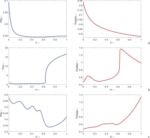\end{aligned}$ (1) ), Figure . It is apparent from Figure (a) that both prey and predator populations decrease with increase in fear factor. If fear effect is very high, the abundances of prey and predator become very low in the ecosystem. The refuge property of prey although increases prey density, but high refuge in prey population leads to decline in the predator density (see Figure (b)). We observe that moderate values of refuge can balance the prey as well as predator populations. Moreover, providing additional food to the predator population help to boost its density whereas diminish the prey with little bit fluctuations in the latter (see Figure (c)).

Figure 1. Variations of prey (first column) and predator (second column) densities in system (Equation1(1) $\begin{aligned} \frac{d N}{d t} & = \frac{r_{0} N}{1 + k P} - r_{1} N^{2} - \frac{α (1 - m P) N P}{θ + ξ η A + b (1 - m P) N + c P}, \\ \frac{d P}{d t} & = \frac{β {α (1 - m P) N + η A} P}{θ + ξ η A + b (1 - m P) N + c P} - d P . \end{aligned}$ (1) ) with respect to (a) k, (b) m and (c) A. Rest of the parameters are at the same values as in Table .

Figure 1. Variations of prey (first column) and predator (second column) densities in system (Equation1(1) dNdt=r0N1+kP−r1N2−α(1−mP)NPθ+ξηA+b(1−mP)N+cP,dPdt=β{α(1−mP)N+ηA}Pθ+ξηA+b(1−mP)N+cP−dP.(1) ) with respect to (a) k, (b) m and (c) A. Rest of the parameters are at the same values as in Table 1.

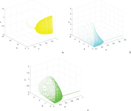
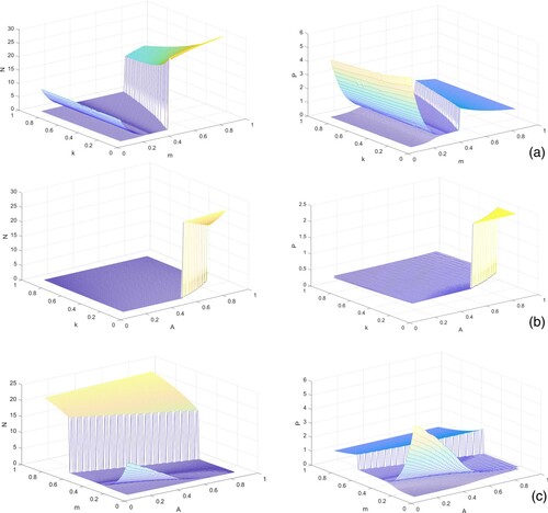
Next, we vary two parameters of system (Equation1(1) $\begin{aligned} \frac{d N}{d t} & = \frac{r_{0} N}{1 + k P} - r_{1} N^{2} - \frac{α (1 - m P) N P}{θ + ξ η A + b (1 - m P) N + c P}, \\ \frac{d P}{d t} & = \frac{β {α (1 - m P) N + η A} P}{θ + ξ η A + b (1 - m P) N + c P} - d P . \end{aligned}$ (1) ) at a time viz. $(m, k)$ , $(A, k)$ and $(A, m)$ , and see the evolutions of prey and predator populations, Figure . The pictures show surfaces representing the equilibrium level or the maximum and minimum values of prey and predator populations when they oscillate. These plots indicate that on varying m and k simultaneously, the prey population suddenly increases just after a fixed value of m. The predator population decreases on enhancement in prey refuge, but after a certain value of refuge coefficient, the predator population suddenly increase. We observe that although fear factor causes rapid decline in prey and predator populations, providing additional food accelerates their growths. Coupling A with m, we note that providing additional food fails to balance the growths in prey and predator whereas high refuge prevents the extinction of prey population.

Figure 2. Surface plots of prey (first column) and predator (second column) populations in system (Equation1(1) $\begin{aligned} \frac{d N}{d t} & = \frac{r_{0} N}{1 + k P} - r_{1} N^{2} - \frac{α (1 - m P) N P}{θ + ξ η A + b (1 - m P) N + c P}, \\ \frac{d P}{d t} & = \frac{β {α (1 - m P) N + η A} P}{θ + ξ η A + b (1 - m P) N + c P} - d P . \end{aligned}$ (1) ) with respect to (a) m and k, (b) A and k, and (c) A and m. Rest of the parameters are at the same values as in Table .

Figure 2. Surface plots of prey (first column) and predator (second column) populations in system (Equation1(1) dNdt=r0N1+kP−r1N2−α(1−mP)NPθ+ξηA+b(1−mP)N+cP,dPdt=β{α(1−mP)N+ηA}Pθ+ξηA+b(1−mP)N+cP−dP.(1) ) with respect to (a) m and k, (b) A and k, and (c) A and m. Rest of the parameters are at the same values as in Table 1.

7.2. Sensitivity analysis

In order to characterize the connection between the parameters of system (Equation1(1) $\begin{aligned} \frac{d N}{d t} & = \frac{r_{0} N}{1 + k P} - r_{1} N^{2} - \frac{α (1 - m P) N P}{θ + ξ η A + b (1 - m P) N + c P}, \\ \frac{d P}{d t} & = \frac{β {α (1 - m P) N + η A} P}{θ + ξ η A + b (1 - m P) N + c P} - d P . \end{aligned}$ (1) ) and its solutions, the differential sensitivity analysis of system (Equation1(1) $\begin{aligned} \frac{d N}{d t} & = \frac{r_{0} N}{1 + k P} - r_{1} N^{2} - \frac{α (1 - m P) N P}{θ + ξ η A + b (1 - m P) N + c P}, \\ \frac{d P}{d t} & = \frac{β {α (1 - m P) N + η A} P}{θ + ξ η A + b (1 - m P) N + c P} - d P . 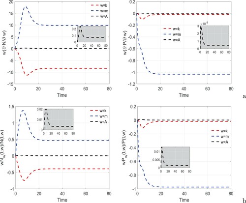\end{aligned}$ (1) ) is performed [Citation12, Citation47, Citation48]. The semi-relative and logarithmic sensitivity solutions with respect to three most sensitive relevant parameters k, m and A corresponding to the state variables (prey and predator) are computed. The former provide the amount the state will change when a parameter is doubled whereas the latter indicate percentage change in the state variable on doubling a model parameter. The sensitivities of model variables are plotted in Figure . In Figure (a), the semi relative sensitivity solutions are plotted. It is apparent from this figure that doubling the fear parameter k reduce the prey population by 8.3796 and the predator population by 0.0192 in 80 days. The prey population increases by 9.8826 whereas the predator population decreases by 1.0346 by doubling the refuge coefficient m in 80 days. Finally, doubling the parameter A causes increment in prey and predator populations by 0.0706 and 0.0004, respectively in 80 days. Note that both populations are least sensitive to the additional food for predator. This may be due to the fact that additional food to the predator contains low nutrients and also acquire less attention than focal prey. The fear of predator and the tendency of taking refuge highly influence the prey density. From Figure (b), which depicts logarithmic sensitivity solutions, it is evident that doubling the parameter k leads to 39.37% and 1.81% decrements in the prey and predator populations, respectively, in 80 days. On doubling the refuge parameter m, we observe 46.43% increase and 97.43% decrease in the prey and predator populations, respectively, in 80 days. The densities of prey and predator populations are boosted by 0.33% and 0.14%, respectively, in 80 days on doubling the value of A. As in the case of semi-relative sensitivity solutions, here also both the populations are least sensitive to the additional food, however, it fosters their growth. Both of these sensitivity solutions indicate that when fear of predator affects prey and hence the predator, prey refuge supports the survival of prey whereas providing additional food to the predator enhances the survivorships of prey and predator populations.

Figure 3. (a) Semi-relative sensitivity and (b) logarithmic sensitivity solutions of system (Equation1(1) $\begin{aligned} \frac{d N}{d t} & = \frac{r_{0} N}{1 + k P} - r_{1} N^{2} - \frac{α (1 - m P) N P}{θ + ξ η A + b (1 - m P) N + c P}, \\ \frac{d P}{d t} & = \frac{β {α (1 - m P) N + η A} P}{θ + ξ η A + b (1 - m P) N + c P} - d P . \end{aligned}$ (1) ) with respect to k, m and A. Parameters are at the same values as in Table except m = 0.9 and A = 0.7.

Figure 3. (a) Semi-relative sensitivity and (b) logarithmic sensitivity solutions of system (Equation1(1) dNdt=r0N1+kP−r1N2−α(1−mP)NPθ+ξηA+b(1−mP)N+cP,dPdt=β{α(1−mP)N+ηA}Pθ+ξηA+b(1−mP)N+cP−dP.(1) ) with respect to k, m and A. Parameters are at the same values as in Table 1 except m = 0.9 and A = 0.7.

7.3. Impacts of fear, refuge and additional food on the dynamics of system (1)

At first, we keep system (Equation1(1) $\begin{aligned} \frac{d N}{d t} & = \frac{r_{0} N}{1 + k P} - r_{1} N^{2} - \frac{α (1 - m P) N P}{θ + ξ η A + b (1 - m P) N + c P}, \\ \frac{d P}{d t} & = \frac{β {α (1 - m P) N + η A} P}{θ + ξ η A + b (1 - m P) N + c P} - d P . \end{aligned}$ (1) ) in the absence of fear, refuge and additional food, i.e. we set k = m = A = 0. We see the impact of theses three ecologically important parameters by introducing them in the system one-by-one. We find that for k = m = A = 0, the system (Equation1(1) $\begin{aligned} \frac{d N}{d t} & = \frac{r_{0} N}{1 + k P} - r_{1} N^{2} - \frac{α (1 - m P) N P}{θ + ξ η A + b (1 - m P) N + c P}, \\ \frac{d P}{d t} & = \frac{β {α (1 - m P) N + η A} P}{θ + ξ η A + b (1 - m P) N + c P} - d P . 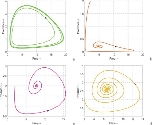\end{aligned}$ (1) ) is in oscillatory state (see Figure (a)) whereas the oscillations are terminated and the system returned to stable coexistence by incorporating only the fear factor (see Figure (b)) or prey refuge (see Figure (c)) or additional food (see Figure (d)). These results explored the stabilizing roles of fear [Citation69], prey refuge [Citation59] and additional food [Citation59] in a real predator–prey system.

Figure 4. Phase portraits of system (Equation1(1) $\begin{aligned} \frac{d N}{d t} & = \frac{r_{0} N}{1 + k P} - r_{1} N^{2} - \frac{α (1 - m P) N P}{θ + ξ η A + b (1 - m P) N + c P}, \\ \frac{d P}{d t} & = \frac{β {α (1 - m P) N + η A} P}{θ + ξ η A + b (1 - m P) N + c P} - d P . \end{aligned}$ (1) ) for $r_{0} = 0.5$ , $α = 0.36$ , $θ = 0.6$ and $β = 0.3$ . Rest of the parameters are at the same values as in Table except in (a) $r_{1} = 0.02$ , k = m = A = 0, (b) $r_{1} = 0.02$ , k = 10, m = A = 0, (c) $r_{1} = 0.02$ , m = 0.13, k = A = 0, and (d) $r_{1} = 0.02$ , $ξ = 0.3$ , $η = 0.4$ , A = 7, k = m = 0.

Figure 4. Phase portraits of system (Equation1(1) dNdt=r0N1+kP−r1N2−α(1−mP)NPθ+ξηA+b(1−mP)N+cP,dPdt=β{α(1−mP)N+ηA}Pθ+ξηA+b(1−mP)N+cP−dP.(1) ) for r0=0.5, α=0.36, θ=0.6 and β=0.3. Rest of the parameters are at the same values as in Table 1 except in (a) r1=0.02, k = m = A = 0, (b) r1=0.02, k = 10, m = A = 0, (c) r1=0.02, m = 0.13, k = A = 0, and (d) r1=0.02, ξ=0.3, η=0.4, A = 7, k = m = 0.

Now, we see the dynamics of system (Equation1(1) $\begin{aligned} \frac{d N}{d t} & = \frac{r_{0} N}{1 + k P} - r_{1} N^{2} - \frac{α (1 - m P) N P}{θ + ξ η A + b (1 - m P) N + c P}, \\ \frac{d P}{d t} & = \frac{β {α (1 - m P) N + η A} P}{θ + ξ η A + b (1 - m P) N + c P} - d P . \end{aligned}$ (1) ), where the fear, prey refuge and additional food are simultaneously present. The phase portraits of system (Equation1(1) $\begin{aligned} \frac{d N}{d t} & = \frac{r_{0} N}{1 + k P} - r_{1} N^{2} - \frac{α (1 - m P) N P}{θ + ξ η A + b (1 - m P) N + c P}, \\ \frac{d P}{d t} & = \frac{β {α (1 - m P) N + η A} P}{θ + ξ η A + b (1 - m P) N + c P} - d P . \end{aligned}$ (1) ) are depicted in Figure . We observe that the system exhibits limit cycle behaviour for higher values of fear factor whereas stability is achieved on decreasing the value of k. That is to say, fear effect destabilizes the system. In contrast, prey refuge and additional food stabilize the system, i.e. on increasing the value of any of them, the system returns to stable state from persistent oscillations which resemble the findings of Samanta et al. [Citation59]. In Figure , we draw bifurcation diagrams of system (Equation1(1) $\begin{aligned} \frac{d N}{d t} & = \frac{r_{0} N}{1 + k P} - r_{1} N^{2} - \frac{α (1 - m P) N P}{θ + ξ η A + b (1 - m P) N + c P}, \\ \frac{d P}{d t} & = \frac{β {α (1 - m P) N + η A} P}{θ + ξ η A + b (1 - m P) N + c P} - d P . \end{aligned}$ (1) ) with respect to the three interesting parameters, k, m and A. Rising of periodic solutions from stationary solution in N−P plane is apparent from Figure (a). This figure clearly shows the occurrence of Hopf-bifurcation on increasing the value of k. On the other hand, the existing periodic solution disappear and the system reaches to a stable state on increasing the value of m (see Figure (b)). Similar effect is observed for the additional food; increasing values of A evacuated the persistent oscillations and settle the system to a stable coexistence (see Figure (c)). Thus, fear of predator destabilizes the system through Hopf-bifurcation whereas prey refuge and additional food push back the system to stable state by terminating the limit cycle oscillations.

Figure 5. Phase portraits of system (Equation1(1) $\begin{aligned} \frac{d N}{d t} & = \frac{r_{0} N}{1 + k P} - r_{1} N^{2} - \frac{α (1 - m P) N P}{θ + ξ η A + b (1 - m P) N + c P}, \\ \frac{d P}{d t} & = \frac{β {α (1 - m P) N + η A} P}{θ + ξ η A + b (1 - m P) N + c P} - d P . \end{aligned}$ (1) ). Parameters are at the same values as in Table except in (a) m = 0.2, (b) k = 0.01, m = 0.2, $α = 0.35$ , $ξ = 0.03$ , (c) m = 0.4 and (d) m = 0.2, A = 0.5.

Figure 5. Phase portraits of system (Equation1(1) dNdt=r0N1+kP−r1N2−α(1−mP)NPθ+ξηA+b(1−mP)N+cP,dPdt=β{α(1−mP)N+ηA}Pθ+ξηA+b(1−mP)N+cP−dP.(1) ). Parameters are at the same values as in Table 1 except in (a) m = 0.2, (b) k = 0.01, m = 0.2, α=0.35, ξ=0.03, (c) m = 0.4 and (d) m = 0.2, A = 0.5.

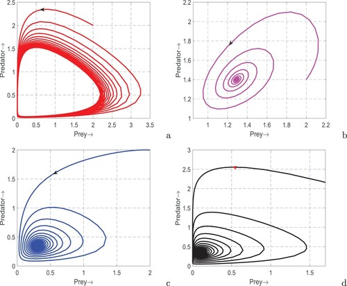
Figure 6. Bifurcation diagram of system (Equation1(1) $\begin{aligned} \frac{d N}{d t} & = \frac{r_{0} N}{1 + k P} - r_{1} N^{2} - \frac{α (1 - m P) N P}{θ + ξ η A + b (1 - m P) N + c P}, \\ \frac{d P}{d t} & = \frac{β {α (1 - m P) N + η A} P}{θ + ξ η A + b (1 - m P) N + c P} - d P . \end{aligned}$ (1) ) with respect to (a) k, (b) m and (c) A. Rest of the parameters are at the same values as in Table except in (a) $ξ = 0.03$ , $α = 0.35$ , m = 0.2 and (c) m = 0.2.

Figure 6. Bifurcation diagram of system (Equation1(1) dNdt=r0N1+kP−r1N2−α(1−mP)NPθ+ξηA+b(1−mP)N+cP,dPdt=β{α(1−mP)N+ηA}Pθ+ξηA+b(1−mP)N+cP−dP.(1) ) with respect to (a) k, (b) m and (c) A. Rest of the parameters are at the same values as in Table 1 except in (a) ξ=0.03, α=0.35, m = 0.2 and (c) m = 0.2.

7.4. Impact of delay in fear of predator

Here, we report the simulations performed to investigate the behaviour of delay differential equations (Equation12(12) $\begin{aligned} \frac{d N}{d t} & = \frac{r_{0} N}{1 + k P (t - τ)} - r_{1} N^{2} - \frac{α (1 - m P) N P}{θ + ξ η A + b (1 - m P) N + c P}, \\ \frac{d P}{d t} & = \frac{β {α (1 - m P) N + η A} P}{θ + ξ η A + b (1 - m P) N + c P} - d P . \end{aligned}$ (12) ). At first, we fix the values of parameters at which the system (Equation12(12) $\begin{aligned} \frac{d N}{d t} & = \frac{r_{0} N}{1 + k P (t - τ)} - r_{1} N^{2} - \frac{α (1 - m P) N P}{θ + ξ η A + b (1 - m P) N + c P}, \\ \frac{d P}{d t} & = \frac{β {α (1 - m P) N + η A} P}{θ + ξ η A + b (1 - m P) N + c P} - d P . \end{aligned}$ (12) ) is at stable state in the absence of time delay and gradually increase the magnitude of delay parameter τ. We plot the solution trajectories of system (Equation12(12) $\begin{aligned} \frac{d N}{d t} & = \frac{r_{0} N}{1 + k P (t - τ)} - r_{1} N^{2} - \frac{α (1 - m P) N P}{θ + ξ η A + b (1 - m P) N + c P}, \\ \frac{d P}{d t} & = \frac{β {α (1 - m P) N + η A} P}{θ + ξ η A + b (1 - m P) N + c P} - d P . \end{aligned}$ (12) ) in Figure . We see that at $τ = 4$ , the system shows limit cycle oscillations (see Figure (a)) whereas at $τ = 15$ , the system exhibits stable focus (see Figure (b)). On increasing the value of τ to $τ = 25$ , we observe that the system again showcases limit cycle oscillations (see Figure (c)). Finally, we pick $τ = 65$ and find that the dynamics of system (Equation12(12) $\begin{aligned} \frac{d N}{d t} & = \frac{r_{0} N}{1 + k P (t - τ)} - r_{1} N^{2} - \frac{α (1 - m P) N P}{θ + ξ η A + b (1 - m P) N + c P}, \\ \frac{d P}{d t} & = \frac{β {α (1 - m P) N + η A} P}{θ + ξ η A + b (1 - m P) N + c P} - d P . \end{aligned}$ (12) ) is chaotic (see Figure (d)); in the figure incommensurate limit cycles indicate the chaotic behaviour of the system [Citation33, Citation35]. Next, we set system (Equation12(12) $\begin{aligned} \frac{d N}{d t} & = \frac{r_{0} N}{1 + k P (t - τ)} - r_{1} N^{2} - \frac{α (1 - m P) N P}{θ + ξ η A + b (1 - m P) N + c P}, \\ \frac{d P}{d t} & = \frac{β {α (1 - m P) N + η A} P}{θ + ξ η A + b (1 - m P) N + c P} - d P . \end{aligned}$ (12) ) at oscillatory state in the absence of time delay and see the behaviour of system at $τ = 4$ , 15, 25 and 65 (see Figure ). It is apparent from the figure that the system exhibits limit cycle oscillations at $τ = 4$ and $τ = 15$ while at $τ = 65$ , the nature of system is chaotic. Interestingly, at $τ = 25$ , the system demonstrates periodic oscillations of period two. Thus, for a certain range of delay parameter, the peak of oscillations jumps between two values each year. To get a clear idea of stability change for increasing values of τ, we draw bifurcation diagram of system (Equation12(12) $\begin{aligned} \frac{d N}{d t} & = \frac{r_{0} N}{1 + k P (t - τ)} - r_{1} N^{2} - \frac{α (1 - m P) N P}{θ + ξ η A + b (1 - m P) N + c P}, \\ \frac{d P}{d t} & = \frac{β {α (1 - m P) N + η A} P}{θ + ξ η A + b (1 - m P) N + c P} - d P . \end{aligned}$ (12) ) for $τ \in (0, 70]$ , Figure . It is clear from the figure that for initial values of τ, the system shows limit cycle oscillations and becomes stable as τ increased. We observe several stability switches on gradual increase in the values of τ, and the system ultimately enters into chaotic regime through period doubling oscillations.

Figure 7. Time series of system (Equation12(12) $\begin{aligned} \frac{d N}{d t} & = \frac{r_{0} N}{1 + k P (t - τ)} - r_{1} N^{2} - \frac{α (1 - m P) N P}{θ + ξ η A + b (1 - m P) N + c P}, \\ \frac{d P}{d t} & = \frac{β {α (1 - m P) N + η A} P}{θ + ξ η A + b (1 - m P) N + c P} - d P . \end{aligned}$ (12) ) for different values of τ: (a) $τ = 4$ , (b) $τ = 15$ , (c) $τ = 25$ and (d) $τ = 65$ . Parameters are at the same values as in Table , and the initial conditions are chosen as (2, 1).

Figure 7. Time series of system (Equation12(12) dNdt=r0N1+kP(t−τ)−r1N2−α(1−mP)NPθ+ξηA+b(1−mP)N+cP,dPdt=β{α(1−mP)N+ηA}Pθ+ξηA+b(1−mP)N+cP−dP.(12) ) for different values of τ: (a) τ=4, (b) τ=15, (c) τ=25 and (d) τ=65. Parameters are at the same values as in Table 1, and the initial conditions are chosen as (2, 1).

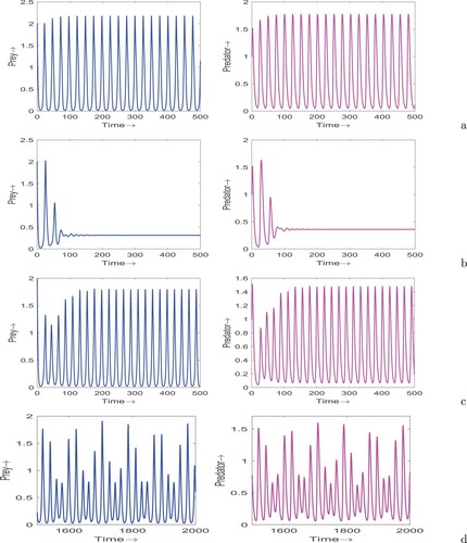
Figure 8. Time series of system (Equation12(12) $\begin{aligned} \frac{d N}{d t} & = \frac{r_{0} N}{1 + k P (t - τ)} - r_{1} N^{2} - \frac{α (1 - m P) N P}{θ + ξ η A + b (1 - m P) N + c P}, \\ \frac{d P}{d t} & = \frac{β {α (1 - m P) N + η A} P}{θ + ξ η A + b (1 - m P) N + c P} - d P . \end{aligned}$ (12) ) for different values of τ: (a) $τ = 4$ , (b) $τ = 15$ , (c) $τ = 25$ and (d) $τ = 65$ . Parameters are at the same values as in Figure (a), which shows oscillating behaviour of system (Equation1(1) $\begin{aligned} \frac{d N}{d t} & = \frac{r_{0} N}{1 + k P} - r_{1} N^{2} - \frac{α (1 - m P) N P}{θ + ξ η A + b (1 - m P) N + c P}, \\ \frac{d P}{d t} & = \frac{β {α (1 - m P) N + η A} P}{θ + ξ η A + b (1 - m P) N + c P} - d P . \end{aligned}$ (1) ).

Figure 8. Time series of system (Equation12(12) dNdt=r0N1+kP(t−τ)−r1N2−α(1−mP)NPθ+ξηA+b(1−mP)N+cP,dPdt=β{α(1−mP)N+ηA}Pθ+ξηA+b(1−mP)N+cP−dP.(12) ) for different values of τ: (a) τ=4, (b) τ=15, (c) τ=25 and (d) τ=65. Parameters are at the same values as in Figure 5(a), which shows oscillating behaviour of system (Equation1(1) dNdt=r0N1+kP−r1N2−α(1−mP)NPθ+ξηA+b(1−mP)N+cP,dPdt=β{α(1−mP)N+ηA}Pθ+ξηA+b(1−mP)N+cP−dP.(1) ).

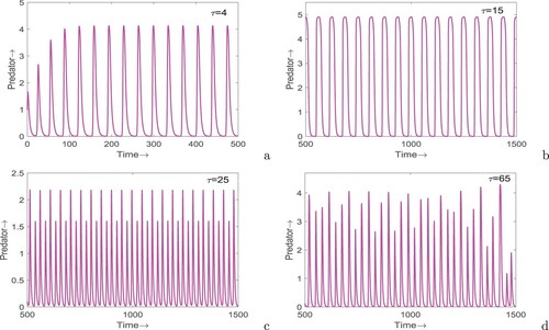
Figure 9. Bifurcation diagram of system (Equation12(12) $\begin{aligned} \frac{d N}{d t} & = \frac{r_{0} N}{1 + k P (t - τ)} - r_{1} N^{2} - \frac{α (1 - m P) N P}{θ + ξ η A + b (1 - m P) N + c P}, \\ \frac{d P}{d t} & = \frac{β {α (1 - m P) N + η A} P}{θ + ξ η A + b (1 - m P) N + c P} - d P . \end{aligned}$ (12) ) with respect to τ. Parameters are at the same values as in Table .

Figure 9. Bifurcation diagram of system (Equation12(12) dNdt=r0N1+kP(t−τ)−r1N2−α(1−mP)NPθ+ξηA+b(1−mP)N+cP,dPdt=β{α(1−mP)N+ηA}Pθ+ξηA+b(1−mP)N+cP−dP.(12) ) with respect to τ. Parameters are at the same values as in Table 1.

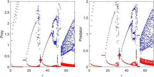
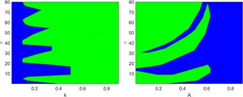
Figure demonstrates the stability regions of system (Equation12(12) $\begin{aligned} \frac{d N}{d t} & = \frac{r_{0} N}{1 + k P (t - τ)} - r_{1} N^{2} - \frac{α (1 - m P) N P}{θ + ξ η A + b (1 - m P) N + c P}, \\ \frac{d P}{d t} & = \frac{β {α (1 - m P) N + η A} P}{θ + ξ η A + b (1 - m P) N + c P} - d P . \end{aligned}$ (12) ) in (k,τ) and (A,τ) parametric planes. In the figures, blue regions represent the domains of stability for the coexistence equilibrium $E^{*}$ and green regions represent the domains of instability. From Figure (a), it is clear that for lower values of k, system (Equation12(12) $\begin{aligned} \frac{d N}{d t} & = \frac{r_{0} N}{1 + k P (t - τ)} - r_{1} N^{2} - \frac{α (1 - m P) N P}{θ + ξ η A + b (1 - m P) N + c P}, \\ \frac{d P}{d t} & = \frac{β {α (1 - m P) N + η A} P}{θ + ξ η A + b (1 - m P) N + c P} - d P . \end{aligned}$ (12) ) is always stable at the coexistence equilibrium for all values of time delay. Also, for higher values of k, the coexistence equilibrium is unstable irrespective of the values of τ. However, for moderate values of k, there exist stability switches for increasing values of τ. It is inferred from Figure (b) that for higher values of A, stable coexistence is achieved, i.e. delay does not affect stability behaviour of the system. On the other hand, for lower values of A, system switches its stability properties finite number of times with gradual increase in the values of time delay.

Figure 10. Stability regions for the system (Equation12(12) $\begin{aligned} \frac{d N}{d t} & = \frac{r_{0} N}{1 + k P (t - τ)} - r_{1} N^{2} - \frac{α (1 - m P) N P}{θ + ξ η A + b (1 - m P) N + c P}, \\ \frac{d P}{d t} & = \frac{β {α (1 - m P) N + η A} P}{θ + ξ η A + b (1 - m P) N + c P} - d P . \end{aligned}$ (12) ) in (a) $k - τ$ and (b) $A - τ$ planes. Here, blue regions represent the stable coexistence equilibrium for corresponding values of the parameters and green regions represent otherwise. Rest of the parameters are at the same values as in Table .

Figure 10. Stability regions for the system (Equation12(12) dNdt=r0N1+kP(t−τ)−r1N2−α(1−mP)NPθ+ξηA+b(1−mP)N+cP,dPdt=β{α(1−mP)N+ηA}Pθ+ξηA+b(1−mP)N+cP−dP.(12) ) in (a) k−τ and (b) A−τ planes. Here, blue regions represent the stable coexistence equilibrium for corresponding values of the parameters and green regions represent otherwise. Rest of the parameters are at the same values as in Table 1.

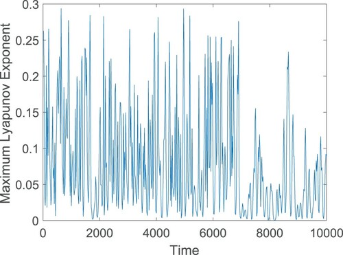
To confirm chaotic nature of system (Equation12(12) $\begin{aligned} \frac{d N}{d t} & = \frac{r_{0} N}{1 + k P (t - τ)} - r_{1} N^{2} - \frac{α (1 - m P) N P}{θ + ξ η A + b (1 - m P) N + c P}, \\ \frac{d P}{d t} & = \frac{β {α (1 - m P) N + η A} P}{θ + ξ η A + b (1 - m P) N + c P} - d P . \end{aligned}$ (12) ), we plot the maximum Lyapunov exponent of the system at $τ = 65$ by using the algorithm of [Citation56, Citation71], Figure . The maximum Lyapunov exponent has been proven to be most useful dynamical diagnostic for chaotic systems. It represents the average exponential rate of convergence/divergence of nearby orbits in the phase space. The idea of calculating its value is to follow two nearby orbits and calculate their average logarithmic rate of separation. Whenever they get too far apart, one of the orbits has to be moved back to the vicinity of the other along the line of separation. If the attractor is chaotic, the maximum Lyapunov exponent is positive; for a bifurcation point the maximum Lyapunov exponent is zero; the negative values of maximum Lyapunov exponent correspond to a fixed point/periodic attractor. To plot the maximum Lyapunov exponent, the delayed system (Equation12(12) $\begin{aligned} \frac{d N}{d t} & = \frac{r_{0} N}{1 + k P (t - τ)} - r_{1} N^{2} - \frac{α (1 - m P) N P}{θ + ξ η A + b (1 - m P) N + c P}, \\ \frac{d P}{d t} & = \frac{β {α (1 - m P) N + η A} P}{θ + ξ η A + b (1 - m P) N + c P} - d P . \end{aligned}$ (12) ) is first simulated, then by considering the time series solutions of each component of the system, the maximum Lyapunov exponent is computed. In Figure , the positive values of maximum Lyapunov exponent demonstrate the chaotic regime of system (Equation12(12) $\begin{aligned} \frac{d N}{d t} & = \frac{r_{0} N}{1 + k P (t - τ)} - r_{1} N^{2} - \frac{α (1 - m P) N P}{θ + ξ η A + b (1 - m P) N + c P}, \\ \frac{d P}{d t} & = \frac{β {α (1 - m P) N + η A} P}{θ + ξ η A + b (1 - m P) N + c P} - d P . \end{aligned}$ (12) ).

Figure 11. Maximum Lyapunov exponent of the system (Equation12(12) $\begin{aligned} \frac{d N}{d t} & = \frac{r_{0} N}{1 + k P (t - τ)} - r_{1} N^{2} - \frac{α (1 - m P) N P}{θ + ξ η A + b (1 - m P) N + c P}, \\ \frac{d P}{d t} & = \frac{β {α (1 - m P) N + η A} P}{θ + ξ η A + b (1 - m P) N + c P} - d P . \end{aligned}$ (12) ) at $τ = 65$ . Parameters are at the same values as in Table , and the initial conditions are chosen as (2, 1). In the figure, positive values of the maximum Lyapunov exponent confirm the occurrence of chaotic oscillation.

Figure 11. Maximum Lyapunov exponent of the system (Equation12(12) dNdt=r0N1+kP(t−τ)−r1N2−α(1−mP)NPθ+ξηA+b(1−mP)N+cP,dPdt=β{α(1−mP)N+ηA}Pθ+ξηA+b(1−mP)N+cP−dP.(12) ) at τ=65. Parameters are at the same values as in Table 1, and the initial conditions are chosen as (2, 1). In the figure, positive values of the maximum Lyapunov exponent confirm the occurrence of chaotic oscillation.

7.5. Impact of seasonality

Now, we incorporate seasonal variation in the fear parameter by considering $k (t)$ as a periodic function of time. The functional form of $k (t)$ is taken as $k (t) = k + k_{11} \sin (ω t)$ with period of one year. In this way, the periodic function in time encompasses both high and low seasons, that correspond to the periods in which $\sin (ω t)$ is positive and negative, respectively. The parameter $k_{11} (0 < k_{11} < k)$ controls the strength of the seasonal forcing. We investigate the impact of seasonality in the system with and without time delay. We plot solution trajectories for the predator population only (the prey population is found to exhibit similar behaviour), Figure . First, we fix $τ = 0$ in system (Equation51(51) $\begin{aligned} \frac{d N}{d t} & = \frac{r_{0} N}{1 + k (t) P (t - τ)} - r_{1} N^{2} - \frac{α (1 - m P) N P}{θ + ξ η A + b (1 - m P) N + c P}, \\ \frac{d P}{d t} & = \frac{β {α (1 - m P) N + η A} P}{θ + ξ η A + b (1 - m P) N + c P} - d P . \end{aligned}$ (51) ) and see how seasonal forcing is regulating the dynamics of system (see Figure ( a–c)). For a particular parameter set up, the autonomous system (Equation1(1) $\begin{aligned} \frac{d N}{d t} & = \frac{r_{0} N}{1 + k P} - r_{1} N^{2} - \frac{α (1 - m P) N P}{θ + ξ η A + b (1 - m P) N + c P}, \\ \frac{d P}{d t} & = \frac{β {α (1 - m P) N + η A} P}{θ + ξ η A + b (1 - m P) N + c P} - d P . \end{aligned}$ (1) ) shows stable focus whereas the non-autonomous system (Equation51(51) $\begin{aligned} \frac{d N}{d t} & = \frac{r_{0} N}{1 + k (t) P (t - τ)} - r_{1} N^{2} - \frac{α (1 - m P) N P}{θ + ξ η A + b (1 - m P) N + c P}, \\ \frac{d P}{d t} & = \frac{β {α (1 - m P) N + η A} P}{θ + ξ η A + b (1 - m P) N + c P} - d P . \end{aligned}$ (51) ) without delay shows periodic solution (see Figure (a)). Figure (b) shows that solutions initiating from three distinct points ultimately go to a unique periodic solution, i.e. the positive periodic solution is globally attractive. It is apparent from Figure (c ,d) that when systems (Equation1(1) $\begin{aligned} \frac{d N}{d t} & = \frac{r_{0} N}{1 + k P} - r_{1} N^{2} - \frac{α (1 - m P) N P}{θ + ξ η A + b (1 - m P) N + c P}, \\ \frac{d P}{d t} & = \frac{β {α (1 - m P) N + η A} P}{θ + ξ η A + b (1 - m P) N + c P} - d P . \end{aligned}$ (1) ) and (Equation12(12) $\begin{aligned} \frac{d N}{d t} & = \frac{r_{0} N}{1 + k P (t - τ)} - r_{1} N^{2} - \frac{α (1 - m P) N P}{θ + ξ η A + b (1 - m P) N + c P}, \\ \frac{d P}{d t} & = \frac{β {α (1 - m P) N + η A} P}{θ + ξ η A + b (1 - m P) N + c P} - d P . \end{aligned}$ (12) ) show limit cycle oscillations, the non-autonomous system (Equation51(51) $\begin{aligned} \frac{d N}{d t} & = \frac{r_{0} N}{1 + k (t) P (t - τ)} - r_{1} N^{2} - \frac{α (1 - m P) N P}{θ + ξ η A + b (1 - m P) N + c P}, \\ \frac{d P}{d t} & = \frac{β {α (1 - m P) N + η A} P}{θ + ξ η A + b (1 - m P) N + c P} - d P . \end{aligned}$ (51) ) shows higher periodicity. Figure (e) depicts that chaotic nature of system (Equation12(12) $\begin{aligned} \frac{d N}{d t} & = \frac{r_{0} N}{1 + k P (t - τ)} - r_{1} N^{2} - \frac{α (1 - m P) N P}{θ + ξ η A + b (1 - m P) N + c P}, \\ \frac{d P}{d t} & = \frac{β {α (1 - m P) N + η A} P}{θ + ξ η A + b (1 - m P) N + c P} - d P . \end{aligned}$ (12) ) turns into higher periodic behaviour when seasonal effect is introduced in the fear factor. For a particular parameter set up, the chaotic behaviour of system (Equation12(12) $\begin{aligned} \frac{d N}{d t} & = \frac{r_{0} N}{1 + k P (t - τ)} - r_{1} N^{2} - \frac{α (1 - m P) N P}{θ + ξ η A + b (1 - m P) N + c P}, \\ \frac{d P}{d t} & = \frac{β {α (1 - m P) N + η A} P}{θ + ξ η A + b (1 - m P) N + c P} - d P . 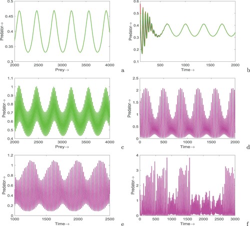\end{aligned}$ (12) ) remain unchanged although the fear parameter vary seasonally (see Figure (f)).

Figure 12. Time series solutions of system (Equation51(51) $\begin{aligned} \frac{d N}{d t} & = \frac{r_{0} N}{1 + k (t) P (t - τ)} - r_{1} N^{2} - \frac{α (1 - m P) N P}{θ + ξ η A + b (1 - m P) N + c P}, \\ \frac{d P}{d t} & = \frac{β {α (1 - m P) N + η A} P}{θ + ξ η A + b (1 - m P) N + c P} - d P . \end{aligned}$ (51) ) in the absence as well as presence of time delay. Parameters are at the same values as in Table , $ω = 2 π / 365$ except in (a) $k_{11} = 0.45$ , A = 0.6, $τ = 0$ , (b) $k_{11} = 0.45$ , m = 0.2, A = 0.6, $τ = 0$ , (c) k = 0.8, $k_{11} = 0.4$ , $α = 0.35$ , m = 0.2, $ξ = 0.03$ , $τ = 0$ , (d) $k_{11} = 0.4$ , $τ = 4$ , (e) k = 0.4, $k_{11} = 0.35$ , $τ = 65$ and (f) $k_{11} = 0.4$ , m = 0.2, $τ = 65$ .

Figure 12. Time series solutions of system (Equation51(51) dNdt=r0N1+k(t)P(t−τ)−r1N2−α(1−mP)NPθ+ξηA+b(1−mP)N+cP,dPdt=β{α(1−mP)N+ηA}Pθ+ξηA+b(1−mP)N+cP−dP.(51) ) in the absence as well as presence of time delay. Parameters are at the same values as in Table 1, ω=2π/365 except in (a) k11=0.45, A = 0.6, τ=0, (b) k11=0.45, m = 0.2, A = 0.6, τ=0, (c) k = 0.8, k11=0.4, α=0.35, m = 0.2, ξ=0.03, τ=0, (d) k11=0.4, τ=4, (e) k = 0.4, k11=0.35, τ=65 and (f) k11=0.4, m = 0.2, τ=65.

8. Conclusion

In every ecological system, prey populations are always threatened by predators and perceived predation risk. The fear of predation alters the behaviour of prey population. In predator–prey systems, the prey population shows a variety of different defense mechanisms to escape from predation; one of them is prey refuge, which decreases the predation rate. In contrast, the additional food always provides benefits to the predator population and helps the predators to persist in the system. In this paper, we have studied the combined effects of fear, refuge and additional food on the interacting dynamics of a predator–prey system. Our sensitivity results showed that both prey and predator populations decrease with increase in the fear factor, and the abundances are too low for higher level of fear of predator. However, the joint effects of reduction in prey refuge and the presence of appropriate amount of additional food can control the prey population. Numerical results showed that fear induces oscillation in the system, which can be terminated by increasing the refuge coefficient or amount of additional food to the predator. However, if the system exhibits persistent oscillations in the absence of fear, prey refuge and additional food for the predator, then stability can be regained by including the role of any of these three ecological factors. The existence of limit cycles in predator–prey systems can be used to explain many real-world oscillatory phenomena, such as the Canadian lynx snowshoe hare 10-year cycles.

Further, we have incorporated time delay involved in the process of perceiving predator's signals through chemical and/or vocal cues and the changes in life history and behavioural responses in the prey population. We have analysed the delayed system for the existence of Hopf bifurcation by taking time delay as a bifurcation parameter. We also obtained analytical conditions determining nature of the bifurcating periodic solutions. Moreover, sufficient conditions are derived under which the coexistence equilibrium is globally asymptotically stable in the presence of time delay. We gradually increase the delay parameter and observed that our delayed system experiences multiple stability switches through chaotic dynamics; for larger values of time delay, the system remains chaotic. Ecologically, presence of chaos affects ecosystem features such as predictability, species persistence [Citation4], and biodiversity [Citation38]. Moreover, we observed that presence of delay in fear of predator has no effect on the system's dynamics if the level of fear is too low or too high. However, for moderate level of fear or additional food, the system experienced finitely many stability switches on increasing time lag in the fear of predator.

Furthermore, we consider seasonal variation in the level of fear, and assume that it is periodic function of time with a period of one year. We saw the impact of seasonal changes in fear effect on the dynamics of systems with and without time delay. Our non-autonomous system exhibits positive periodic solution for the set of parameter values at which the corresponding autonomous system is stable. We showed that the positive periodic solution is globally attractive. However, if the autonomous system with or without time delay shows limit cycle oscillations, the non-autonomous counterpart generates higher periodic solutions. The outcomes of the present investigation are very important for understanding complex behaviours of dynamical systems, and have wide spread applications in conservation biology.

Acknowledgments

The authors thank the associate editor and anonymous reviewers for their valuable comments, which contributed to the improvement in the presentation of the paper.

Disclosure statement

No potential conflict of interest was reported by the author(s).

Additional information

Funding

Nazmul Sk acknowledges financial support from University Grants Commissions, New Delhi, India in the form of Junior Research Fellowship (F.No. 16- 6(DEC.2018)/2019, NET/CSIR, No.F.4-2/2006 (BSR)/MA/17-18/0021). The research of Samares Pal is partially supported by Science and Engineering Research Board, Government of India [grant number No. CRG/2019/003248, MTR/2020/000542].

References

S. Ahmad, On the nonautonomous Volterra–Lotka competition equations, Proc. Amer. Math. Soc. 117 (1993), pp. 199–204.
Web of Science ®Google Scholar
S. Ahmad, Extinction of species in nonautonomous Lotka–Volterra systems, Proc. Amer. Math. Soc. 127 (1999), pp. 2905–2910.
Web of Science ®Google Scholar
S. Ahmad and A.C. Lazer, Average conditions for global asymptotic stability in a nonautonomous Lotka–Volterra system, Nonlinear Anal. Theor. Methods Appl. 40 (2000), pp. 37–49.
Web of Science ®Google Scholar
J.C. Allen, W.M. Schaffer, and D. Rosko, Chaos reduces species extinctions by amplifying local population noise, Nature. 364 (1993), pp. 229–232.
PubMed Web of Science ®Google Scholar
K.B. Altendorf, J.W. Laundré, C.A. López González, and J.S. Brown, Assessing effects of predation risk on foraging behavior of mule deer, J. Mammal. 82(2) (2001), pp. 430–439.
Web of Science ®Google Scholar
R. Arditi and H. Saiah, Empirical evidence of the role of heterogeneity in ratio-dependent consumption, Ecology 73(5) (1992), pp. 1544–1551.
Web of Science ®Google Scholar
Y. Bai and Y. Li, Stability and Hopf-bifurcation for a stage-structured predator–prey model incorporating refuge for prey and additional food for predator, Adv. Differ. Equ. 42 (2019), pp. 2019.
Google Scholar
J.R. Beddington, Mutual interference between parasites or predators and its effect on searching efficiency, J. Anim. Ecol. 44 (1975), pp. 331–340.
Web of Science ®Google Scholar
E. Beretta and Y. Kuang, Convergence results in a well known delayed predator–prey system, J. Math. Anal. Appl. 204 (1996), pp. 840–853.
Web of Science ®Google Scholar
S. Biswas, S. Samanta, and J. Chattopadhyay, A model based theoretical study on cannibalistic prey–predator system with disease in both populations, Diff. Equs. Dyn. Syst. 23 (2015), pp. 327–370.
Web of Science ®Google Scholar
S. Biswas, P.K. Tiwari, and S. Pal, Delay-induced chaos and its possible control in a seasonally forced eco-epidemiological model with fear effect and predator switching, Nonlinear Dyn. 104(3) (2021), pp. 2901–2930.
Web of Science ®Google Scholar
D.M. Bortz and P.W. Nelson, Sensitivity analysis of a nonlinear lumped parameter model of HIV infection dynamics, Bull. Math. Biol. 66 (2004), pp. 1009–1026.
PubMed Web of Science ®Google Scholar
U. Candolin, Reproduction under predation risk and the trade-off between current and future reproduction in the threespine stickleback, Proc. R. Soc. Lond. [Biol.] 265(1402) (1998), pp. 1171–1175.
Google Scholar
R.S. Cantrell and C. Cosner, On the dynamics of predator–prey models with the Beddington–DeAngelis functional response, J. Math. Anal. Appl. 257 (2001), pp. 206–222.
Web of Science ®Google Scholar
S. Chakroborty, P.K. Tiwari, S.K. Sasmal, S. Biswas, S. Bhattacharya, and J. Chattopadhyay, Interactive effects of prey refuge and additional food for predator in diffusive predator–prey system, Appl. Math. Model. 47 (2017), pp. 128–140.
Web of Science ®Google Scholar
J.H. Connell, A predator–prey system in the marine intertidal region. I, Balanus glandula and several predatory species of Thais, Ecol. Monogr. 40(1) (1970), pp. 49–78.
Web of Science ®Google Scholar
S. Creel, D. Christianson, S. Liley, and J.A. Winnie, Predation risk affects reproductive physiology and demography of elk, Science. 315(5814) (2007), pp. 960–960.
PubMed Web of Science ®Google Scholar
J.M. Cushing, Periodic time dependent predator–prey systems, SIAM J. Appl. Math. 32 (1997), pp. 82–95.
Google Scholar
A. Das and G.P. Samanta, Modeling the fear effect on a stochastics prey–predator system with additional food for the predator, J. Phys. A. Math. Theor. 51(46) (2018), pp. 465601.
Web of Science ®Google Scholar
A. Das and G.P. Samanta, A prey-predator model with refuge for prey and additional food for predator in a fluctuating environment, Phys. A. 538 (2020), p. 122844.
Web of Science ®Google Scholar
D.L. DeAngelis, R.A. Goldstein, and R.V. O'Neill, A model for trophic interaction, Ecology 56 (1975), pp. 881–892.
Web of Science ®Google Scholar
D.T. Dimitrov and H.V. Kojouharov, Complete mathematical analysis of predator–prey models with linear prey growth and Beddington–DeAngelis functional response, Appl. Math. Comput. 162(2) (2005), pp. 523–538.
Web of Science ®Google Scholar
R.A. Dolbeer and W.R. Clark, Population ecology of snowshoe hares in the central rocky mountains, J. Wildl. Manag. 39(3) (1975), pp. 535–549.
Web of Science ®Google Scholar
P.M. Dolman, The intensity of interference varies with resource density: Evidence from a field study with snow buntings, Plectrophenax Nivalis, Oecologia 102(4) (1995), pp. 511–514.
PubMed Web of Science ®Google Scholar
K.H. Elliott, Experimental evidence for within- and cross-seasonal effects of fear on survival and reproduction, J. Anim. Ecol. 85 (2016), pp. 507–515.
PubMed Web of Science ®Google Scholar
M. Fan and Y. Kuang, Dynamics of a nonautonomous predator–prey system with the Beddington–DeAngelis functional response, J. Math. Anal. Appl. 295(1) (2004), pp. 15–39.
Web of Science ®Google Scholar
R.E. Gaines and J.L. Mawhin, Coincidence Degree and Nonlinear Differential Equations, Springer-Verlag, Berlin, 1977.
Google Scholar
G.F. Gause, The Struggle for Existence, The Williams and Wilkins Comapny, Baltimore, 1934.
Google Scholar
K. Ghosh, S. Biswas, S. Samanta, P. K. Tiwari, A. S. Alshomrani, and J. Chattopadhyay, Effect of multiple delays in an eco-epidemiological model with strong Allee effect, Int. J. Bifur. Chaos. 27(11) (2017), p. 1750167.
Web of Science ®Google Scholar
J. Ghosh, B. Sahoo, and S. Poria, Prey–predator dynamics with prey refuge providing additional food to predator, Chaos Solit. Fract. 96 (2017), pp. 110–119.
Web of Science ®Google Scholar
K. Gopalsamy, Stability and Oscillations in Delay Differential Equations of Population Dynamics, Kluwer Academic Publishers, Boston, 1992.
Google Scholar
A.L. Greggor, J.W. Jolles, A. Thornton, and N.S. Clayton, Seasonal changes in neophobia and its consistency in rooks: The effect of novelity type and dominance position, Anim. Behav. 121 (2016), pp. 11–20.
PubMed Web of Science ®Google Scholar
J. Guckenheimer and P. Holmes, Nonlinear Oscillations, Dynamical Systems, and Bifurcations of Vector Fields, Vol. 42, Springer Science & Business Media, New York, 2013.
Google Scholar
B. Hassard, D. Kazarinof, and Y. Wan, Theory and Applications of Hopf Bifurcation, Cambridge University Press, Cambridge, 1981.
Google Scholar
A. Hastings and T. Powell, Chaos in a three-species food chain, Ecology. 72(3) (1991), pp. 896–903.
Web of Science ®Google Scholar
M. Hossain, N. Pal, and S. Samanta, Impact of fear on an eco-epidemiological model, Chaos Solit. Fract. 134 (2020), pp. 109718.
Google Scholar
M. Hossain, N. Pal, S. Samanta, and J. Chattopadhyay, Fear induced stabilization in an intraguild predation model, Int. J. Bifur. Chaos. 30(04) (2020), pp. 2050053.
Google Scholar
J. Huisman and F. Weissing, Biodiversity of plankton by species oscillations and chaos, Nature 402 (1999), pp. 407–411.
Web of Science ®Google Scholar
A. Kumar and B. Dubey, Modeling the effect of fear in a prey–predator system with prey refuge and gestation delay, Int. J. Bifur. Chaos. 29(14) (2019), pp. 1950195.
Google Scholar
V. Kumar and N. Kumari, Controlling chaos in three species food chain model with fear effect, Math. Biosci. Eng. 5(2) (2020), pp. 828–842.
Google Scholar
V. Lakshmikantham, S. Leela, and A.A. Martynyuk, Stability Analysis of Nonlinear Systems, Marcel Dekker, Inc., New York/Basel, 1989.
Google Scholar
Q. Liu and D. Jiang, Influence of the fear factor on the dynamics of a stochastic predator–prey model, Appl. Math. Lett. 112 (2021), pp. 106756.
Google Scholar
M. Liu and K. Wang, Global stability of a nonlinear stochastic predator–prey system with Beddington–DeAngelis functional response, Commun. Nonlinear Sci. Numer. Simul. 16(3) (2011), pp. 1114–1121.
Web of Science ®Google Scholar
T.T. Macan, A twenty-one-year study of the water-bugs in a moorland fishpond, J. Anim. Ecol. 45(3) (1976), pp. 913–922.
Web of Science ®Google Scholar
A. Mandal, P.K. Tiwari, S. Samanta, E. Venturino, and S. Pal, A nonautonomous model for the effect of environmental toxins on plankton dynamics, Nonlinear Dyn. 99(4) (2020), pp. 3373–3405.
Web of Science ®Google Scholar
A.K. Misra and B. Dubey, A ratio-dependent predator–prey model with delay and harvesting, J. Biol. Syst. 18(02) (2010), pp. 437–453.
Google Scholar
A.K. Misra, P.K. Tiwari, and E. Venturino, Modeling the impact of awareness on the mitigation of algal bloom in a lake, J. Biol. Phys. 42(1) (2016), pp. 147–165.
PubMed Web of Science ®Google Scholar
A.K. Misra and M. Verma, Modeling the impact of mitigation options on methane abatement from rice fields, Mitig. Adapt. Strate. Glob. Chang. 19(7) (2014), pp. 927–945.
Web of Science ®Google Scholar
H. Molla, M.S. Rahman, and S. Sarwardi, Dynamics of a predator–prey model with Holling type II functional response incorporating a prey refuge depending on both the species, Int. J. Nonlin. Sci. Numer. Simul. 20(1) (2019), pp. 89–104.
Web of Science ®Google Scholar
S. Mondal, A. Maiti, and G.P. Samanta, Effects of fear and additional food in a delayed predator–prey model, Biophys. Rev. Lett. 13(04) (2018), pp. 157–177.
Google Scholar
S. Mondal and G.P. Samanta, Dynamics of a delayed predator–prey interaction incorporating non-linear prey refuge under the influence of fear effect and additional food, J. Phys. A. Math. Theor. 53(29) (2020), pp. 295601.
Google Scholar
S. Pal, S. Majhi, S. Mandal, and N. Pal, Role of fear in a predator–prey model with Beddington–DeAngelis functional response, Z. Naturforschung A. 74(7) (2019), pp. 581–595.
Google Scholar
P. Panday, N. Pal, S. Samanta, and J. Chattopadhyay, Stability and bifurcation analysis of a three-species food chain model with fear, Int. J. Bifur. Chaos 28(01) (2018), p. 1850009.
Google Scholar
P. Panday, N. Pal, S. Samanta, and J. Chattopadhyay, A three species food chain model with fear induced tropic cascade, Int. J. Appl. Comput. Math. 5(4) (2019), pp. 1242.
Google Scholar
P. Panday, S. Samanta, N. Pal, and J. Chattopadhyay, Delay induced multiple stability switch and chaos in a predator–prey model with fear effect, Math. Comput. Simul. 172 (2020), pp. 134–158.
Web of Science ®Google Scholar
T. Park, A Matlab version of the Lyapunov exponent estimation algorithm of Wolf et al. Physica 16d, 1985, 2014. Available from: https://www.mathworks.com/matlabcentral/fileexchange/48084-lyapunov-exponent-estimation-from-a-time-series-documentation-added.
Google Scholar
L. Perko, Differenetial Equations and Dynamical Systems, 3rd ed., Springer-Verlag, New York, 2000.
Google Scholar
J. Roy and S. Alam, Fear factor in a prey–predator system in deterministic and stochastic environment, Phys. A Stat. Mech. Appl. 541 (2020), pp. 123359.
Google Scholar
S. Samanta, R. Dhar, I.M. Elmojtaba, and J. Chattopadhyay, The role of additional food in a predator–prey model with a prey refuge, J. Biol. Syst. 24(02/03) (2016), pp. 345–365.
Google Scholar
A. Sarkar, P.K. Tiwari, F. Bona, and S. Pal, Chaos in a nonautonomous model for the interactions of prey and predator with effect of water level fluctuation, J. Biol. Syst. 28(4) (2020), pp. 865–900.
Web of Science ®Google Scholar
A. Sha, S. Samanta, M. Martcheva, and J. Chattopadhyay, Backward bifurcation, oscillation and chaos in an eco-epidemilogical model with fear effect, J. Biol. Dyn. 13(8) (2019), pp. 301–327.
PubMedGoogle Scholar
N. Sk, P.K. Tiwari, Y. Kang, and S. Pal, A nonautonomous model for the interactive effects of fear, refuge and additional food in a prey–predator system, J. Biol. Syst. 29(1) (2021), pp. 107–145.
Google Scholar
N. Sk, P.K. Tiwari, and S. Pal, A delay nonautonomous model for the impacts of fear and refuge in a three species food chain model with hunting cooperation, Math. Comput. Simul. 192 (2022), pp. 136–166.
Google Scholar
G.T. Skalski and J.F. Gilliam, Functional responses with predator interference: Viable alternatives to the Holling type II model, Ecology 82 (2001), pp. 3083–3092.
Web of Science ®Google Scholar
V. Tiwari, J.P. Tripathi, S. Mishra, and R.K. Upadhyay, Modelling the fear effect and stability of non-equilibrium patterns in mutually interferring predator–prey system, Appl. Math. Comput. 371 (2020), pp. 124948.
Google Scholar
R.K. Upadhyay and S. Mishra, Population dynamic consequences of fearful prey in a spatiotemporal predator–prey system, Math. Biosci. Eng. 16(1) (2019), pp. 338–372.
Web of Science ®Google Scholar
J. Wang, Y. Cai, S. Fu, and W. Wang, The effect of the fear factor on the dynamics of predator–prey model incorporating the prey refuge, Chaos. 29 (2019), pp. 083109.
Google Scholar
X. Wang, Z. Du, and J. Liang, Existence and global attractivity of positive periodic solution to a Lotka–Volterra model, Nonlinear Anal. Real World Appl. 11 (2010), pp. 4054–4061.
Web of Science ®Google Scholar
X. Wang, L. Zanette, and X. Zou, Modelling the fear effect in predator–prey interactions, J. Math. Biol. 73 (2016), pp. 1179–1204.
PubMed Web of Science ®Google Scholar
C. M Williams, G. J Ragland, G. Betini, L. B Buckley, Z. A Cheviron, K. Donohue, J. Hereford, M. M Humphries, S. Lisovski, K. E Marshall, P. S Schmidt, K. S Sheldon, Ø. Varpe, and M. E Visser, Understanding evolutionary impacts of seasonality: An introduction to the symposium, Integr. Comp. Biol. 57(5) (2017), pp. 921–933.
PubMed Web of Science ®Google Scholar
A. Wolf, J.B. Swift, H.L. Swinney, and J.A. Vastano, Determining Lyapunov exponents from a time series, Phys. D. 16(3) (1985), pp. 285–317.
Web of Science ®Google Scholar
Y. Xia and S. Yuan, Survival analysis of a stochastic predator–prey model with prey refuge and fear effect, J. Biol. Dyn. 14(1) (2020), pp. 871–892.
PubMed Web of Science ®Google Scholar
F.B. Yousef, A. Yousef, and C. Maji, Effects of fear in a fractional-order predator–prey system with predator density-dependent prey mortality, Chaos Solit. Fract. 145 (2021), pp. 110711.
Google Scholar
L.Y. Zanette, A.F. White, M.C. Allen, and M. Clinchy, Perceived predation risk reduces the number of offspring songbirds produce per year, Science 334 (2011), pp. 1398–1401.
PubMed Web of Science ®Google Scholar
H. Zhang, Y. Cai, S. Fu, and W. Wang, Impact of the fear effect in a prey–predator model incorporating a prey refuge, Appl. Math. Comput. 356 (2019), pp. 328–337.
Web of Science ®Google Scholar

A delay non-autonomous model for the combined effects of fear, prey refuge and additional food for predator

Abstract

1. Introduction

2. The mathematical model

3. Mathematical analysis of system (1)