
 ?Mathematical formulae have been encoded as MathML and are displayed in this HTML version using MathJax in order to improve their display. Uncheck the box to turn MathJax off. This feature requires Javascript. Click on a formula to zoom.
Abstract
This note provides an elementary derivation of the basic reproduction number and the effective reproduction number from the discrete Kermack–McKendrick epidemic model. The derived formulae match those derived from the continuous version of the model; however, the derivation from discrete model is a bit more intuitive. The MATLAB functions for its calculation are given. A real case example is considered and the results are compared with those obtained by the R0 and the EpiEstim software packages.
Introduction
In addition to the incidence and prevalence [Citation1,Citation2], the reproductive number is one of the most useful epidemiologic metrics for monitoring and controlling the development of an epidemic [Citation3–9]. While the incidence and prevalence tell us something about the size of the epidemic, the reproduction number informs us of its spread rate.
There are two kinds of reproduction numbers: the basic reproduction number, , and the effective (or time-varying) reproduction number,
.
is defined only at the beginning of an outbreak and ‘represents the number of secondary cases that one case can produce if introduced to a susceptible population’ [Citation10].
is defined over the entire period of an epidemic and represents ‘the average number of secondary infectious produced by typical infective during the entire period of infectiousness’ [Citation11]. Neither
nor
is a natural constant, because their value depends on the epidemic model used. For various models used for analyzing properties and for calculation of
, see [Citation12–24]. For properties and calculation of R, see [Citation25–30]. For critical consideration of
, see [Citation31] and references therein.
We first review the formulas for calculating and
based on the continuous Kermack and McKendrick epidemic model [Citation32,Citation33]. Heesterbeek and Dietz [Citation14] used the following form of the model
(1)
(1) where
is the incidence rate,
is the density of susceptibles in the population,
is excepted infectivity of a person with infection age
. They define
(2)
(2) and derived the following expressions
(3)
(3) where
is the initial density of the susceptible population and
is the natural growth rate. From these expressions, Wallinga and Lipsitch [Citation34], by introducing generation time distribution
(4)
(4) deduce a formula for calculation of
, which has the form
(5)
(5)
For practical calculation, they offer a discrete version of this formula implemented in the R0 package [Citation35].
It seems that Fraser [Citation26] was the first who deduce a general formula for calculation of from the Kermack and McKendrick model. He starts with a generalization of Equation (1) in the form of a continuous renewal equation
(6)
(6) where
is the transmissibility. He defines the case reproduction number
as ‘the average number of people someone infected at time t can expect to infect’, thus
(7)
(7) and the instantaneous reproduction number
as ‘the average number of people someone infected at time t could expect to infect should conditions remain unchanged’, expressed by the formula,
(8)
(8)
Assuming that can be factorized as
(9)
(9) he deduces
(10)
(10) and from this formula, a discrete version of the formula for calculation of
and
. The method was implemented in the EpiEstim package [Citation36,Citation37].
We will follow the above ideas, but, unlike the authors mentioned, we will derive formulas for calculating the reproduction number from the discrete form of the Kermack–McKendrick epidemic model. In particular, this derivation does not need the factorization assumption Equation (9), and the derivation of the formula (4) for generation time is a bit more intuitive. For other discrete models, see [Citation38] and references therein.
Kermack–McKendrick epidemic model
Let denote the number of infectious peoples at calendar time n and infection-age k. Let
be the number of peoples who became infected at the calendar time n. We call them nth generation. The transition process of the epidemic for the nth generation is as follows
and the whole epidemic process may be schematically represented in this way [Citation32,Citation33]:
Here, t is calendar time and is the infection age.
Two hypotheses govern the epidemic process. The first one is that a decline in the number of infected in nth generation depends only on age. Thus, we have
(11)
(11) where
is the removal rate. From this, it follows that
(12)
(12)
A non-dimensional parameter can be interpreted as the probability that an individual of age k is still infectious [Citation3,Citation19].
Before stating the second hypothesis, we decompose to local
and imported
cases [Citation37]:
(13)
(13)
The second hypothesis assumes that is proportional to the number of contacts each generation has with all susceptible left in time interval n [Citation32]:
(14)
(14) where
is the infective rate at age
and
is the number of susceptible individuals at the time interval
. Using Equations (12), (13) and (14), we obtain
(15)
(15) where
is the infectivity at age
[Citation19,Citation39]; i.e. the number of new infectives in unit time per ineffective contact. Note that the Equation (15) assumes that ‘an individual is not infective at the moment of infection’ [Citation32], so, starting at the 0th generation, we assume
(16)
(16) where
is a constant and
the number of infected individuals initially. Equations (16) and (15) represent the discrete Kermack–McKendrick epidemic model that we will use to derive the formulas for calculating
and
.
Basic reproduction number
To derive the formula for calculation of , we start with the epidemic process for 0th generation:
Thus, the number of infectious individuals of 0th generation at each time interval is, by Equation (12),
and the new infected individuals produced by these infectives are, by Equation (15),
(17)
(17)
The total number of secondary infections produced by 0th generation is thus
(18)
(18)
If
(19)
(19) i.e. the susceptible population remains the same (which would literally mean that the newly infected individual is immediately removed and replaced by a new susceptible, but practically that the population is large), and we set
and
in Equation (16), then
, and thus, by definition[Citation14],
(20)
(20)
This is a discrete form of Equation (2).
Note. We could set and
, but we want to keep
in the expression in order to use an empirical law for I, which depends on the initial condition
.
The sequence of infected individuals produced by one infective in a completely susceptible population is thus, by Equation (17),
(21)
(21)
Dividing each term of this sequence by Equation (20), we obtain the sequence of the fractions of infected produced by one infected case:
(22)
(22) where
(23)
(23)
Thus, can be interpreted as the probability that an infective individuals, produces a new case at age k. Equation (23) is a discrete form of Equation (4), and thus, by definition, the generation-time distribution. For more on generation time, see [Citation40–42]. From Equations (20) and (23), we can express infectivity at age k as
(24)
(24)
Substituting Equation (24) for into Equation (15), and taking
and
, we obtain
(25)
(25)
This formula cannot be used directly for calculation of from observed incidences because these are assumed to be produced only by the 0th generation in a wholly susceptible population. Thus, to obtain the formula for computing of
from Equation (25), we assume that infection is a continuous process that in its initial phase is governed by the exponential growth rate
(26)
(26) where
and
can be determined from observable data by regression analysis. Using Equation (26) and integrating it over a single time interval, we obtain
(27)
(27) where
(28)
(28)
Substituting Equation (27) for and Equation (28) for
into Equation (25), we obtain Wallinga–Lipsitch formula [Citation34]:
(29)
(29)
This is a discrete form of Equation (5). Note that calculation of by Equation (29) depends on n; however, practically
, for
, so we should take
. For more on the calculation of
by Equation (29), see [Citation35].
The effective reproduction number
By similar reasoning as in the previous section, we will derive the formula for calculation of the effective reproduction number R. For the nth generation, we have the following transition process
Using Equation (12), the number of individuals who are still infective in the nth generation is
The sequence of newly infected individuals generated by these infectives is
The total number of secondary infections generated by the nth generation is therefore
(30)
(30)
We have two possibilities regarding . The first is that, similar to the calculation of the
for the 0th generation, where the population of the initial number of susceptibles does not change, we assume that the current population of the susceptibles does not change
(31)
(31)
If we insert this and into Equation (30), then we can define the instantaneous reproduction number
as
(32)
(32)
This is a discrete analogue of Equation (8). From Equation (15), we have
(33)
(33)
Extracting from Equation (23) and substituting Equation (33) into (32), we obtain the well-known Fraser formula [Citation26]:
(34)
(34)
In particular, if (or any other constant) for all n, then
as
. When
for some n, then, for this n, we have
. If
for
and
for all other k, i.e. an infected person is practically infectious for only one day, then
. This relation can be used for a quick but crude estimate of
.
Equation (34) is a discrete form of Equation (10). Substituting Equation (24) into (32), and taking , we obtain
(35)
(35)
This is a well-known result for the SIR model [Citation11]: the ratio of R and represents the fraction of susceptibles who are still in the population.
If we abandon condition (31) and put into Equation (30), then we can define the case reproduction number
as
(36)
(36)
Using Equation (33) for and substituting Equation (23) into (36), we obtain [Citation26]
(37)
(37)
We note that none of the formulas (29), (34) and (37), depend on the size of the initial susceptible population. Thus, they can thus be used to calculate the reproduction number from daily incidence reports once the distribution of generation time is known.
Examples
For practical calculation, we write a MATLAB programme using functions that are listed in the Appendix. These functions assume ,
and
,
.
For a numerical example, we take data for Spanish influenza in Germany 1918–19 [Citation43] and compare results of this calculation with results obtained by the R0 package [Citation35] and the EpiEstim package [Citation36].
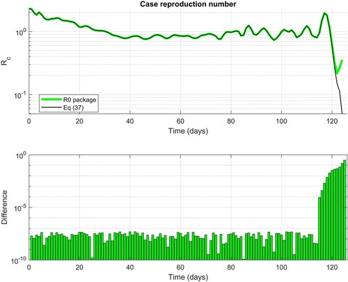
In Figure , we see that the calculation of by Equation (37) and those obtained by the R0 package using the Wallinga–Teunis method [Citation25] are practically identical; the absolute difference is less than
. The difference is noticeable towards the end of data; i.e. on the length of the vector giving the generation time. Calculation of
by formula (37) implicitly assumes that
; i.e.
for
. In particular, this yields
. The calculation of
that includes only valid data is therefore limited to
.
Figure 1. Comparison of the case reproduction number calculated by Equation (37) and R0 package using the Wallinga–Teunis method.
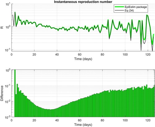
In Figure , we see that the absolute difference between the calculation of instantaneous reproduction number by Equation (34) and by function estimate_R from the EpiEstim package is in a range to
. The reason for the difference is that the function estimate_R implements a formula for calculating
, which, for statistical reasons, adds Gamma distribution parameters
in the numerator and
in the denominator of Equation (34) [Citation36]. We note that this has a side effect:
, even if
; however, it prevents the possibility of an undefined 0/0 case.
Figure 2. Comparison of the instantaneous reproduction number calculated by Equation (34) and by the function estimate_R from EpiEstim package.
Conclusion
We have shown that the well-known formulae for calculating the various epidemic reproduction numbers can be derived from the classical discrete Kermack–McKendrick epidemic model. An advantage of the model is that it is more intuitive and some of the assumptions of the continuous model can be omitted. In particular, as already mentioned, the derivation does not require a factorization assumption on the epidemic's transmissibility.
The practical example shows that case reproduction number calculated by the formula (37) gives numerically almost the same result as the reproduction number determined by the algorithmically much more demanding Wallinga–Teunis method.
Disclosure statement
No potential conflict of interest was reported by the author(s).
References
- N.P. Jewell, Statistics for Epidemiology, Chapman & Hall/CRC, Boca Raton, 2004.
- M. Woodward, Epidemiology Study Design and Data Analysis, CRC Press, Boca Raton, 2014.
- J.A.P. Heesterbeek, A brief history of R0 and a recipe for its calculation. Acta Biotheor. 50 (2002), pp. 189–204.
- J.M. Heffernan, R.J. Smith, and L.M. Wahl, Perspectives on the basic reproductive ratio. J. R Soc. Interface 2 (2005), pp. 281–293.
- R. Breban, R. Vardavas, and S. Blower, Theory versus data: how to calculate R0? Plos One 2 (2007), pp. 1–4.
- L.M.A. Bettencourt, and R.M. Ribeiro, Real time Bayesian estimation of the epidemic potential of Emerging infectious diseases. Plos One 3 (2008), pp. 1–9.
- B. Ridenhour, J.M. Kowalik, and D.K. Shay, Unraveling R0: considerations for public health applications. Am. J. Public Health 108 (2018), pp. S445–S454.
- P.L. Delamater, E.J. Street, T.F. Leslie, Y.T. Yang, and K.H. Jacobsen, Complexity of the basic reproduction number (R0). Emerg. Infect. Dis. 25 (2019), pp. 1–4.
- N.C. Grassly, and C. Fraser, Mathematical models of infectious disease transmission. Nat. Rev. Microbiol. 6 (2008), pp. 477–487.
- K. Dietz, Transmission and contol of arbovirus diseases, in Proceedings of SIMS Conference on Epidemiology Alta - Ut., July 8–12, 1974, D. Ludwig, K.L. Cooke, eds., Society for industrial and applied mathematics, Philadelphia, 1975. pp. 104–121.
- H.W. Hethcote, The mathematics of infectious diseases. SIAM Rev. 42 (2000), pp. 599–653.
- O. Diekmann, J.A.P. Heesterbeek, and J.A.J. Metz, On the definition and the computation of the basic reproduction ratio R0 in models for infectious–diseases in heterogeneous populations. J. Math. Biol. 28 (1990), pp. 365–382.
- K. Dietz, The estimation of the basic reproduction number for infectious diseases. Stat. Methods Med. Res. 2 (1993), pp. 23–41.
- J.A.P. Heesterbeek, and K. Dietz, The concept of R0 in epidemic theory. Stat. Neerl. 50 (1996), pp. 89–110.
- P. van den Driessche, and J. Watmough, Reproduction numbers and sub–threshold endemic equilibria for compartmental models of disease transmission. Math. Biosci. 180 (2002), pp. 29–48.
- C.P. Farrington, M.N. Kanaan, and N.J. Gay, Estimation of the basic reproduction number for infectious diseases from age–stratified serological survey data. J R Stat Soc C–Appl 50 (2001), pp. 251–283.
- M.G. Roberts, and J.A.P. Heesterbeek, Model–consistent estimation of the basic reproduction number from the incidence of an emerging infection. J. Math. Biol. 55 (2007), pp. 803–816.
- H. Nishiura, Correcting the actual reproduction number: A simple method to estimate R0 from early epidemic growth data. Int J Env Res Pub He 7 (2010), pp. 291–302.
- J.L. Ma, Estimating epidemic exponential growth rate and basic reproduction number. Infect Dis Model 5 (2020), pp. 129–141.
- L. Pellis, F. Ball, and P. Trapman, Reproduction numbers for epidemic models with households and other social structures. I. definition and calculation of R0. Math. Biosci. 235 (2012), pp. 85–97.
- P. van den Driessche, Reproduction numbers of infectious disease models. Infect Dis Model 2 (2017), pp. 288–303.
- G. Chowell, and F. Brauer, The basic reproduction number of infectious diseases: Computation and estimation Using compartmental epidemic models, in Mathematical and Statistical Estimation Approaches in Epidemiology, G. Chowell, J.M. Hyman, L.M.A. Bettencourt, C. Castillo–Chavez, ed., Springer, Dordrecht, 2009. pp. 363.
- P. Yan, Separate roles of the latent and infectious periods in shaping the relation between the basic reproduction number and the intrinsic growth rate of infectious disease outbreaks. J. Theor. Biol. 251 (2008), pp. 238–252.
- R. Ke, E. Romero-Severson, S. Sanche, and N. Hengartner, Estimating the reproductive number R0 of SARS–CoV–2 in the United States and eight european countries and implications for vaccination. J. Theor. Biol. 517 (2021), pp. 1–10.
- J. Wallinga, and P. Teunis, Different epidemic curves for severe acute respiratory syndrome reveal similar impacts of control measures, (2004).
- C. Fraser, Estimating individual and household reproduction numbers in an emerging epidemic. Plos One 2 (2007), pp. 1–12.
- L.F. White, and M. Pagano, A likelihood-based method for real-time estimation of the serial interval and reproductive number of an epidemic. Stat. Med. 27 (2008), pp. 2999–3016.
- G. Chowell, C. Viboud, L. Simonsen, and S.M. Moghadas, Characterizing the reproduction number of epidemics with early subexponential growth dynamics. J. R Soc. Interface 13 (2016), pp. 1–12.
- G. Chowell, and H. Nishiura, Quantifying the transmission potential of pandemic influenza. Phys. Life. Rev. 5 (2008), pp. 50–77.
- H. Nishiura, and G. Chowell, The effective reproduction number as a prelude to statistical estimation of time–dependent epidemic trends, in Mathematical and Statistical Estimation Approaches in Epidemiology, G. Chowell, J.M. Hyman, L.M.A. Bettencourt, C. Castillo–Chavez, ed., Springer, Dordrecht, 2009. pp. 103–122.
- J. Li, D. Blakeley, and R.J. Smith, The failure of R0. Comput Math Method M 2011 (2011), pp. 1–17.
- W.O. Kermack, and A.G. McKendrick, A contribution to the mathematical theory of epidemics, Proceedings of the Royal Society of London. Series A, Containing Papers of a Mathematical and Physical Character 115 (1927), pp. 700–721.
- A.G. McKendrick, Applications of mathematics to medical problems. Proceedings of the Edinburgh Mathematical Society 44 (1925), pp. 98–130.
- J. Wallinga, and M. Lipsitch, How generation intervals shape the relationship between growth rates and reproductive numbers. P Roy Soc B–Biol Sci 274 (2007), pp. 599–604.
- T. Obadia, R. Haneef, and P.Y. Boelle, The R0 package: a toolbox to estimate reproduction numbers for epidemic outbreaks. BMC Med Inform Decis 12 (2012), pp. 1–9.
- A. Cori, N.M. Ferguson, C. Fraser, and S. Cauchemez, A new framework and software to estimate time–varying reproduction numbers during epidemics. Am. J. Epidemiol. 178 (2013), pp. 1505–1512.
- R.N. Thompson, J.E. Stockwin, R.D. van Gaalen, J.A. Polonsky, Z.N. Kamvar, P.A. Demarsh, E. Dahlqwist, S. Li, E. Miguel, T. Jombart, J. Lessler, S. Cauchemez, and A. Cori, Improved inference of time–varying reproduction numbers during infectious disease outbreaks. Epidemics–Neth 29 (2019), pp. 1–11.
- F.Z. Brauer, and C. Castillo–Chávez, Discrete epidemic models. Math. Biosci. Eng. 7 (2010), pp. 1–15.
- O. Diekmann, and J.A.P. Heesterbeek, Mathematical Epidemiology of Infectious Diseases Model Building, Analysis and Interpretation, Wiley, Chichester, 2000.
- A. Svensson, A note on generation times in epidemic models. Math. Biosci. 208 (2007), pp. 300–311.
- S.W. Park, D. Champredon, J.S. Weitz, and J. Dushoff, A practical generation–interval–based approach to inferring the strength of epidemics from their speed. Epidemics–Neth 27 (2019), pp. 12–18.
- H. Nishiura, N.M. Linton, and A.R. Akhmetzhanov, Serial interval of novel coronavirus (COVID–19) infections. Int. J. Infect. Dis. 93 (2020), pp. 284–286.
- H. Nishiura, Time variations in the transmissibility of pandemic influenza in Prussia, Germany, from 1918–19. Theor. Biol. Med. Model. 4 (2007), pp. 1–9.
Appendix
MATLAB functions for calculation of the reproduction number.
function R0 = calcR0(w,r)
%CALCR0 Calculate basic reproduction number (Eq 29)
R0 = r/((exp(r) - 1)*sum(w.*exp(-r*(1:length(w)))));
end
function R = calcR(w,I)
%CALCR Calculate instantaneous reproduction number (Eq 34)
K = length(w);
N = length(I);
R = NaN(N,1);
for n = 1:N
s = 0;
for k = 1:min(n,K)
s = s + w(k)*I(n+1-k);
end
if s > 0
R(n) = I(n)/s;
end
end
end
function [Rc,R] = calcRc(w,I)
%CALCRC Calculate case reproduction number (Eq 37)
R = calcR(w,I);
K = length(w);
N = length(I);
Rc = NaN(N,1);
for n = 1:N
s = 0;
for k = 1:min(N-n+1,K)
s = s + w(k)*R(n+k-1);
end
Rc(n) = s;
end
end