Using an age-structured COVID-19 epidemic model and data to model virulence evolution in Wuhan, China

Abstract

COVID-19 is a disease caused by infection with the virus 2019-nCoV, a single-stranded RNA virus. During the infection and transmission processes, the virus evolves and mutates rapidly, though the disease has been quickly controlled in Wuhan by ‘Fangcang’ hospitals. To model the virulence evolution, in this paper, we formulate a new age structured epidemic model. Under the tradeoff hypothesis, two special scenarios are used to study the virulence evolution by theoretical analysis and numerical simulations. Results show that, before ‘Fangcang’ hospitals, two scenarios are both consistent with the data. After ‘Fangcang’ hospitals, Scenario I rather than Scenario II is consistent with the data. It is concluded that the transmission pattern of COVID-19 in Wuhan obey Scenario I rather than Scenario II. Theoretical analysis show that, in Scenario I, shortening the value of L (diagnosis period) can result in an enormous selective pressure on the evolution of 2019-nCoV.

Keywords:

• 2019-nCoV
• age structured model
• COVID-19
• virulence evolution
• ‘Fangcang’ hospitals

AMS Subject Classification(2010):

• 92B05

1. Introduction

Severe acute respiratory syndrome coronavirus 2 (2019-nCoV) is the causative agent of coronavirus disease (COVID-19). The virus emerged in Wuhan of China in December 2019 and quickly spread all over the world [1]. The World Health Organization declared the COVID-19 a pandemic on 11 March 2020 [1]. By end of June 2020, the virus has infected more than 10 million people worldwide and more than 500,000 of them have died [2]. In the process, it has forced massive lockdown and caused significant economic loss and devastation.

Because of its enormous public health impact and the need for guidance of health measures, many researchers have focused their efforts on the modelling of 2019-nCoV and its spread in the population (see mini review in [18]). Both mathematical models (e.g. [11,14]) and statistical approaches (e.g. [7]) have been used. The disease spread mechanism has been studied by using data fitting [9,11], and the disease spread has been forecasted in different regions to provide suggestions to government officials for the disease control, work resumption and return to school [3].

As of the end of June 2020, the spread of the disease in China has been contained. Medical technology and quarantine measures for the disease control are both improved significantly in mainland of China. Looking back at the course of the defense activities, quarantine policy played a key role. Especially, the quarantining of close contacts was very important. Following the progression of the disease, susceptible individuals who have been exposed undergo a short exposed period when they are not contagious. The exposed period lasts from exposure to 2 days before showing symptoms. After the exposed period, infected individuals become contagious, and after they show symptoms, they can be confirmed and possibly hospitalized [5].

While there are still many open questions on 2019-nCoV in regard to whether it imparts immunity and for how long, some very recent studies suggest that the virus is subject to continuous evolution [17]. By the tradeoff hypothesis, epidemic model with infection age has been used to study the virulence evolution. In the infection-age model, two scenarios, i.e. two pattern of transmission rate, were used to study the virulence evolution process [8].

On 12 February 2020, the government of Wuhan built several ‘Fangcang’ hospitals and more than 10,000 infected individuals were diagnosed and lived in a hospital. As a result, the spread of COVID-19 in Wuhan was quickly contained. Naturally, there are some questions that need to be addressed. Which is the key factor in the control of COVID-19 when 2019-nCoV continuously evolves? What is the virulence evolutionary path of 2019-nCoV?

To answer the above questions, the dynamic model should be involved in the distribution of quarantined individuals with respect to quarantined age ([4]) and the distribution of confirmed individuals with respect to confirmation age. Especially, the disease transmission process and the within host infection process should be linked by use of the infection age. Motivated by the above discussion, in this paper, we will formulate a new epidemic model involving infection age, confirmation age and quarantined age to study the virulence evolution of 2019-nCoV.

This paper is organized as follows. In Section 2, we establish a new age structured SEIJGR epidemic model to track the continuous infection stages, confirmation processes and quarantine period. Both theoretical and numerical analysis are carried out to reveal the virulence evolution of 2019-nCoV in two special scenarios in Section 3. Based on the data after 12 February 2020 and sensitivity analysis, our assessment works helps us identify the model of the virulence evolutionary path of 2019-nCoV in Section 4. In Section 5, we give a brief discussion.

2. Dynamical model of COVID-19 transmission

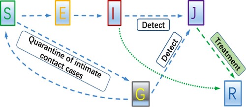
Motivated by the mechanism of COVID-19 transmission, we use the flowchart in Figure 1 to describe the disease spread and to formulate an SEIJGR epidemic model. In this model, $S\left(t\right)$ is the number of susceptible individuals at time t, $E\left(t\right)$ is the number of exposed individuals at time t who are not infectious; $I\left(t\right)$ is the number of infectious individuals at time t who have not been confirmed or detected, $J\left(t\right)$ is the total number of the confirmed and isolated individuals at time t and $G\left(t\right)$ is the total number of the quarantined individuals at time t. $R\left(t\right)$ is the total number of the recovered individuals at time t. Susceptible individuals get into a contact with an unconfirmed infective individual. A fraction $(1-\ell )$ of the newly infected individuals become exposed, while a fraction ℓ become quarantined. After the exposed period the undetected exposed individuals become undetected infectious and can be detected and isolated at rate ${\gamma }_1$.

Figure 1. Flow chart.

On 29th January, a paper in NEJM about 2019-nCoV spread in China [12] showed that the mean value of the time from infection to showing symptoms is 5.2 days $\in [4.1,7]$ (CI $95\mathrm{\%}$) and the maximum value is 12.5 days $\in [9,18]$ (CI $95\mathrm{\%}$). The same reference suggests that $89\mathrm{\%}$ of infectious individuals see a doctor more than 5 days since infected (see [12]). Thus symptoms appear on the average in the 6th day or later after exposure. Further, it is known that the exposed individuals may be infectious approximately 2 days before showing symptoms [5]. Hence, the exposed individuals cannot infect others in the first 4 days of infection [5]. Thus we assume that the transfer rate from the exposed to the infectious $\sigma =0.25$.

Note that the susceptible individuals will enter into the quarantined compartment at the ratio ℓ once they have been identified as close contacts of an infectious individual. The individuals in the quarantined compartment remain quarantined during the exposed period (5.2 days). Then the quarantined individuals either become confirmed and hospitalized or transfer into the susceptible class. We assume the recovery rate of quarantined individuals is ${\delta }_2=1/14$ [10,16] and the recovery rate of infected individuals in J class ${\delta }_1=0.1$ [15].

After 23 January 2020, when the lockdown of Wuhan started, the control measures started excerpting evolutionary pressure on the virus and the evolution of 2019-nCoV started play an important role in the disease transmission. To study the evolution of the virus, we will use two life histories of the virus which can be considered in the context of age-since-infection structured epidemic models [8]. Thus we address this disagreement by using an age-since-infection model:

(1) $\{\begin{array}{l}{\displaystyle \frac{\mathrm{d}S\left(t\right)}{\mathrm{d}t}=-S\left(t\right){\int }_0^{\mathrm{\infty }}\text{β}\left(a\right)I(a,t)\mathrm{d}a+{\delta }_2{\int }_0^{\mathrm{\infty }}G(\theta ,t)\mathrm{d}\theta ,}\\ {\displaystyle \frac{\mathrm{d}E\left(t\right)}{\mathrm{d}t}=(1-\ell )S\left(t\right){\int }_0^{\mathrm{\infty }}\text{β}\left(a\right)I(a,t)\mathrm{d}a-\sigma E\left(t\right),}\\ {\displaystyle \frac{\mathrm{\partial }I(a,t)}{\mathrm{\partial }a}+\frac{\mathrm{\partial }I(a,t)}{\mathrm{\partial }t}=-\left({\gamma }_1\right(a)+{\delta }_1)I(a,t),}\\ {\displaystyle I(0,t)=\sigma E\left(t\right),}\\ {\displaystyle \frac{\mathrm{\partial }J(b,t)}{\mathrm{\partial }b}+\frac{\mathrm{\partial }J(b,t)}{\mathrm{\partial }t}=-(\alpha +{\delta }_3(b\left)\right)J(b,t),}\\ {\displaystyle J(0,t)={\int }_0^{\mathrm{\infty }}{\gamma }_1\left(a\right)I(a,t)\mathrm{d}a+{\int }_0^{\mathrm{\infty }}{\gamma }_2\left(\theta \right)G(\theta ,t)\mathrm{d}\theta ,}\\ {\displaystyle \frac{\mathrm{\partial }G(\theta ,t)}{\mathrm{\partial }\theta }+\frac{\mathrm{\partial }G(\theta ,t)}{\mathrm{\partial }t}=-\left({\gamma }_2\right(\theta )+{\delta }_2)G(\theta ,t),}\\ {\displaystyle G(0,t)=\ell S\left(t\right){\int }_0^{\mathrm{\infty }}\text{β}\left(a\right)I(a,t)\mathrm{d}a,}\\ {\displaystyle \frac{\mathrm{d}R\left(t\right)}{\mathrm{d}t}={\delta }_1{\int }_0^{\mathrm{\infty }}I(a,t)\mathrm{d}a+{\int }_0^{\mathrm{\infty }}{\delta }_3\left(b\right)J(b,t)\mathrm{d}b,}\end{array}$(1)

with the initial conditions (2) $\{\begin{array}{l}{\displaystyle S\left(0\right)=S_0,E\left(0\right)=E_0,R\left(0\right)=R_0,}\\ {\displaystyle I(a,0)=I_0\left(a\right),J(a,0)=J_0\left(a\right),G(\theta ,0)=G_0\left(\theta \right).}\end{array}$(2) The independent variables a, b and θ in model (1(1) $\{\begin{array}{l}{\displaystyle \frac{\mathrm{d}S\left(t\right)}{\mathrm{d}t}=-S\left(t\right){\int }_0^{\mathrm{\infty }}\text{β}\left(a\right)I(a,t)\mathrm{d}a+{\delta }_2{\int }_0^{\mathrm{\infty }}G(\theta ,t)\mathrm{d}\theta ,}\\ {\displaystyle \frac{\mathrm{d}E\left(t\right)}{\mathrm{d}t}=(1-\ell )S\left(t\right){\int }_0^{\mathrm{\infty }}\text{β}\left(a\right)I(a,t)\mathrm{d}a-\sigma E\left(t\right),}\\ {\displaystyle \frac{\mathrm{\partial }I(a,t)}{\mathrm{\partial }a}+\frac{\mathrm{\partial }I(a,t)}{\mathrm{\partial }t}=-\left({\gamma }_1\right(a)+{\delta }_1)I(a,t),}\\ {\displaystyle I(0,t)=\sigma E\left(t\right),}\\ {\displaystyle \frac{\mathrm{\partial }J(b,t)}{\mathrm{\partial }b}+\frac{\mathrm{\partial }J(b,t)}{\mathrm{\partial }t}=-(\alpha +{\delta }_3(b\left)\right)J(b,t),}\\ {\displaystyle J(0,t)={\int }_0^{\mathrm{\infty }}{\gamma }_1\left(a\right)I(a,t)\mathrm{d}a+{\int }_0^{\mathrm{\infty }}{\gamma }_2\left(\theta \right)G(\theta ,t)\mathrm{d}\theta ,}\\ {\displaystyle \frac{\mathrm{\partial }G(\theta ,t)}{\mathrm{\partial }\theta }+\frac{\mathrm{\partial }G(\theta ,t)}{\mathrm{\partial }t}=-\left({\gamma }_2\right(\theta )+{\delta }_2)G(\theta ,t),}\\ {\displaystyle G(0,t)=\ell S\left(t\right){\int }_0^{\mathrm{\infty }}\text{β}\left(a\right)I(a,t)\mathrm{d}a,}\\ {\displaystyle \frac{\mathrm{d}R\left(t\right)}{\mathrm{d}t}={\delta }_1{\int }_0^{\mathrm{\infty }}I(a,t)\mathrm{d}a+{\int }_0^{\mathrm{\infty }}{\delta }_3\left(b\right)J(b,t)\mathrm{d}b,}\end{array}$(1) ) are the infection age (time since entering into the infectious class), the confirmation age (time since entering into the confirmed and isolated class) and the quarantine age (time since quarantined) respectively.

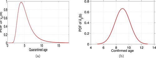
We surmise that the confirmation time of the quarantined individuals ${\gamma }_2\left(\theta \right)$ should obey a gamma distribution with the mean value 4 days, due to the mean value of the exposed period being 4 days ($\sigma =0.25$) and the exposed period ranging from 1 day to 14 days (see [4]). Further we assume that since the mean time of each confirmed individuals in hospital ${\delta }_3\left(b\right)$ is 9 days and the range is the interval [5, 12.75], the recovery time of the hospitalized obeys a normal distribution with minimum and the maximum recovery time of 5 days and 13 days and mean value of 9 days [6]. To summarize, we assume that the expressions for ${\gamma }_2\left(\theta \right)$ and ${\delta }_3\left(b\right)$ are gamma distribution function $28\times \mathrm{\Gamma }(32,8)$ and a normal distribution function $2.6\times \mathcal{N}(9,1.2)$ respectively (see Figure 2). The other parameters' values are given in Table 3.

Figure 2. The functions of ${\gamma }_2\left(\theta \right)$ and ${\delta }_2\left(b\right)$: (a) The function of ${\gamma }_2\left(\theta \right)$ and (b) the function of ${\delta }_2\left(b\right)$.

It follows from the idea of [13], we define the basic reproduction number of our model (1(1) $\{\begin{array}{l}{\displaystyle \frac{\mathrm{d}S\left(t\right)}{\mathrm{d}t}=-S\left(t\right){\int }_0^{\mathrm{\infty }}\text{β}\left(a\right)I(a,t)\mathrm{d}a+{\delta }_2{\int }_0^{\mathrm{\infty }}G(\theta ,t)\mathrm{d}\theta ,}\\ {\displaystyle \frac{\mathrm{d}E\left(t\right)}{\mathrm{d}t}=(1-\ell )S\left(t\right){\int }_0^{\mathrm{\infty }}\text{β}\left(a\right)I(a,t)\mathrm{d}a-\sigma E\left(t\right),}\\ {\displaystyle \frac{\mathrm{\partial }I(a,t)}{\mathrm{\partial }a}+\frac{\mathrm{\partial }I(a,t)}{\mathrm{\partial }t}=-\left({\gamma }_1\right(a)+{\delta }_1)I(a,t),}\\ {\displaystyle I(0,t)=\sigma E\left(t\right),}\\ {\displaystyle \frac{\mathrm{\partial }J(b,t)}{\mathrm{\partial }b}+\frac{\mathrm{\partial }J(b,t)}{\mathrm{\partial }t}=-(\alpha +{\delta }_3(b\left)\right)J(b,t),}\\ {\displaystyle J(0,t)={\int }_0^{\mathrm{\infty }}{\gamma }_1\left(a\right)I(a,t)\mathrm{d}a+{\int }_0^{\mathrm{\infty }}{\gamma }_2\left(\theta \right)G(\theta ,t)\mathrm{d}\theta ,}\\ {\displaystyle \frac{\mathrm{\partial }G(\theta ,t)}{\mathrm{\partial }\theta }+\frac{\mathrm{\partial }G(\theta ,t)}{\mathrm{\partial }t}=-\left({\gamma }_2\right(\theta )+{\delta }_2)G(\theta ,t),}\\ {\displaystyle G(0,t)=\ell S\left(t\right){\int }_0^{\mathrm{\infty }}\text{β}\left(a\right)I(a,t)\mathrm{d}a,}\\ {\displaystyle \frac{\mathrm{d}R\left(t\right)}{\mathrm{d}t}={\delta }_1{\int }_0^{\mathrm{\infty }}I(a,t)\mathrm{d}a+{\int }_0^{\mathrm{\infty }}{\delta }_3\left(b\right)J(b,t)\mathrm{d}b,}\end{array}$(1) ) as follows: (3) ${\mathcal{R}}_0=(1-\ell )S_0{\int }_0^{\mathrm{\infty }}\text{β}\left(a\right)e^{-{\int }_0^a\left({\gamma }_1\right(\tau )+{\delta }_1)\mathrm{d}\tau }\mathrm{d}a.$(3) In the next section, we use our model (1(1) $\{\begin{array}{l}{\displaystyle \frac{\mathrm{d}S\left(t\right)}{\mathrm{d}t}=-S\left(t\right){\int }_0^{\mathrm{\infty }}\text{β}\left(a\right)I(a,t)\mathrm{d}a+{\delta }_2{\int }_0^{\mathrm{\infty }}G(\theta ,t)\mathrm{d}\theta ,}\\ {\displaystyle \frac{\mathrm{d}E\left(t\right)}{\mathrm{d}t}=(1-\ell )S\left(t\right){\int }_0^{\mathrm{\infty }}\text{β}\left(a\right)I(a,t)\mathrm{d}a-\sigma E\left(t\right),}\\ {\displaystyle \frac{\mathrm{\partial }I(a,t)}{\mathrm{\partial }a}+\frac{\mathrm{\partial }I(a,t)}{\mathrm{\partial }t}=-\left({\gamma }_1\right(a)+{\delta }_1)I(a,t),}\\ {\displaystyle I(0,t)=\sigma E\left(t\right),}\\ {\displaystyle \frac{\mathrm{\partial }J(b,t)}{\mathrm{\partial }b}+\frac{\mathrm{\partial }J(b,t)}{\mathrm{\partial }t}=-(\alpha +{\delta }_3(b\left)\right)J(b,t),}\\ {\displaystyle J(0,t)={\int }_0^{\mathrm{\infty }}{\gamma }_1\left(a\right)I(a,t)\mathrm{d}a+{\int }_0^{\mathrm{\infty }}{\gamma }_2\left(\theta \right)G(\theta ,t)\mathrm{d}\theta ,}\\ {\displaystyle \frac{\mathrm{\partial }G(\theta ,t)}{\mathrm{\partial }\theta }+\frac{\mathrm{\partial }G(\theta ,t)}{\mathrm{\partial }t}=-\left({\gamma }_2\right(\theta )+{\delta }_2)G(\theta ,t),}\\ {\displaystyle G(0,t)=\ell S\left(t\right){\int }_0^{\mathrm{\infty }}\text{β}\left(a\right)I(a,t)\mathrm{d}a,}\\ {\displaystyle \frac{\mathrm{d}R\left(t\right)}{\mathrm{d}t}={\delta }_1{\int }_0^{\mathrm{\infty }}I(a,t)\mathrm{d}a+{\int }_0^{\mathrm{\infty }}{\delta }_3\left(b\right)J(b,t)\mathrm{d}b,}\end{array}$(1) ) and the cumulative confirmed case data in Wuhan before ‘Fangcang hospitals’ were introduced to perform data fitting. From the data fitting, we will obtain the values of the parameters related to the viral evolution, and then get a preliminary understanding on the evolution of 2019-nCoV.

3. Zooming in on the 2019-nCoV virulence evolution in conjunction with control measures

3.1. Fitting data to understand 2019-nCoV virulence evolution

In this section, we will carry out the data fitting to derive the values of the parameters $\text{β}\left(a\right)$ and ${\gamma }_1\left(a\right)$ which shed light on the viral evolution of its transmission rate $\text{β}\left(a\right)$ in terms of the control measures modelled by ${\gamma }_1\left(a\right)$. We also compute the value of the basic reproduction number ${\mathcal{R}}_0$ and obtain a rough understanding about the virulence evolution of 2019-nCov.

For the period starting on January 23, the initial conditions of our model are assumed as $S_0=6,081,000$, $E_0=750$ and $I_0\left(a\right),$ $J_0\left(b\right)$, $G_0\left(\theta \right)$ are given in Figure 3. The predetermined parameter values are given in Table 3. To carry out the data fitting, we will use the reported case data in Tables 1–2 and consider two highly simplified parasite life histories, captured through the form of the parameters $\text{β}\left(a\right)$ and ${\gamma }_1\left(a\right)$, which are taken as Scenario I and Scenario II from [8] (see Figure 4). These scenarios provide two possible virulence evolutionary paths of 2019-nCoV and help us get a clear understanding about the disease transmission mechanism.

Figure 3. Initial age distributions of $I_0\left(a\right)$, $J_0\left(b\right)$ and $G_0\left(\theta \right)$.

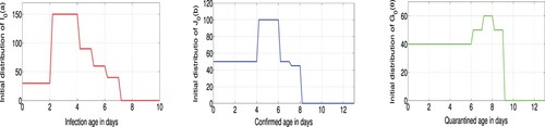
Figure 4. Two kinds of scenarios: (a) evolution function for scenario I and (b) evolution function for scenario II.

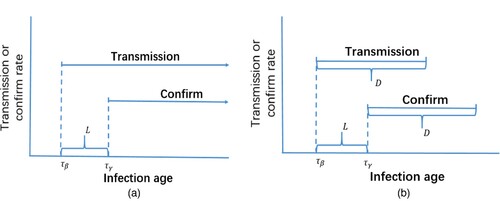
Table 1. Reported case data 23–31 January 2020, reported for Wuhan Municipality by the Wuhan Municipal Health Commission [19].

Data January	23	24	25	26	27	28	29	30	31
Confirmed cases (cumulative)	495	572	618	698	1590	1905	2261	2639	3215
Mortality cases (cumulative)	23	38	45	63	85	104	129	159	192

Table 2. Reported cumulative case data 1-11 February 2020, reported for Wuhan by the Wuhan Municipal Health Commission [19].

Feb	1	2	3	4	5	6	7	8	9	10	11
Com	4109	5142	6384	8351	10117	11618	13603	14982	16902	18454	19558
Mor	224	265	313	362	414	478	545	608	681	748	820

In Scenario I, we assume that transmission begins at infection age ${\tau }_{\text{β}}$ and is constant thereafter. Parasite-induced confirmation begins at infection age ${\tau }_{\gamma }$ and is constant thereafter. It then follows that (4) ${\gamma }_1\left(a\right)=\{\begin{array}{ll}{\gamma }_1,& a\ge {\tau }_{\gamma };\\ 0,& \text{otherwise}\end{array}\text{and}\text{β}\left(a\right)=\{\begin{array}{ll}\text{β},& a\ge {\tau }_{\text{β}};\\ 0,& \text{otherwise.}\end{array}$(4) Obviously, ${\tau }_{\gamma }$ is larger than ${\tau }_{\text{β}}$. Let $L={\tau }_{\gamma }-{\tau }_{\text{β}}$ (see Figure 4). Then the basic reproduction number simplifies to (5) ${\mathcal{R}}_0=(1-\ell )S_0{e}^{-{\delta }_1{\tau }_{\text{β}}}\text{β}(\frac{1-e^{-{\delta }_{1}L}}{{\delta }_1}+\frac{e^{-{\delta }_{1}L}}{{\gamma }_1+{\delta }_1}).$(5) In Scenario II, from Figure 4, we take (6) ${\gamma }_1\left(a\right)=\{\begin{array}{ll}{\gamma }_1,& {\tau }_{\gamma }\le a\le {\tau }_{\gamma }+D;\\ 0,& \text{otherwise}\end{array}\text{and}\text{β}\left(a\right)=\{\begin{array}{ll}\text{β},& {\tau }_{\text{β}}\le a\le {\tau }_{\text{β}}+D;\\ 0,& \text{otherwise.}\end{array}$(6) Obviously, ${\tau }_{\gamma }$ is larger than ${\tau }_{\text{β}}$, and we let $L<D<+\mathrm{\infty }$ (see Figure 4). Then it follows that the basic reproduction number takes the form (7) $\begin{array}{rl}{\mathcal{R}}_0{\displaystyle }& =(1-\ell )S_0{e}^{-{\delta }_1{\tau }_{\text{β}}}\text{β}[\frac{1-e^{-{\delta }_{1}L}}{{\delta }_1}+\frac{1-e^{-({\gamma }_1+{\delta }_1)(D-L)}}{{\gamma }_1+{\delta }_1}{e}^{-{\delta }_{1}L}]\\ & {\displaystyle =(1-\ell )S_0{e}^{-{\delta }_1{\tau }_{\gamma }}\text{β}[\frac{e^{{\delta }_{1}L}-1}{{\delta }_1}+\frac{1-e^{-({\gamma }_1+{\delta }_1)(D-L)}}{{\gamma }_1+{\delta }_1}].}\end{array}$(7) In the following, we will do data fitting based on our model (1(1) $\{\begin{array}{l}{\displaystyle \frac{\mathrm{d}S\left(t\right)}{\mathrm{d}t}=-S\left(t\right){\int }_0^{\mathrm{\infty }}\text{β}\left(a\right)I(a,t)\mathrm{d}a+{\delta }_2{\int }_0^{\mathrm{\infty }}G(\theta ,t)\mathrm{d}\theta ,}\\ {\displaystyle \frac{\mathrm{d}E\left(t\right)}{\mathrm{d}t}=(1-\ell )S\left(t\right){\int }_0^{\mathrm{\infty }}\text{β}\left(a\right)I(a,t)\mathrm{d}a-\sigma E\left(t\right),}\\ {\displaystyle \frac{\mathrm{\partial }I(a,t)}{\mathrm{\partial }a}+\frac{\mathrm{\partial }I(a,t)}{\mathrm{\partial }t}=-\left({\gamma }_1\right(a)+{\delta }_1)I(a,t),}\\ {\displaystyle I(0,t)=\sigma E\left(t\right),}\\ {\displaystyle \frac{\mathrm{\partial }J(b,t)}{\mathrm{\partial }b}+\frac{\mathrm{\partial }J(b,t)}{\mathrm{\partial }t}=-(\alpha +{\delta }_3(b\left)\right)J(b,t),}\\ {\displaystyle J(0,t)={\int }_0^{\mathrm{\infty }}{\gamma }_1\left(a\right)I(a,t)\mathrm{d}a+{\int }_0^{\mathrm{\infty }}{\gamma }_2\left(\theta \right)G(\theta ,t)\mathrm{d}\theta ,}\\ {\displaystyle \frac{\mathrm{\partial }G(\theta ,t)}{\mathrm{\partial }\theta }+\frac{\mathrm{\partial }G(\theta ,t)}{\mathrm{\partial }t}=-\left({\gamma }_2\right(\theta )+{\delta }_2)G(\theta ,t),}\\ {\displaystyle G(0,t)=\ell S\left(t\right){\int }_0^{\mathrm{\infty }}\text{β}\left(a\right)I(a,t)\mathrm{d}a,}\\ {\displaystyle \frac{\mathrm{d}R\left(t\right)}{\mathrm{d}t}={\delta }_1{\int }_0^{\mathrm{\infty }}I(a,t)\mathrm{d}a+{\int }_0^{\mathrm{\infty }}{\delta }_3\left(b\right)J(b,t)\mathrm{d}b,}\end{array}$(1) ) in Scenario I and Scenario II, respectively. By taking (8) ${\tau }_{\text{β}}=1\text{and}{\gamma }_1=0.4,$(8) we use the cumulative confirmed cases 23 January–11 February in Wuhan $Y_i$ to fit the variable $J_c$, which satisfies (9) $\frac{\mathrm{d}{J}_c\left(t\right)}{\mathrm{d}t}={\int }_0^{\mathrm{\infty }}{\gamma }_1\left(a\right)I(a,t)\mathrm{d}a+{\int }_0^{\mathrm{\infty }}{\gamma }_2\left(\theta \right)G(\theta ,t)\mathrm{d}\theta ,$(9) with the object function $min\sum _i(Y_i-J_c(t_i){)}^2.$ The values of the parameters β, L, ℓ and D are obtained in Table 4 and the fitting result is shown in Figure 5.

Figure 5. Data fitting results for the confirmed cases of 23 January–11 February Wuhan: (a) Scenario I and (b) Scenario II.

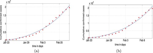
Table 3. Parameters of model (1(1) $\{\begin{array}{l}{\displaystyle \frac{\mathrm{d}S\left(t\right)}{\mathrm{d}t}=-S\left(t\right){\int }_0^{\mathrm{\infty }}\text{β}\left(a\right)I(a,t)\mathrm{d}a+{\delta }_2{\int }_0^{\mathrm{\infty }}G(\theta ,t)\mathrm{d}\theta ,}\\ {\displaystyle \frac{\mathrm{d}E\left(t\right)}{\mathrm{d}t}=(1-\ell )S\left(t\right){\int }_0^{\mathrm{\infty }}\text{β}\left(a\right)I(a,t)\mathrm{d}a-\sigma E\left(t\right),}\\ {\displaystyle \frac{\mathrm{\partial }I(a,t)}{\mathrm{\partial }a}+\frac{\mathrm{\partial }I(a,t)}{\mathrm{\partial }t}=-\left({\gamma }_1\right(a)+{\delta }_1)I(a,t),}\\ {\displaystyle I(0,t)=\sigma E\left(t\right),}\\ {\displaystyle \frac{\mathrm{\partial }J(b,t)}{\mathrm{\partial }b}+\frac{\mathrm{\partial }J(b,t)}{\mathrm{\partial }t}=-(\alpha +{\delta }_3(b\left)\right)J(b,t),}\\ {\displaystyle J(0,t)={\int }_0^{\mathrm{\infty }}{\gamma }_1\left(a\right)I(a,t)\mathrm{d}a+{\int }_0^{\mathrm{\infty }}{\gamma }_2\left(\theta \right)G(\theta ,t)\mathrm{d}\theta ,}\\ {\displaystyle \frac{\mathrm{\partial }G(\theta ,t)}{\mathrm{\partial }\theta }+\frac{\mathrm{\partial }G(\theta ,t)}{\mathrm{\partial }t}=-\left({\gamma }_2\right(\theta )+{\delta }_2)G(\theta ,t),}\\ {\displaystyle G(0,t)=\ell S\left(t\right){\int }_0^{\mathrm{\infty }}\text{β}\left(a\right)I(a,t)\mathrm{d}a,}\\ {\displaystyle \frac{\mathrm{d}R\left(t\right)}{\mathrm{d}t}={\delta }_1{\int }_0^{\mathrm{\infty }}I(a,t)\mathrm{d}a+{\int }_0^{\mathrm{\infty }}{\delta }_3\left(b\right)J(b,t)\mathrm{d}b,}\end{array}$(1) ).

Parameter	Interpretation	Value	Source
${\gamma }_2\left(\theta \right)$	Confirmed diagnostic rate from the quarantined	$28\times \mathrm{\Gamma }(32,8)$	Resource
${\delta }_3\left(b\right)$	Recovery rate of confirmed individuals	$2.6\times \mathcal{N}(9,1.2)$	Resource
${\gamma }_1\left(a\right)$	Confirmed diagnostic rate from the infected	–	Assumed
$\text{β}\left(a\right)$	Infection rate	–	Fitting
ℓ	Quarantine ratio	–	Fitting
${\delta }_1$	Recovery rate of infected individuals	0.1	[15]
${\delta }_2$	Recovery rate of quarantined individuals	1/14	[10,16]
α	Disease-induced death rate	0.02	Assumed
σ	transfer rate from the exposed to the infectious	0.25	Assumed

Table 4. Fitting results of model (1(1) $\{\begin{array}{l}{\displaystyle \frac{\mathrm{d}S\left(t\right)}{\mathrm{d}t}=-S\left(t\right){\int }_0^{\mathrm{\infty }}\text{β}\left(a\right)I(a,t)\mathrm{d}a+{\delta }_2{\int }_0^{\mathrm{\infty }}G(\theta ,t)\mathrm{d}\theta ,}\\ {\displaystyle \frac{\mathrm{d}E\left(t\right)}{\mathrm{d}t}=(1-\ell )S\left(t\right){\int }_0^{\mathrm{\infty }}\text{β}\left(a\right)I(a,t)\mathrm{d}a-\sigma E\left(t\right),}\\ {\displaystyle \frac{\mathrm{\partial }I(a,t)}{\mathrm{\partial }a}+\frac{\mathrm{\partial }I(a,t)}{\mathrm{\partial }t}=-\left({\gamma }_1\right(a)+{\delta }_1)I(a,t),}\\ {\displaystyle I(0,t)=\sigma E\left(t\right),}\\ {\displaystyle \frac{\mathrm{\partial }J(b,t)}{\mathrm{\partial }b}+\frac{\mathrm{\partial }J(b,t)}{\mathrm{\partial }t}=-(\alpha +{\delta }_3(b\left)\right)J(b,t),}\\ {\displaystyle J(0,t)={\int }_0^{\mathrm{\infty }}{\gamma }_1\left(a\right)I(a,t)\mathrm{d}a+{\int }_0^{\mathrm{\infty }}{\gamma }_2\left(\theta \right)G(\theta ,t)\mathrm{d}\theta ,}\\ {\displaystyle \frac{\mathrm{\partial }G(\theta ,t)}{\mathrm{\partial }\theta }+\frac{\mathrm{\partial }G(\theta ,t)}{\mathrm{\partial }t}=-\left({\gamma }_2\right(\theta )+{\delta }_2)G(\theta ,t),}\\ {\displaystyle G(0,t)=\ell S\left(t\right){\int }_0^{\mathrm{\infty }}\text{β}\left(a\right)I(a,t)\mathrm{d}a,}\\ {\displaystyle \frac{\mathrm{d}R\left(t\right)}{\mathrm{d}t}={\delta }_1{\int }_0^{\mathrm{\infty }}I(a,t)\mathrm{d}a+{\int }_0^{\mathrm{\infty }}{\delta }_3\left(b\right)J(b,t)\mathrm{d}b,}\end{array}$(1) ) for the data 23 January–11 February of Wuhan.

Para.	β	L	ℓ	D	${\mathcal{R}}_0$
Scenario I	3.2295$\times {10}^{-7}$	1.6262	0.6574	–	1.9485
Scenario II	3.3168$\times {10}^{-7}$	1.4627	0.6487	7.5195	1.9266

Figure 5 shows the real data is well fitted by our model when ${\gamma }_1=0.4$. Note that the value of ${\gamma }_1$ is influenced by the virulence of the virus. To improve the data fitting and obtain a rough understanding of the viral evolution, we will choose various values of ${\gamma }_1$ and perform the fitting for each one of them.

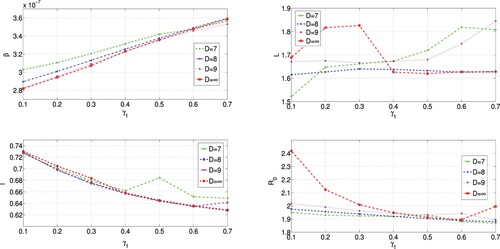
In Scenario I, we choose ${\gamma }_1=0.1$, 0.2, 0.3, 0.4, 0.5, 0.6, 0.7 respectively. From the results presented in Table 5, we see that the value of the transmission rate β is increasing with the increasing of the value of the confirmation rate ${\gamma }_1$. However, this dependence results in the decreasing of the value of the basic reproduction number ${\mathcal{R}}_0$, and the decreasing process seems to be steady. As we will see in the next section, analytical computations show that the increase of β with respect to ${\gamma }_1$ can be expected. This fact also demonstrates the accuracy of data fitting results. Even with the change, the values of β fall in the interval $[2.8202\times {10}^{-7},3.3168\times {10}^{-7}]$, and the value of ${\mathcal{R}}_0$ falls in an interval $[1.8967,2.4186]$.

Table 5. Fitting results of model (1(1) $\{\begin{array}{l}{\displaystyle \frac{\mathrm{d}S\left(t\right)}{\mathrm{d}t}=-S\left(t\right){\int }_0^{\mathrm{\infty }}\text{β}\left(a\right)I(a,t)\mathrm{d}a+{\delta }_2{\int }_0^{\mathrm{\infty }}G(\theta ,t)\mathrm{d}\theta ,}\\ {\displaystyle \frac{\mathrm{d}E\left(t\right)}{\mathrm{d}t}=(1-\ell )S\left(t\right){\int }_0^{\mathrm{\infty }}\text{β}\left(a\right)I(a,t)\mathrm{d}a-\sigma E\left(t\right),}\\ {\displaystyle \frac{\mathrm{\partial }I(a,t)}{\mathrm{\partial }a}+\frac{\mathrm{\partial }I(a,t)}{\mathrm{\partial }t}=-\left({\gamma }_1\right(a)+{\delta }_1)I(a,t),}\\ {\displaystyle I(0,t)=\sigma E\left(t\right),}\\ {\displaystyle \frac{\mathrm{\partial }J(b,t)}{\mathrm{\partial }b}+\frac{\mathrm{\partial }J(b,t)}{\mathrm{\partial }t}=-(\alpha +{\delta }_3(b\left)\right)J(b,t),}\\ {\displaystyle J(0,t)={\int }_0^{\mathrm{\infty }}{\gamma }_1\left(a\right)I(a,t)\mathrm{d}a+{\int }_0^{\mathrm{\infty }}{\gamma }_2\left(\theta \right)G(\theta ,t)\mathrm{d}\theta ,}\\ {\displaystyle \frac{\mathrm{\partial }G(\theta ,t)}{\mathrm{\partial }\theta }+\frac{\mathrm{\partial }G(\theta ,t)}{\mathrm{\partial }t}=-\left({\gamma }_2\right(\theta )+{\delta }_2)G(\theta ,t),}\\ {\displaystyle G(0,t)=\ell S\left(t\right){\int }_0^{\mathrm{\infty }}\text{β}\left(a\right)I(a,t)\mathrm{d}a,}\\ {\displaystyle \frac{\mathrm{d}R\left(t\right)}{\mathrm{d}t}={\delta }_1{\int }_0^{\mathrm{\infty }}I(a,t)\mathrm{d}a+{\int }_0^{\mathrm{\infty }}{\delta }_3\left(b\right)J(b,t)\mathrm{d}b,}\end{array}$(1) ) in Scenario I, 23 January–11 February.

Para. sequence	β	L	ℓ	${\mathcal{R}}_0$
${\gamma }_1=0.1$	2.8202$\times {10}^{-7}$	1.6889	0.7302	2.4186
${\gamma }_1=0.2$	2.9432$\times {10}^{-7}$	1.8167	0.7046	2.1244
${\gamma }_1=0.3$	3.0729$\times {10}^{-7}$	1.8260	0.6833	2.0090
${\gamma }_1=0.4$	3.2295$\times {10}^{-7}$	1.6262	0.6574	1.9485
${\gamma }_1=0.5$	3.3568$\times {10}^{-7}$	1.6200	0.6445	1.9127
${\gamma }_1=0.6$	3.4763$\times {10}^{-7}$	1.6274	0.6349	1.8967
${\gamma }_1=0.7$	3.5874$\times {10}^{-7}$	1.6284	0.6278	1.9959

In Scenario II, let ${\tau }_{\text{β}}=1$ and we take (10) $D=7\left(\text{days}\right),8\left(\text{days}\right),9\left(\text{days}\right),$(10) respectively. We perform again data fitting with values of ${\gamma }_1=0.1$, 0.15, 0.25, 0.3, 0.4, 0.5, 0.6, respectively for each fixed value of D. From the results presented in Tables 6–8, we see that the values of the transmission rate β are increasing with the increase of the values of the confirmation rate ${\gamma }_1$. A closer look at the results shows that the magnitudes of the increase of β are damping as the value of D decreases from 9 to 7. More specifically, the increase of the value of time lag L with respect to ${\gamma }_1$ is non-linear.

Table 6. Fitting results of model (1(1) $\{\begin{array}{l}{\displaystyle \frac{\mathrm{d}S\left(t\right)}{\mathrm{d}t}=-S\left(t\right){\int }_0^{\mathrm{\infty }}\text{β}\left(a\right)I(a,t)\mathrm{d}a+{\delta }_2{\int }_0^{\mathrm{\infty }}G(\theta ,t)\mathrm{d}\theta ,}\\ {\displaystyle \frac{\mathrm{d}E\left(t\right)}{\mathrm{d}t}=(1-\ell )S\left(t\right){\int }_0^{\mathrm{\infty }}\text{β}\left(a\right)I(a,t)\mathrm{d}a-\sigma E\left(t\right),}\\ {\displaystyle \frac{\mathrm{\partial }I(a,t)}{\mathrm{\partial }a}+\frac{\mathrm{\partial }I(a,t)}{\mathrm{\partial }t}=-\left({\gamma }_1\right(a)+{\delta }_1)I(a,t),}\\ {\displaystyle I(0,t)=\sigma E\left(t\right),}\\ {\displaystyle \frac{\mathrm{\partial }J(b,t)}{\mathrm{\partial }b}+\frac{\mathrm{\partial }J(b,t)}{\mathrm{\partial }t}=-(\alpha +{\delta }_3(b\left)\right)J(b,t),}\\ {\displaystyle J(0,t)={\int }_0^{\mathrm{\infty }}{\gamma }_1\left(a\right)I(a,t)\mathrm{d}a+{\int }_0^{\mathrm{\infty }}{\gamma }_2\left(\theta \right)G(\theta ,t)\mathrm{d}\theta ,}\\ {\displaystyle \frac{\mathrm{\partial }G(\theta ,t)}{\mathrm{\partial }\theta }+\frac{\mathrm{\partial }G(\theta ,t)}{\mathrm{\partial }t}=-\left({\gamma }_2\right(\theta )+{\delta }_2)G(\theta ,t),}\\ {\displaystyle G(0,t)=\ell S\left(t\right){\int }_0^{\mathrm{\infty }}\text{β}\left(a\right)I(a,t)\mathrm{d}a,}\\ {\displaystyle \frac{\mathrm{d}R\left(t\right)}{\mathrm{d}t}={\delta }_1{\int }_0^{\mathrm{\infty }}I(a,t)\mathrm{d}a+{\int }_0^{\mathrm{\infty }}{\delta }_3\left(b\right)J(b,t)\mathrm{d}b,}\end{array}$(1) ) in Scenario II, 23 January 23–11 February.

D = 7		Para. value
Para. sequence	β	L	ℓ	${\mathcal{R}}_0$
${\gamma }_1=0.1$	3.0278$\times {10}^{-7}$	1.5220	0.7259	1.9500
${\gamma }_1=0.2$	3.1053$\times {10}^{-7}$	1.6473	0.7010	1.9303
${\gamma }_1=0.3$	3.2063$\times {10}^{-7}$	1.6614	0.6790	1.9242
${\gamma }_1=0.4$	3.3131$\times {10}^{-7}$	1.6737	0.6619	1.9199
${\gamma }_1=0.5$	3.4203$\times {10}^{-7}$	1.7196	0.6488	1.9327
${\gamma }_1=0.6$	3.4740$\times {10}^{-7}$	1.8188	0.6515	1.8801
${\gamma }_1=0.7$	3.5654$\times {10}^{-7}$	1.8078	0.6448	1.8680

Table 7. Fitting results of model (1(1) $\{\begin{array}{l}{\displaystyle \frac{\mathrm{d}S\left(t\right)}{\mathrm{d}t}=-S\left(t\right){\int }_0^{\mathrm{\infty }}\text{β}\left(a\right)I(a,t)\mathrm{d}a+{\delta }_2{\int }_0^{\mathrm{\infty }}G(\theta ,t)\mathrm{d}\theta ,}\\ {\displaystyle \frac{\mathrm{d}E\left(t\right)}{\mathrm{d}t}=(1-\ell )S\left(t\right){\int }_0^{\mathrm{\infty }}\text{β}\left(a\right)I(a,t)\mathrm{d}a-\sigma E\left(t\right),}\\ {\displaystyle \frac{\mathrm{\partial }I(a,t)}{\mathrm{\partial }a}+\frac{\mathrm{\partial }I(a,t)}{\mathrm{\partial }t}=-\left({\gamma }_1\right(a)+{\delta }_1)I(a,t),}\\ {\displaystyle I(0,t)=\sigma E\left(t\right),}\\ {\displaystyle \frac{\mathrm{\partial }J(b,t)}{\mathrm{\partial }b}+\frac{\mathrm{\partial }J(b,t)}{\mathrm{\partial }t}=-(\alpha +{\delta }_3(b\left)\right)J(b,t),}\\ {\displaystyle J(0,t)={\int }_0^{\mathrm{\infty }}{\gamma }_1\left(a\right)I(a,t)\mathrm{d}a+{\int }_0^{\mathrm{\infty }}{\gamma }_2\left(\theta \right)G(\theta ,t)\mathrm{d}\theta ,}\\ {\displaystyle \frac{\mathrm{\partial }G(\theta ,t)}{\mathrm{\partial }\theta }+\frac{\mathrm{\partial }G(\theta ,t)}{\mathrm{\partial }t}=-\left({\gamma }_2\right(\theta )+{\delta }_2)G(\theta ,t),}\\ {\displaystyle G(0,t)=\ell S\left(t\right){\int }_0^{\mathrm{\infty }}\text{β}\left(a\right)I(a,t)\mathrm{d}a,}\\ {\displaystyle \frac{\mathrm{d}R\left(t\right)}{\mathrm{d}t}={\delta }_1{\int }_0^{\mathrm{\infty }}I(a,t)\mathrm{d}a+{\int }_0^{\mathrm{\infty }}{\delta }_3\left(b\right)J(b,t)\mathrm{d}b,}\end{array}$(1) ) in Scenario II, 23 January–11 February.

D = 8		Para. value
Para. sequence	β	L	ℓ	${\mathcal{R}}_0$
${\gamma }_1=0.1$	2.8955$\times {10}^{-7}$	1.6154	0.7280	1.9758
${\gamma }_1=0.2$	3.0089$\times {10}^{-7}$	1.6269	0.6982	1.9565
${\gamma }_1=0.3$	3.1311$\times {10}^{-7}$	1.6399	0.6754	1.9392
${\gamma }_1=0.4$	3.2544$\times {10}^{-7}$	1.6375	0.6582	1.9205
${\gamma }_1=0.5$	3.3746$\times {10}^{-7}$	1.6325	0.6453	1.9039
${\gamma }_1=0.6$	3.4890$\times {10}^{-7}$	1.6259	0.6357	1.8888
${\gamma }_1=0.7$	3.5965$\times {10}^{-7}$	1.6274	0.6285	1.8803

Table 8. Fitting results of model (1(1) $\{\begin{array}{l}{\displaystyle \frac{\mathrm{d}S\left(t\right)}{\mathrm{d}t}=-S\left(t\right){\int }_0^{\mathrm{\infty }}\text{β}\left(a\right)I(a,t)\mathrm{d}a+{\delta }_2{\int }_0^{\mathrm{\infty }}G(\theta ,t)\mathrm{d}\theta ,}\\ {\displaystyle \frac{\mathrm{d}E\left(t\right)}{\mathrm{d}t}=(1-\ell )S\left(t\right){\int }_0^{\mathrm{\infty }}\text{β}\left(a\right)I(a,t)\mathrm{d}a-\sigma E\left(t\right),}\\ {\displaystyle \frac{\mathrm{\partial }I(a,t)}{\mathrm{\partial }a}+\frac{\mathrm{\partial }I(a,t)}{\mathrm{\partial }t}=-\left({\gamma }_1\right(a)+{\delta }_1)I(a,t),}\\ {\displaystyle I(0,t)=\sigma E\left(t\right),}\\ {\displaystyle \frac{\mathrm{\partial }J(b,t)}{\mathrm{\partial }b}+\frac{\mathrm{\partial }J(b,t)}{\mathrm{\partial }t}=-(\alpha +{\delta }_3(b\left)\right)J(b,t),}\\ {\displaystyle J(0,t)={\int }_0^{\mathrm{\infty }}{\gamma }_1\left(a\right)I(a,t)\mathrm{d}a+{\int }_0^{\mathrm{\infty }}{\gamma }_2\left(\theta \right)G(\theta ,t)\mathrm{d}\theta ,}\\ {\displaystyle \frac{\mathrm{\partial }G(\theta ,t)}{\mathrm{\partial }\theta }+\frac{\mathrm{\partial }G(\theta ,t)}{\mathrm{\partial }t}=-\left({\gamma }_2\right(\theta )+{\delta }_2)G(\theta ,t),}\\ {\displaystyle G(0,t)=\ell S\left(t\right){\int }_0^{\mathrm{\infty }}\text{β}\left(a\right)I(a,t)\mathrm{d}a,}\\ {\displaystyle \frac{\mathrm{d}R\left(t\right)}{\mathrm{d}t}={\delta }_1{\int }_0^{\mathrm{\infty }}I(a,t)\mathrm{d}a+{\int }_0^{\mathrm{\infty }}{\delta }_3\left(b\right)J(b,t)\mathrm{d}b,}\end{array}$(1) ) in Scenario II, 23 January–11 February.

D = 9		Para. value
Para. sequence	β	L	ℓ	${\mathcal{R}}_0$
${\gamma }_1=0.1$	2.8219$\times {10}^{-7}$	1.6710	0.7289	2.0174
${\gamma }_1=0.2$	2.9556$\times {10}^{-7}$	1.6747	0.6976	1.9908
${\gamma }_1=0.3$	3.0928$\times {10}^{-7}$	1.6660	0.6741	1.9624
${\gamma }_1=0.4$	3.2271$\times {10}^{-7}$	1.6724	0.6567	1.9437
${\gamma }_1=0.5$	3.3552$\times {10}^{-7}$	1.6797	0.6440	1.9308
${\gamma }_1=0.6$	3.4573$\times {10}^{-7}$	1.7479	0.6347	1.9427
${\gamma }_1=0.7$	3.5300$\times {10}^{-7}$	1.8451	0.6418	1.8930

The results in Tables 6–8 show that the value of the basic reproduction number ${\mathcal{R}}_0$ is decreasing with the increase of the value of ${\gamma }_1$, and the monotonic decrease of ${\mathcal{R}}_0$ tends to stabilize. These data fitting results verify again the evolution of 2019-nCoV and show that the value of the basic reproduction number ${\mathcal{R}}_0$ falls in interval $[1.8680,1.9500]$, $[1.8803,1.9758]$, $[1.8903,2.0174]$ corresponding to D = 7, D = 8, D = 9, respectively.

Figure 6, corresponding to the results in Tables 5–8, has shown the relationships between different parameters. Figure 6(d) shows that the virus 2019-nCoV tries to keep the value of ${\mathcal{R}}_0$ as a constant which is larger than 1. Then the disease will persist if ${\mathcal{R}}_0>1$, based on the knowledge of infectious disease dynamics.

Figure 6. The evolution of β, L, ℓ and ${\mathcal{R}}_0$ as the value of ${\gamma }_1$ increases.

3.2. Understanding the virulence evolution of 2019-nCoV using theoretical results

In this section, we will justify the virulence evolution of 2019-nCoV results obtained from the fitting using analytical tools. It is assumed that the virulence evolution of 2019-nCoV is continuously and naturally before ‘Fangcang hospitals’, i.e. the case-confirmation rate ${\gamma }_1$ is totally determined by the virulence, the evolutionary path is fixed (one of the two scenarios).

Note that the disease transmission rate β and confirmation rate ${\gamma }_1$ are both derived from the virulence of 2019-nCoV. It is reasonable that the disease transmission rate β has a strong correlation with the confirmation rate ${\gamma }_1$ and the values of them are changing with the virulence evolution of 2019-nCoV. Based on the trade-off hypothesis [8], higher virulence is directly related to higher transmission which would help the virus spread, however, the higher virulence leads to higher confirmation rate which would reduce the virus spread. These results lead to the balance of disease transmission, and the magnitude of the basic reproduction number ${\mathcal{R}}_0$ will stay the same. Based on this idea, we will carry out the following theoretical analysis.

In Scenario I, ${\mathcal{R}}_0$ is given by Equation (5(5) ${\mathcal{R}}_0=(1-\ell )S_0{e}^{-{\delta }_1{\tau }_{\text{β}}}\text{β}(\frac{1-e^{-{\delta }_{1}L}}{{\delta }_1}+\frac{e^{-{\delta }_{1}L}}{{\gamma }_1+{\delta }_1}).$(5) ) and we treat β as a function of ${\gamma }_1$. Differentiating Equation (5(5) ${\mathcal{R}}_0=(1-\ell )S_0{e}^{-{\delta }_1{\tau }_{\text{β}}}\text{β}(\frac{1-e^{-{\delta }_{1}L}}{{\delta }_1}+\frac{e^{-{\delta }_{1}L}}{{\gamma }_1+{\delta }_1}).$(5) ) with respect to ${\gamma }_1$ and setting the derivative equal to zero, we obtain the following equation: (11) $\frac{{\text{β}}^{\prime }}{\text{β}}[(e^{{\delta }_{1}L}-1)\frac{{\gamma }_1+{\delta }_1}{{\delta }_1}+1]=\frac{1}{{\gamma }_1+{\delta }_1}.$(11) If L = 0, Equation (11(11) $\frac{{\text{β}}^{\prime }}{\text{β}}[(e^{{\delta }_{1}L}-1)\frac{{\gamma }_1+{\delta }_1}{{\delta }_1}+1]=\frac{1}{{\gamma }_1+{\delta }_1}.$(11) ) reduces to $\frac{{\text{β}}^{\prime }}{\text{β}}=\frac{1}{{\gamma }_1+{\delta }_1}$. Then β can be expressed as a function of ${\gamma }_1$, $\text{β}\left({\gamma }_1\right)=\text{β}\left(0\right)\frac{{\gamma }_1+{\delta }_1}{{\delta }_1}$, and it is an increasing function of the case-confirmation rate. If L>0, we get a simple interpretation of the time lag L from the left-hand side of Equation (11(11) $\frac{{\text{β}}^{\prime }}{\text{β}}[(e^{{\delta }_{1}L}-1)\frac{{\gamma }_1+{\delta }_1}{{\delta }_1}+1]=\frac{1}{{\gamma }_1+{\delta }_1}.$(11) ). The value of the factor in the square bracket is larger than one if L>0, and the growth rate of β with respect to ${\gamma }_1$ is smaller than that with L = 0. In the following, we will perform analysis to obtain a deeper understanding of the role of L in the virus's evolution processes. Let (12) $k=\frac{e^{{\delta }_{1}L}-1}{{\delta }_1}.$(12) Then, from (11(11) $\frac{{\text{β}}^{\prime }}{\text{β}}[(e^{{\delta }_{1}L}-1)\frac{{\gamma }_1+{\delta }_1}{{\delta }_1}+1]=\frac{1}{{\gamma }_1+{\delta }_1}.$(11) ), we have (13) $\frac{{\text{β}}^{\prime }}{\text{β}}=\frac{1}{\left(k\right({\gamma }_1+{\delta }_1)+1)({\gamma }_1+{\delta }_1)}=\frac{1}{{\gamma }_1+{\delta }_1}-\frac{k}{k({\gamma }_1+{\delta }_1)+1}.$(13) Integrating both sides of Equation (13(13) $\frac{{\text{β}}^{\prime }}{\text{β}}=\frac{1}{\left(k\right({\gamma }_1+{\delta }_1)+1)({\gamma }_1+{\delta }_1)}=\frac{1}{{\gamma }_1+{\delta }_1}-\frac{k}{k({\gamma }_1+{\delta }_1)+1}.$(13) ) with respect to ${\gamma }_1$ from 0 to ${\gamma }_1$, we have (14) $\text{β}\left({\gamma }_1\right)=\text{β}\left(0\right)\frac{{\gamma }_1+{\delta }_1}{{\delta }_1}\cdot \frac{k{\delta }_1+1}{(k{\delta }_1+1)+k{\gamma }_1}.$(14) Meanwhile, the factor $\frac{k{\delta }_1+1}{(k{\delta }_1+1)+k{\gamma }_1}\le 1,$ and it is decreasing with the increasing of k. Note that k is an increasing function of the time lag (diagnosis period) L (see (12(12) $k=\frac{e^{{\delta }_{1}L}-1}{{\delta }_1}.$(12) )). Thus the increasing of time lag L reduces the growth speed of β with respect to ${\gamma }_1$ and slows down the evolution speed of the virus. In the selective pressure the virulence is exerting on the transmission rate, the value of ${\gamma }_1$ is growing faster than the value of β as L increases. Therefore, shortening the value of L (diagnosis period) can result in an enormous selective pressure on the evolution of 2019-nCoV.

In Scenario II, treating β as a function of ${\gamma }_1$, we differentiate Equation (7(7) $\begin{array}{rl}{\mathcal{R}}_0{\displaystyle }& =(1-\ell )S_0{e}^{-{\delta }_1{\tau }_{\text{β}}}\text{β}[\frac{1-e^{-{\delta }_{1}L}}{{\delta }_1}+\frac{1-e^{-({\gamma }_1+{\delta }_1)(D-L)}}{{\gamma }_1+{\delta }_1}{e}^{-{\delta }_{1}L}]\\ & {\displaystyle =(1-\ell )S_0{e}^{-{\delta }_1{\tau }_{\gamma }}\text{β}[\frac{e^{{\delta }_{1}L}-1}{{\delta }_1}+\frac{1-e^{-({\gamma }_1+{\delta }_1)(D-L)}}{{\gamma }_1+{\delta }_1}].}\end{array}$(7) ) with respect to ${\gamma }_1$ and set it equal to zero and obtain the equation (15) $\frac{{\text{β}}^{\prime }}{\text{β}}[\frac{e^{{\delta }_{1}L}-1}{(1-e^{-({\gamma }_1+{\delta }_1)(D-L)})}\frac{{\gamma }_1+{\delta }_1}{{\delta }_1}+1]=\frac{1}{{\gamma }_1+{\delta }_1}-\frac{(D-L)e^{-({\gamma }_1+{\delta }_1)(D-L)}}{1-e^{-({\gamma }_1+{\delta }_1)(D-L)}}.$(15) Equation (15(15) $\frac{{\text{β}}^{\prime }}{\text{β}}[\frac{e^{{\delta }_{1}L}-1}{(1-e^{-({\gamma }_1+{\delta }_1)(D-L)})}\frac{{\gamma }_1+{\delta }_1}{{\delta }_1}+1]=\frac{1}{{\gamma }_1+{\delta }_1}-\frac{(D-L)e^{-({\gamma }_1+{\delta }_1)(D-L)}}{1-e^{-({\gamma }_1+{\delta }_1)(D-L)}}.$(15) ) will become Equation (11(11) $\frac{{\text{β}}^{\prime }}{\text{β}}[(e^{{\delta }_{1}L}-1)\frac{{\gamma }_1+{\delta }_1}{{\delta }_1}+1]=\frac{1}{{\gamma }_1+{\delta }_1}.$(11) ), when the value of D is infinity.

If the period D is finite, we can observe from Equation (15(15) $\frac{{\text{β}}^{\prime }}{\text{β}}[\frac{e^{{\delta }_{1}L}-1}{(1-e^{-({\gamma }_1+{\delta }_1)(D-L)})}\frac{{\gamma }_1+{\delta }_1}{{\delta }_1}+1]=\frac{1}{{\gamma }_1+{\delta }_1}-\frac{(D-L)e^{-({\gamma }_1+{\delta }_1)(D-L)}}{1-e^{-({\gamma }_1+{\delta }_1)(D-L)}}.$(15) ) that the growth of β with respect to ${\gamma }_1$ is nonlinear which agrees with the results in Tables 6–8 obtained from the fitting. However, comparing with the case when D is infinity, we conjecture that the finite period D slows down the evolution speed of the virus. Especially, the smaller the value of D, the smaller the dependence of β on ${\gamma }_1$ for $L<D<+\mathrm{\infty }$, which is consistent with data fitting results (see Figure 5).

From the above theoretical analysis, we get a main idea of the virulence evolution of 2019-nCoV from the perspective of the tradeoff hypothesis [8]. These theoretical results clearly show the relationship between ${\gamma }_1$ and β. It is reasonable to believe that β and ${\gamma }_1$ are positively coupled through their mutual dependence on host exploitation. Under the selective pressure, the virulence of 2019-nCoV forms a trade-off with transmission and confirmation, that is, the virulence chooses middle-of-the-virulence value to keep transmission and detection in balance and to coexist with humans for a long time. These two virulence evolutionary paths of 2019-nCoV (Scenario I and Scenario II) can provide reasonable explanations from theoretical analysis and data fitting. The problem which virulence evolutionary path is the true for 2019-nCoV is of interest. To investigate, we perform sensitivity analysis with the data after ‘Fangcang’ hospitals.

4. Sensitivity analysis

4.1. Determining key parameters of ${\mathcal{R}}_0$

 To understand better the virulence evolution of 2019-nCov, we perform sensitivity analysis of the basic reproduction number ${\mathcal{R}}_0$ in (5(5) ${\mathcal{R}}_0=(1-\ell )S_0{e}^{-{\delta }_1{\tau }_{\text{β}}}\text{β}(\frac{1-e^{-{\delta }_{1}L}}{{\delta }_1}+\frac{e^{-{\delta }_{1}L}}{{\gamma }_1+{\delta }_1}).$(5) ) (Scenario I) and (7(7) $\begin{array}{rl}{\mathcal{R}}_0{\displaystyle }& =(1-\ell )S_0{e}^{-{\delta }_1{\tau }_{\text{β}}}\text{β}[\frac{1-e^{-{\delta }_{1}L}}{{\delta }_1}+\frac{1-e^{-({\gamma }_1+{\delta }_1)(D-L)}}{{\gamma }_1+{\delta }_1}{e}^{-{\delta }_{1}L}]\\ & {\displaystyle =(1-\ell )S_0{e}^{-{\delta }_1{\tau }_{\gamma }}\text{β}[\frac{e^{{\delta }_{1}L}-1}{{\delta }_1}+\frac{1-e^{-({\gamma }_1+{\delta }_1)(D-L)}}{{\gamma }_1+{\delta }_1}].}\end{array}$(7) ) (Scenario II) with respect to its parameters. Based on the data fitting results, we employed Latin Hypercube Sampling (LHS) to identify the rank of key parameters that affect the basic reproduction number. Using the LHS technique with 100,000 samples, we plot the partial rank correlation coefficient (PRCC) respectively for Scenario I and Scenario II in Figure 7.

Figure 7. Partial rank correlation coefficients of ${\mathcal{R}}_0$ with respect to the parameters: (a) Scenario I and (b) Scenario II.

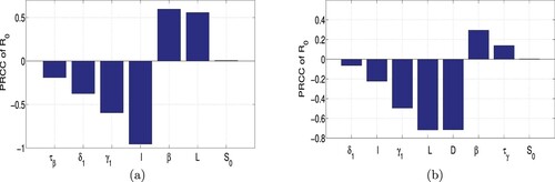
In Scenario I, from Figure 7 we see that the parameters ℓ, ${\gamma }_1$, β and L have PRCC larger than 0.5 in absolute value and are therefore the most sensitive parameters. Other parameters that are also influential are ${\delta }_1$ and ${\tau }_{\text{β}}$. Consequently improving the values of ℓ and ${\gamma }_1$ can lead to putting the disease under control. In Scenario II, we see that the parameters D, L, and ${\gamma }_1$ are the most sensitive parameters, and the parameters β, ℓ are no longer sensitive parameters. That raises the question whether improving the values of ${\gamma }_1$ and ℓ can lead to putting the disease under control. Note that D is the most influential parameter in Scenario II but it is not present in Scenario I. D will effect the multiples of the parameters ${\gamma }_1$ and ℓ.

These above differences between two evolutionary paths may give us a chance to investigate further the virulence evolutionary path of 2019-nCov by use of the data after ‘Fangcang’ hospitals.

4.2. Assessing control measures

The confirmation rate of COVID-19 is determined by the detection technology and the virulence of 2019-nCoV. Medical detection technology improves the value of ${\gamma }_1$, and epidemiological investigations increase the value of ℓ. ‘Fangcang’ hospitals provide sufficient space for the quarantined and confirmed individuals. Confirmation and quarantining were two useful and achievable interventions against the spread of COVID-19 in Wuhan. In this subsection, we will assess the role of these two control measures in the containment of COVID-19 in Wuhan.

In Scenario I, we obtained from the PRCC analysis that ℓ and ${\gamma }_1$ are the two most sensitive parameters. One important question is whether applying the control measures jointly is better than applying a single control measure. Another important question concerns the timing of control measures. Based on the evolution of 2019-nCoV, we will address the question of the timing of the intervention strategies.

If we use a single control strategy, namely detection of infected individuals, even if we increase the confirmation rate (replace the value of ${\gamma }_1$ by ${\gamma }_1=0.95$) and use the remaining parameters in lines 2, 4, 6 of Table 5, respectively (see Figure 8 (a)), we obtain that the theoretical plots of Figure 8 (a) are far away from the data. In another single control strategy, by increasing quarantining rate (replace the value of ℓ by $\ell =0.95$) from 12 February 2020 only, we perform simulations (see Figure 8 b), the theoretic plots also do not match the data. Results show that using a single measure is not enough.

Figure 8. Forecast without ‘Fangcang’ (left), with ‘Fangcang’ (right): (a) single control with ${\gamma }_1=0.2,0.4,0.6\to 0.95$ and (b) single control with $\ell \to 0.95$.

It is necessary to combine the two control measures. We need to both enhance the quarantine rate and improve the detection technology. By 11 February 2020, the detection technology was still relatively inadequate, and hence, the value of ${\gamma }_1$ is almost totally derived from the virulence of 2019-nCoV. After 11 February 2020, with the development of the nucleic acid detection, artificially improving the value of ${\gamma }_1$ became possible.

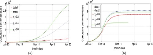
In Scenario I, the discussions in Section 3.2 show that the transmission rate β is monotonically increasing with respect to ${\gamma }_1$. The lower the value of ${\gamma }_1$ the smaller the value of β, and the more efficient the joint control measures. Numerical simulations show the effect of the control measures according to the real data (see Figure 9). In Scenario I, if the confirmation rate ${\gamma }_1$ is less than 0.2 before 11 February 2020, then the data of the cumulative confirmed cases will be matched by the joint control measures, otherwise, agreement between the data and the projections cannot be achieved. We conclude that the start of the joint control measures should occur when the disease transmission rate is very small (i.e. ${\gamma }_1=0.2$).

Figure 9. Simulation with improving ${\gamma }_1$ and ℓ at Feb. 12: (a) ${\gamma }_1$=0.2 $\to 0.55$ in Scenario I, (b) ${\gamma }_1$=0.1 $\to 0.95$, D = 7 in Scenario II, (c) ${\gamma }_1$=0.2 $\to 0.75$ in Scenario I, (d) ${\gamma }_1$=0.1 $\to 0.95$, D = 8 in Scenario II, (e) ${\gamma }_1$=0.2 $\to 0.95$ in Scenario I, (f) ${\gamma }_1$=0.1 $\to 0.95$, D = 9 in Scenario II.

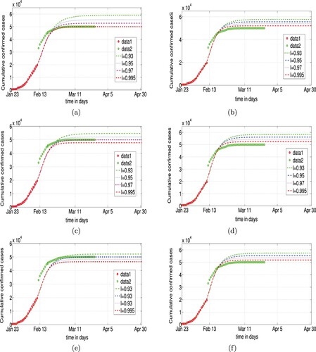
In Scenario II, the data of the cumulative confirmed cases cannot be matched by the joint control measures. Hence, we conclude that Scenario I is a better model of COVID-19 than Scenario II.

5. Discussion

It took 3 months to control COVID-19 in Wuhan, China, from the outbreak to the near elimination of the disease. Although it has been contained by the ‘Fangcang’ hospitals, a risk of a second outbreak still exists, potentially due to the virulence evolution of 2019-nCoV. In the context of infection age, confirmation age and quarantine age usually affect the viral evolution. In this paper, an age structured epidemic model is formulated to study the virulence evolution of 2019-nCoV by use of data and tradeoff hypothesis.

By taking two possible special scenarios as the virulence evolutionary paths of 2019-nCov, we perform data fitting based on our age structured epidemic model. Results show that the disease transmission rate and the confirmation rate of COVID-19 are strongly correlated before ‘Fanfcang’ hospitals. Using the tradeoff hypothesis in [8], we present theoretical analysis which deepens the understanding of the virulence evolution of 2019-nCov in two possible scenarios. In Scenario I, the virulence evolution of 2019-nCov is slowed down by the lag L which models the period of transmission before confirmation. In Scenario II, the transmission and confirmation only last for a fix duration D, and the value of D slows down the virulence evolution, compared with the virulence evolution in Scenario I.

Using sensitivity analysis, we find that the quarantining rate and the confirmation rate are two most sensitive parameters of the basic reproduction number in Scenario I, but they are not the most sensitive parameters in scenario II. Simulations suggest that after ‘Fangcang’ hospitals, the joint intervention measures play a key role in the disease control in both scenarios, regardless of the sensitivities of ℓ and ${\gamma }_1$. In Scenario I, the viral evolution process is simple and the COVID-19 can be controlled if the joint intervention measures be carried out as soon as possible. However, in Scenario II, the viral evolution process is complex, the control of COVID-19 spread will be more difficult.

Note that the disease is quickly controlled by ‘Fangcang’ hospitals in Wuhan. The assessment based on our age-structured SEIJGR epidemic model provides us an opportunity to identify the virulence evolutionary path of 2019-nCov. We find that Scenario I is a better model of virulence evolutionary path of 2019-nCov than Scenario II. Our theoretical analysis coupled with data gives us more clear understanding of 2019-nCoV and the disease COVID-19.

Acknowledgments

We would be very grateful to anonymous referees for their comments and suggestions that helped to improve this paper.

Disclosure statement

No potential conflict of interest was reported by the author(s).

Additional information

Funding

Supported partially by the National Natural Science Foundation of China [11771017, 12071293].

References

- Available at https://en.wikipedia.org/wiki/Severe_acute_respiratory_syndrome_coronavirus_2
- Available at https://www.worldometers.info/coronavirus/
- Available at https://www.cdc.gov/coronavirus/2019-nCoV/covid-data/mathematical-modeling.html
- Available at http://finance.sina.com.cn/stock/zqgd/2020-01-26/doc-iihnzhha4771155.shtml
- Available at https://www.webmd.com/lung/coronavirus-incubation-period
- Available at https://www.sohu.com/a/370590371_561670
- N. G. Davies, P. Klepac, Y. Liu, K. Prem, M. Jit, CMMID COVID-19 working group, and R. M. Eggo, Age-dependent effects in the transmission and control of COVID-19 epidemics, Nature Medicine. 26 (2020), pp. 1–7. doi: 10.1038/s41591-020-0962-9.
- T. Day, Virulence evolution and the timing of disease life-history events, TRENDS in Ecology and Evolution 18(3) (Mar 2003), pp. 113–118.
- G. Giordano, F. Blanchini, R. Bruno, P. Colaneri, A. Di Filippo, A. Di Matteo and M. Colaneri, Modelling the COVID-19 epidemic and implementation of population-wide interventions in Italy, Nature Medicine 26 (2020), pp. 855–860.
- Health Commission of Hubei Province, Available at http://wjw.hubei.gov.cn/bmdt/ztzl/fkxxgzbdgrfyyq/
- B. Ivorra, M. R. Ferrández, M. Vela-Pérez and A. M. Ramos, Mathematical modeling of the spread of the coronavirus disease 2019 (COVID-19) taking into account the undetected infections: the case of China, Commun Nonlinear Sci Numer Simul 88 (2020), pp. 105303.
- Q. Li, X. Guan, P. Wu, C. Wang, L. Zhou, Y. Tong, R. Ren, K. S. Leung, E. H. Lau, J. Y. Wong, and X. Xing, Early transmission dynamics in Wuhan, China, of novel Coronavirus-infected pneumonia, New England Journal of Medicine. doi: 10.1056/NEIMoa2001316.
- M. Martcheva, An Introduction to Mathematical Epidemiology, Springer, New York, 2015.
- F. Ndaïroua, I. Area, J. J. Nieto and D. F. M. Torres, Mathematical modeling of COVID-19 transmission dynamics with a case study of Wuhan, Chaos Solitons Fractals 135 (2020), pp. 109846.
- W. C. Roda, M. B. Varughese, D. Han and M. Y. Li, Why is it difficult to accurately predict the COVID-19 epidemic?, Infectious Disease Modelling 5 (2020), pp. 271–281.
- B. Tang, X. Wang, Q. Li, N. L. Bragazzi, S. Tang, Y. Xiao and J. Wu, Estimation of the transmission risk of 2019-nCov and its implication for public health interventions, Journal of Clinical Medicine 9 (2020), pp. 462.
- X. Tang, C. Wu, X. Li, Y. Song, X. Yao, X. Wu, Y. Duan, H. Zhang, Y. Wang, Z. Qian, J. Cui and J. Lu, On the origin and continuing evolution of SARS-CoV-2, National Science Review 7 (2020), pp. 1012–1023.
- N. Wang, Y. Fu, H. Zhang and H. Shi, An evaluation of mathematical models for the outbreak of COVID-19, Precision Clinical Medicine 3 (2020), pp. 85–93.
- Wuhan Municipal Health Commission, Available at http://wjw.wuhan.gov.cn/front/web/list3rd/yes/802