
 ?Mathematical formulae have been encoded as MathML and are displayed in this HTML version using MathJax in order to improve their display. Uncheck the box to turn MathJax off. This feature requires Javascript. Click on a formula to zoom.
Abstract
This paper is concerned with a modified Leslie–Gower and Holling-type II two-predator one-prey model with Lévy jumps. First, we use an Ornstein–Uhlenbeck process to describe the environmental stochasticity and prove that there is a unique positive solution to the system. Moreover, sufficient conditions for persistence in the mean and extinction of each species are established. Finally, we give some numerical simulations to support the main results.
1. Introduction
The relationship between prey and predator is one of the most important and interesting topics in biomathematics. Functional response is a significant component of the predator–prey relationship. The famous predator–prey framework with modified Leslie–Gower and Holling-type II schemes proposed by Aziz-Alaoui and Okiye [Citation4] can be denoted as follows:
(1)
(1) where
and
represent the population sizes of the prey and the predator, respectively.
and h are positive constants.
and
are the growth rates of the prey and the predator, respectively, a represents the competitive strength among individuals of the prey, c stands for the per capita reduction rate of prey x, the meaning of f is similar to c, and h describes the protection of the environment. Aziz-Alaoui and Okiye [Citation4] studied the boundedness and global stability of model (Equation1
(1)
(1) ). From then on, many authors have paid attention to model (Equation1
(1)
(1) ) and its generalized forms (see, e.g. [Citation1, Citation2, Citation5, Citation10–14, Citation26, Citation27, Citation30, Citation31, Citation33, Citation35]).
The above studies have focused on two-species models. However, it is a common phenomenon that several predators compete for a prey in the natural world. At the same time, the growth of the population is inevitably affected by environmental fluctuations in real situations. Suppose that the growth rate is affected by white noise (see, e.g. [Citation8, Citation15–17, Citation19, Citation24, Citation32, Citation37]), with
, Xu et al. [Citation32] proposed a stochastic two-predator one-prey system with modified Leslie–Gower and Holling-type II schemes:
where
is a standard Brownian motion defined on a complete probability space
with a filtration
satisfying the usual conditions and
stands for the intensity of the white noise.
However, the growth of species in the real world is often affected by sudden random perturbations, such as epidemics, harvesting, earthquakes, and so on; and these phenomena cannot be described by white noise. Bao and Yuan [Citation6] and Bao et al. [Citation7] suggested that these phenomena can be described by a Lévy jump process. Therefore, we can obtain the following two-predator one-prey model with white noise and Lévy jumps, which introduced Lévy noise into the population model in the same way as [Citation22]:
(2)
(2) with initial data
,
and
, where
,
and
are the left limit of
,
and
respectively. N is a Poisson counting measure with characteristic measure η on a measurable subset
of
with
,
,
is bounded and continuous with respect to η, and is
-measurable, i = 1, 2, 3.
Model (Equation2(2)
(2) ) assumes that the growth rate is linearly dependent on the Gaussian white noise in the random environments
Integrating on the interval
, we can see that
Hence, the variance of the average per capita growth rate
over an interval of length T tends to ∞ as
. According to this point, we can see that model (Equation2
(2)
(2) ) cannot accurately describe the real situation. Therefore, many authors (see [Citation9, Citation34]) have proposed that using the mean-reverting Ornstein–Uhlenbeck process is a more appropriate way to incorporate the environmental perturbations. On account of this approach, one has
i.e.
where
,
means the intensity of stochastic perturbations and
characterizes the speed of reversion. As a result, Zhou et al. [Citation36] considered the following stochastic model:
(3)
(3) Motivated by these, according to model (Equation2
(2)
(2) ), we can derive the following stochastic two-predator one-prey model with modified Leslie–Gower and Holling-type II schemes with Lévy jumps:
(4)
(4) To the best of our knowledge, there are few studies related to model (Equation4
(4)
(4) ), so we mainly study the properties of model (Equation4
(4)
(4) ) in this paper.
The rest of this paper is organized as follows. In Section 2, we give some lemmas for our main results and obtain sufficient conditions for persistence in the mean and extinction for each species. In Section 3, we introduce some simulation figures to illustrate our main theoretical results. Some concluding remarks are given in Section 4.
2. Main results
For convenience and simplicity, we define some notations as follows:
First, we give the following assumption and definition.
Assumption 2.1
There exists a constant m>0 such that
which means that the jump noise is not too strong.
Definition 2.1
[Citation22]
is said to be extinctive if
Before we state and prove our main results, we recall some lemmas which will be used later.
Lemma 2.1
[Citation23]
Suppose that , where
denotes the family of all positive-valued functions defined on
.
If there are three positive constants T,
If there are three positive constants T,
Lemma 2.2
[Citation20]
Suppose that , is a local martingale vanishing at time zero. Then
where
and
is Meyer's angle bracket process (see, e.g. [Citation3, Citation18]).
Lemma 2.3
For any given initial value , model (Equation4
(4)
(4) ) has a unique solution
for all
almost surely.
Proof.
To begin with, let us consider the following system:
(5)
(5) on
with initial data
,
,
. The coefficients of system (Equation5
(5)
(5) ) satisfy the local Lipschitz condition, then there is a unique local solution on
) (see Theorems 3.15–3.17 in [Citation25]), where
means the explosion time. Therefore, it follows from Itô's formula that on
) model (Equation4
(4)
(4) ) has a unique solution
which is positive. Now we validate
. Consider the following systems:
(6)
(6)
(7)
(7)
(8)
(8)
(9)
(9)
(10)
(10) On the basis of the comparison theorem [Citation28], we get for
),
(11)
(11) According to Lemma 4.2 in [Citation7], Equation (Equation6
(6)
(6) ) has the explicit formula
(12)
(12) Similarly
(13)
(13)
(14)
(14)
(15)
(15)
(16)
(16) Due to the fact that
,
,
,
, and
are existent on
, then we can obtain
.
Lemma 2.4
Let . If
(respectively,
), then
Proof.
Here we only prove the case , the proof of
is similar.
For sufficiently small , there is sufficiently large T such that, for
,
and for
,
Then when
, by (Equation12
(12)
(12) ),
where
Note that
. Consequently,
where
Moreover, for
, substituting the above inequalities into (Equation14
(14)
(14) ) leads to
where
For this reason,
(17)
(17) According to Assumption 2.1, we get
In view of Lemma 2.2, then
We then deduce from
that if
,
Substituting the above identities into (Equation17
(17)
(17) ) leads to
Now let us prove
Making use of Itô's formula to (Equation7
(7)
(7) ) deduces
That is to say
(18)
(18) For arbitrary given
, there exists T>0 such that, for
,
We then deduce from (Equation18
(18)
(18) ) that, for
,
(19)
(19)
(20)
(20) where ε is sufficiently small such that
. According to Lemma 2.1, we can obtain
We then deduce from the arbitrariness of ε that
which indicates that
In accordance with (Equation11
(11)
(11) ),
(21)
(21) The proof of Lemma 2.4 is completed.
Now we are in the position to give our main result.
Theorem 2.1
For model (Equation4(4)
(4) ), the following conclusions hold:
If
If
If
If
If
If
If
If
Proof.
(i). Taking advantage of Itô's formula to model (Equation4(4)
(4) ) gives
Integrating both sides from 0 to t, one can see that
(22)
(22)
(23)
(23)
(24)
(24) It follows from (Equation22
(22)
(22) ) that, for sufficiently large t,
(25)
(25) Note that
and
, then we have
In the same way, if
, it follows from (Equation23
(23)
(23) ) that
; if
, it follows from (Equation24
(24)
(24) ) that
(ii). Since , (i) implies
Then for sufficiently large t,
(26)
(26)
(27)
(27) Making use of Lemma 2.1 to (Equation26
(26)
(26) ) and (Equation27
(27)
(27) ), we can obtain that
According to the arbitrariness of ε, we have
The proof of (iii) and (iv) is similar to (ii), hence is omitted.
(v). Since , (i) implies
. Besides,
, for sufficiently large t, by (Equation22
(22)
(22) ), we obtain
(28)
(28)
(29)
(29) Making use of Lemma 2.1 to (Equation28
(28)
(28) ) and (Equation29
(29)
(29) ) results in
Making use of the arbitrariness of ε gives
(vi) Since , by (i) we know
.
(a) Computing yields
(30)
(30) On the basis of Lemma 2.4, for arbitrary
, there is a constant T>0 such that
, for
. For this reason,
for
. Substituting the above inequalities into (Equation30
(30)
(30) ) yields
(31)
(31) for all
almost surely. Let ε be sufficiently small such that
, thus
Then similar to the proof of (ii), we can prove
(b) By (Equation24
(24)
(24) ), we have
(32)
(32) We then deduce from Lemmas 2.2, 2.4 and
that
(33)
(33) As a result, for any
, we can find out T>0 such that, for
,
(34)
(34) Substituting (Equation34
(34)
(34) ) into (Equation22
(22)
(22) ), one can derive that
for sufficiently large t, where
obeys
. Then by Lemma 2.1,
Then the arbitrariness of ε means
The proof of (vii) is analogous to that of (vi) and hence is left out.
(viii) (e) Multiplying (Equation22(22)
(22) ), (Equation23
(23)
(23) ) and (Equation24
(24)
(24) ) by
,
and
, respectively, and then adding them, one gets that for sufficiently large t,
By virtue of Lemma 2.4, we can observe that for arbitrary
,
, and
As a result, for
,
(35)
(35) where ε satisfies
, thus
The proof of
is similar to (iv) and hence is omitted.
(f) Similar to the proof of (b) in (vi), we can get
Dividing both sides of (Equation22
(22)
(22) ) by t, we can get
(36)
(36) Choose
; on the basis of Lemma 2.1,
Using the arbitrariness of ε, one can observe that
This completes the proof.
3. Discussions and numerical simulations
Now we test the functions of the mean-reverting Ornstein–Uhlenbeck process on the persistence and extinction of Model (Equation4(4)
(4) ). We note that the speed of reversion
and the intensity of the perturbation
are two key parameters in the Ornstein–Uhlenbeck process. Theorem 2.1 shows that the persistence and extinction of system (Equation4
(4)
(4) ) are entirely dominated by the signs of
,
,
and
. Obviously,
Hence, as
(respectively,
) increases, species i tends to be persistent (respectively, extinct), i = 1, 2, 3. Moreover, due to the fact that
(respectively,
), so sufficiently large
(respectively,
) could make x extinct (respectively, persistent) if
and
. Similarly, sufficiently large
(respectively,
) could make x extinct (respectively, persistent) if
and
.
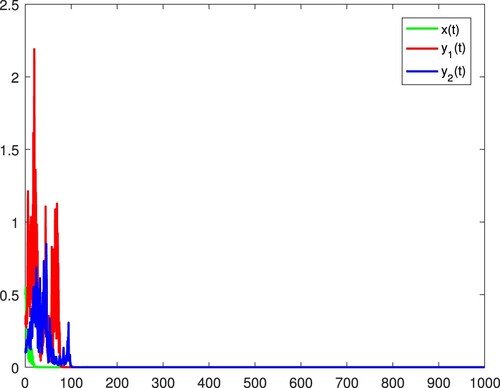
Now we use the Euler scheme offered in [Citation29] to prove our theoretical results numerically (here we only provide the functions of since the functions of
can be proffered analogously). Consider the following model:
(37)
(37) where
,
,
,
,
, and we suppose the initial data are
,
and
.
Choose
Choose
Choose
Choose
Choose
Comparing Figure with Figure , we can see that with the rise of
Choose
Choose
Comparing Figure with Figure , we can see that with the rise of
Choose
Choose
Comparing Figure with Figure , we can see that with the rise of
Choose
Choose
In Figure , we choose
Comparing Figure with Figure , we can see that with the rise of
In Figure , we choose
Comparing Figure with Figure , we can see that with the rise of
In Figure , we choose
Comparing Figure with Figure , we can see that with the rise of
Figure 1. All the species become extinct almost surely.
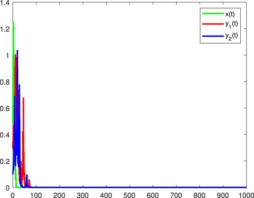
Figure 2. x and become extinct, and the species
is persistent in the mean almost surely.
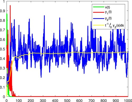
Figure 3. x and become extinct, and the species
is persistent in the mean almost surely.
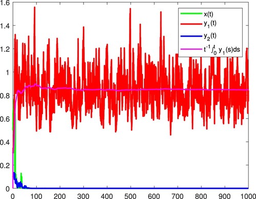
Figure 4. and
are persistent in the mean, and x becomes extinct almost surely.
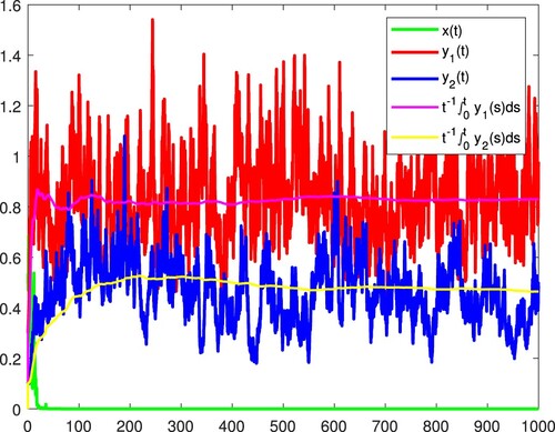
Figure 5. and
become extinct, and x is persistent in the mean almost surely.
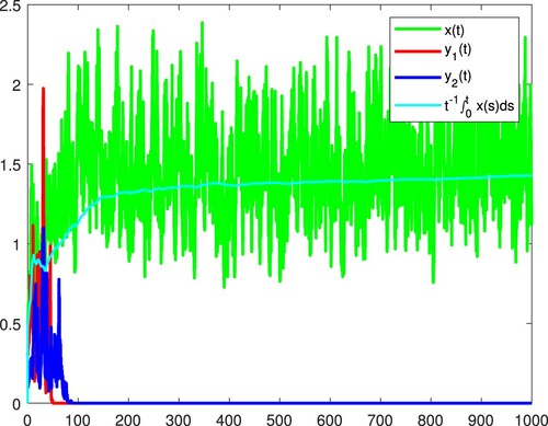
Figure 6. x and become extinct, and
is persistent in the mean almost surely.
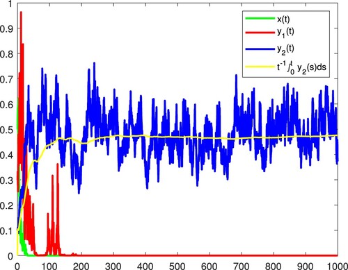
Figure 7. x and are persistent in the mean, and
becomes extinct almost surely.
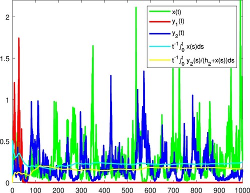
Figure 8. x and become extinct, and
is persistent in the mean almost surely.
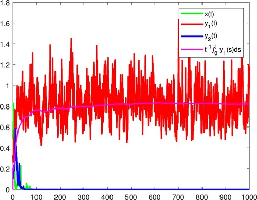
Figure 9. x and are persistent in the mean, and
becomes extinct almost surely.
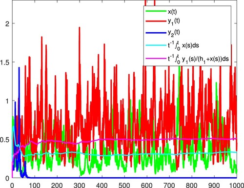
Figure 10. and
are persistent in the mean, and x becomes extinct almost surely.
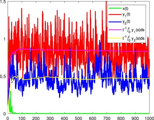
Figure 11. All the species are persistent in the mean almost surely.
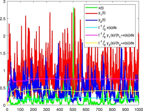
Figure 12. x and become extinct, and
is persistent in the mean almost surely.
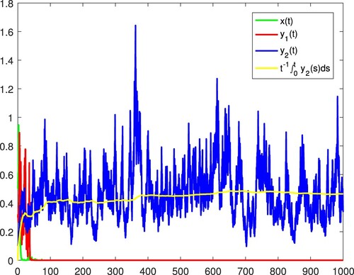
Figure 13. x and become extinct, and
is persistent in the mean almost surely.
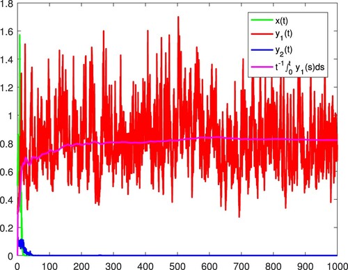
Figure 14. All the species are become extinct almost surely.
4. Concluding remarks
In this paper, we take advantage of a mean-reverting Ornstein–Uhlenbeck process to describe the random perturbations in the environment and formulate a stochastic three-species predator–prey system with Lévy jumps, which might be more appropriate to depict reality than model (Equation2(2)
(2) ). We obtain sharp sufficient conditions for persistence in the mean and extinction for each species of model (Equation4
(4)
(4) ) and uncovered some significant functions of Ornstein–Uhlenbeck process: sufficiently large
(the speed of reversion) could make species i persistent, i = 1, 2, 3; moreover, in some situations, sufficiently large
and
could make x become extinct.
Some interesting questions deserve further investigation. The present article probed into the white noises and Lévy noise, one could examine other random noises such as the telephone noise (see [Citation21]), etc. Besides, one could consider and investigate model (Equation4(4)
(4) ) in higher dimensions. All these considerations are left for future study.
Disclosure statement
No potential conflict of interest was reported by the author(s).
Additional information
Funding
References
- W. Abid, R. Yafia, M.A. Aziz-Alaoui, and A. Aghriche, Dynamics analysis and optimality in selective harvesting predator–prey model with modified Leslie–Gower and Holling-type II, Nonauton. Dyn. Syst. 6 (2019), pp. 1–17.
- N. Ali and M. Jazar, Global dynamics of a modified Leslie–Gower predator–prey model with Crowley–Martin functional responses, Appl. Math. Comput. 43 (2013), pp. 271–293.
- D. Applebaum, Lévy Processes and Stochastics Calculus, 2nd ed., Cambridge University Press, New York, 2009.
- M.A. Aziz-Alaoui and M.D. Okiye, Boundedness and global stability for a predator–prey model with modified Leslie–Gower and Holling-type II schemes, Appl. Math. Lett. 16 (2003), pp. 1069–1075.
- M. Banerjee and S. Banerjee, Turing instabilities and spatio-temporal chaos in ratio-dependent Holling–Tanner model, Math. Biosci. 236 (2012), pp. 64–76.
- J. Bao and C. Yuan, Stochastic population dynamics driven by Lévy noise, J. Math. Anal. Appl. 391 (2012), pp. 363–375.
- J. Bao, X. Mao, G. Yin, and C. Yuan, Competitive Lotka–Volterra population dynamics with jumps, Nonlinear Anal. 74 (2011), pp. 6601–6616.
- J.R. Beddington and R.M. May, Harvesting natural populations in a randomly fluctuating environment, Science 197 (1977), pp. 463–465.
- Y. Cai, J. Jiao, Z. Gui, Y. Liu, and W. Wang, Environmental variability in a stochastic epidemic model, Appl. Math. Comput. 329 (2018), pp. 210–226.
- J. Cao and R. Yuan, Bifurcation analysis in a modified Leslie–Gower model with Holling type II functional response and delay, Nonlinear Dyn. 84 (2016), pp. 1341–1352.
- F. Chen, L. Chen, and X. Xie, On a Leslie–Gower predator–prey model incorporating a prey refuge, Nonlinear Anal. Real World Appl. 10 (2009), pp. 2905–2908.
- R.K. Ghaziania, J. Alidousti, and A.B. Eshkaftaki, Stability and dynamics of a fractional order Leslie–Gower prey–predator model, Appl. Math. Model. 40 (2016), pp. 2075–2086.
- X. Guan, W. Wang, and Y. Cai, Spatiotemporal dynamics of a Leslie–Gower predator–prey model incorporating a prey refuge, Nonlinear Anal. Real World Appl. 12 (2011), pp. 2385–2395.
- H. Guo and X. Song, An impulsive predator–prey system with modified Leslie–Gower and Holling type II schemes, Chaos Solitons Fractals 36 (2008), pp. 1320–1331.
- C. Ji, D. Jiang, and N. Shi, Analysis of a predator–prey model with modified Leslie–Gower and Holling type II schemes with stochastic perturbation, J. Math. Anal. Appl. 359 (2009), pp. 482–498.
- C. Ji, D. Jiang, and N. Shi, A note on a predator–prey model with modified Leslie–Gower and Holling-type II schemes with stochastic perturbation, J. Math. Anal. Appl. 377 (2011), pp. 435–440.
- D. Jiang and N. Shi, A note on non-autonomous logistic equation with random perturbation, J. Math. Anal. Appl. 303 (2005), pp. 164–172.
- H. Kunita, Itô's stochastic calculus: its surprising power for applications, Stoch. Process. Appl. 120 (2010), pp. 622–652.
- X. Li and X. Mao, Population dynamical behavior of non-autonomous Lotka–Volterra competitive system with random perturbation, Discrete Contin. Dyn. Syst. 24 (2009), pp. 523–545.
- R.S. Lipster, A strong law of large numbers for local martingales, Stochastics 3 (1980), pp. 217–228.
- M. Liu, Dynamics of a stochastic regime-switching predator–prey model with modified Leslie–Gower Holling-type II schemes and prey harvesting, Nonlinear Dyn. 96 (2019), pp. 417–442.
- M. Liu and C. Bai, Dynamics of a stochastic one-prey two-predator model with Lévy jumps, Appl. Math. Comput. 284 (2016), pp. 308–321.
- M. Liu, K. Wang, and Q. Wu, Survival analysis of stochastic competitive models in a polluted environment and stochastic competitive exclusion principle, Bull. Math. Biol. 73 (2011), pp. 1969–2012.
- M. Liu, C. Du, and M. Deng, Persistence and extinction of a modified Leslie–Gower Holling-type II stochastic predator–prey model with impulsive toxicant input in polluted environments, Nonlinear Anal. Hybrid Syst. 27 (2018), pp. 177–190.
- X. Mao and C. Yuan, Stochastic Differential Equations with Markovian Switching, Imperial College Press, London, 2006
- L. Nie, Z. Teng, L. Hu, and J. Peng, Qualitative analysis of a modified Leslie–Gower and Holling-type II predator–prey model with state dependent impulsive effects, Nonlinear Anal. Real World Appl. 11 (2010), pp. 1364–1373.
- A.F. Nindjin, M.A. Aziz-Alaoui, and M. Cadivel, Analysis of a predator–prey model with modified Leslie–Gower and Holling-type II schemes with time delay, Nonlinear Anal. Real World Appl. 7 (2006), pp. 1104–1118.
- S. Peng and X. Zhu, Necessary and sufficient condition for comparison theorem of 1-dimensional stochastic differential equations, Stoch. Process. Appl. 116 (2006), pp. 370–380.
- P. Protter and D. Talay, The Euler scheme for Lévy driven stochastic differential equations, Ann. Probab. 25 (1997), pp. 393–423.
- X. Song and Y. Li, Dynamic behaviors of the periodic predator–prey model with modified Leslie–Gower Holling-type II schemes and impulsive effect, Nonlinear Anal. Real World Appl. 9 (2008), pp. 64–79.
- Y. Tian and P. Weng, Stability analysis of diffusive predator–prey model with modified Leslie–Gower and Holling-type III schemes, Appl. Math. Comput. 218 (2011), pp. 3733–3745.
- Y. Xu, M. Liu, and Y. Yang, Analysis of a stochastic two-predators one-prey system with modified Leslie–Gower and Holling-type II schemes, J. Appl. Anal. Comput. 7 (2017), pp. 713–727.
- R. Yafia, F. Adnani, and H. Alaoui, Limit cycle and numerical simulations for small and large delays in a predator–prey model with modified Leslie–Gower and Holling-type II schemes, Nonlinear Anal. Real World Appl. 9 (2008), pp. 2055–2067.
- Y. Zhao, S. Yuan, and J. Ma, Survival and stationary distribution analysis of a stochastic competitive model of three species in a polluted environment, Bull. Math. Biol. 77 (2015), pp. 1285–1326.
- J. Zhou, C. Kim, and J. Shi, Positive steady state solutions of a diffusive Leslie–Gower predator–prey model with Holling type II functional response and cross-diffusion, Discrete Contin. Dyn. Syst. 34 (2014), pp. 3875–3899.
- D. Zhou, M. Liu, and Z. Liu, Persistence and extinction of a stochastic predator–prey model with modified Leslie–Gower and Holling-type II schemes, Adv. Differ. Equ. 1 (2020), pp. 1–15.
- X. Zou, D. Fan, and K. Wang, Stationary distribution and stochastic Hopf bifurcation for a predator–prey system with noises, Discrete Contin. Dyn. Syst. Ser. B 18 (2013), pp. 1507–1519.