Dynamics analysis of stage-structured wild and sterile mosquito interaction impulsive model

Abstract

In this paper, we study a stage-structured wild and sterile mosquito interaction impulsive model. The aim is to study the feasibility of controlling the population of wild mosquitoes by releasing sterile mosquitoes periodically. The existence of trivial periodic solutions is obtained, and the corresponding local stability and global stability conditions are proved by Floquet theory and Lyapunov stability theorem, respectively. And we prove the existence conditions of non-trivial periodic solutions and their local stability. We can find that the system has the bistable phenomenon in which the trivial periodic solution and the non-trivial periodic solution can coexist under certain threshold conditions. All the results show that the appropriate release period and release amount of sterile mosquitoes can control the wild mosquito population within a certain range and even make them extinct. Finally, numerical simulation verifies our theoretical results.

Keywords:

• Stage-structure
• impulsive model
• periodic solutions
• bistability
• bifurcation

1. Introduction

Mosquito-borne diseases(MBDs) have been a serious health hazard in terms of human health. Dengue fever and a severe form of the disease described for the first time in the mid-1950, and it is estimated that up to 100 million cases of infection occur annually on a worldwide basis [25]. In mainland China, a number of dengue outbreaks have been reported since 1978, but the worst epidemic in decades, involving 45, 230 cases and 76 imported cases, resulting in 6 deaths in Guangdong province, emerged in 2014 [23]. Besides dengue fever, there are still several other MBDs that endanger human health, such as epidemic encephalitis B, malaria, filariasis, yellow fever, etc. Currently, the most effective method is to control the natural mosquito population [23].

In order to reduce the number of mosquitoes, people focus on using insecticides on a large scale. This method not only causes serious pollution to the environment but also makes mosquitoes resistant to drugs [32]. The Sterile Insect Technology (SIT) is a biological method widely applied to pest management around the world. The Cochliomyia hominivorax was driven out of Mexico [14]. The Bactrocera tryoni was controlled in South Australia [24]. The two sweetpotato pests, Cylas formicarius, and Euscepes postfasciatus were eradicated in Japan [26] and so on [10]. SIT still has good potential for controlling the size of the mosquito population.

The technology first irradiates mosquito pupae with a certain intensity of gamma rays. The irradiated mosquito pupae can mate with wild mosquitoes after hatching, but they do not lay eggs or eggs laid cannot hatch. Subsequently, these mosquitoes are repeatedly released into the environment in an overwhelming number. Sterile mosquitoes will greatly rob the wild mosquitoes from mating opportunities and thus achieve the purpose of controlling a large quantity of mosquitoes [5,9]. SIT succeeded in mosquito control practices and field experiments. From 2016 to 2017, the research team of Sun Yat-Sen University carried out open field trials. They used SIT in combination with Insect incompatibility Technology(IIT) on Aedes albopictus in the residential areas of two independent islands in Guangzhou, the main endemic area of dengue fever in China. It succeeded in reducing the number of mosquitoes by 83–94% per year [43]. The Brazilian scientific team succeeded in field tests of releasing sterile mosquitoes by using drones. From 2017 to 2018, up to 1 million mosquitoes were released a week over a period of 3 months at the peak of breeding, near the northeastern cities of Juazeiro and Recife [16].

Based on SIT, some biological mathematical methods, such as establishing and analysing mathematical models, are used to explain many hard problems of pest control. Since some years ago, quite a few ODE mathematical models have been formulated in [3–6,12] to study the interactive dynamics of the wild and sterile mosquito populations. In recent years, some more practical models have been proposed to test the feasibility of SIT in various environments [8,11,31,35–37,41,42,44]. For instance, models of unique and exact two periodic orbits, which consists of two sub-equations constantly switching each other [36,44], models of delay differential equation, which use the larvae maturation period of wild mosquitoes as time delay τ [35,37,41], a model of the predator–prey system with the monotone functional response, which incorporated the predation population as a distinct dynamical equation together with the wild and sterile insect pests [31].

Some studies usually assume that mosquito populations are homogeneous. Meanwhile, some studies have distinguished the stages of mosquito life. In reality, the life of a species often has a process of growth and development, and each stage of its growth will show unique characteristics. Mosquitoes are typically fully metamorphic insects, and the stage difference is particularly obvious. Mosquitoes need to go through four distinct stages of development during a lifetime: egg, larva, pupa, and adult [28]. There are significant differences in the physiological functions and living environment in each life stage, which largely affect their survival and extinction. In addition to predation and natural death, environmental crowding also has an important impact on mortality. Mosquitoes in the first three stages can only survive in the aquatic environment, but adult mosquitoes will fly away. The aquatic environment for mosquitoes is limited, especially in the range of human life, which leads to the crowding taking place in the first three aquatic stages of mosquito life. On the contrary, adult mosquitoes are hardly restricted by environmental capacity [13]. That is to say, the density-dependent mortality will occur in the first three stages of mosquito growth, but not in the adult stage. Therefore, in order to describe the dynamics of mosquito populations in line with the actual background, people introduce the stage-structure of mosquito growth into the population model.

Several researchers have been studied the stage-structured models [1,19,21,29,33,34,38, 40]. For instance, a model which distinguished the gender structure in the adult stage of mosquitoes was introduced in [38] and the dynamical analysis of the model revealed the existence of a forward bifurcation or a backward bifurcation with multiple attractors. Li et al. [21] established a population model of the interaction between wild and sterile mosquitoes with a stage-structure on the basis of ordinary differential equations. In [21,38,40], continuous systems were used to describe the dynamics of mosquito populations under different release methods. However, in [1,19,29,33,34], some discrete or semi-discrete models were used. In reality, for pest control practitioners, the periodic release of sterile mosquitoes may be more conducive to implementation. In this paper, based on the work in [21], we establish a semi-discrete model with stage-structure, and discuss the dynamics of the mosquito population under impulse control.

The article is arranged as follows. We first describe the establishment of the impulse model in Section 2. We then perform dynamic analysis on the model to obtain the existence and stability of the periodic solution in Section 3. Next, numerical simulation verifies our theoretical results in Section 4. We finally provide brief discussions of our findings in Section 5.

2. Model formulation

In the following, we introduce a mathematical model for the dynamics of mosquitoes, which was proposed and studied by Li et al. [21]. Then, on this basis, we propose an impulsive model, which is studied in this paper.

Firstly, we introduce the situation that a wild mosquito population without the presence of sterile mosquitoes. Mosquitoes show different characteristics at different stages. The first three aquatic stages of mosquitoes are classified as ‘Larvae’, denoted by J, and this part of mosquitoes will have density-dependent mortality due to the crowded aquatic environment. The mosquitoes in the latter stage are separately classified as ‘Adult’, denoted by A, and this part of mosquitoes will not be limited by environmental capacity, so they do not produce density-dependent mortality. In particular, the maturation rate for larvae was expressed as a function of the larvae population size rather than a fixed parameter, as in [20]. That is because the model assumed that there is a limit to the supply of living resources in water for larvae, which leads to a limit value $\alpha >0$ for the maturation rate of larvae. To describe such a limit, the maturation rate for larvae is represented as $\alpha (1-\kappa (J))$, which meets the following conditions: $0\le \kappa (J)\le 1$, with $\kappa (0)=0$, ${\kappa }^{\mathrm{\prime }}(J)>0$, and $\underset{J\to \mathrm{\infty }}{lim}\kappa (J)=1$. Based on such an idea, the following model was proposed in [21]. (1) $\{\begin{array}{rl}& {\displaystyle \frac{\mathrm{d}J}{\mathrm{d}t}}=\beta (\cdot )A-\alpha (1-\kappa (J))J-(d_0+d_{1}J)J,\\ & {\displaystyle \frac{\mathrm{d}A}{\mathrm{d}t}}=\alpha (1-\kappa (J))J-{\mu }_{1}A,\end{array}$(1) where $\beta (\cdot )$ is the oviposition rate of adults. The natural mortality rates of larvae and adult are denoted as $d_0$ and ${\mu }_1$, respectively. And the death rate due to density-dependent competition of the aquatic stage denoted by $d_{1}J$.

Further, same as [20], $\kappa (J)$ was taken as a functional response, that satisfies all of the assumptions, as (2) $\kappa (J)={\displaystyle \frac{J}{1+J}}.$(2) Thus system (1(1) $\{\begin{array}{rl}& {\displaystyle \frac{\mathrm{d}J}{\mathrm{d}t}}=\beta (\cdot )A-\alpha (1-\kappa (J))J-(d_0+d_{1}J)J,\\ & {\displaystyle \frac{\mathrm{d}A}{\mathrm{d}t}}=\alpha (1-\kappa (J))J-{\mu }_{1}A,\end{array}$(1) ) becomes (3) $\{\begin{array}{rl}& {\displaystyle \frac{\mathrm{d}J}{\mathrm{d}t}}=\beta (\cdot )A-{\displaystyle \frac{\alpha J}{1+J}}-(d_0+d_{1}J)J,\\ & {\displaystyle \frac{\mathrm{d}A}{\mathrm{d}t}}={\displaystyle \frac{\alpha J}{1+J}}-{\mu }_{1}A,\end{array}$(3) Then, we introduce the formula describing the release of sterile mosquitoes and let $g(t)$ be the number of sterile mosquitoes at time t. In order to explain the limitation of environmental capacity on mosquitoes, some models assume that sterile mosquitoes have a density-dependent mortality [36,37]. Meanwhile, in some models with age structures [1,19,21,29,33,34,38,40], sterile mosquitoes are usually regarded as not limited by environmental capacity and the limitation of environmental capacity exists only in the water in which the larvae live.

In this paper, we assume that adult mosquitoes and sterile mosquitoes have sufficient survival resources, thus sterile mosquitoes only have density-independent mortality, as in [1,19,21,29,33,34,38,40]. Since there is no natural reproduction for these mosquitoes, the birth rate for sterile mosquitoes is the rate of the releases. The dynamics of sterile mosquitoes are then determined by the following simple equation: (4) ${\displaystyle \frac{\mathrm{d}g}{\mathrm{d}t}}=B(\cdot )-{\mu }_{2}g,$(4) where $B(\cdot )$ is the sterile mosquito release rate, ${\mu }_2$ is the death rate of sterile mosquitoes. After the releasing of sterile mosquitoes, the interactive mating takes place. The birth function for the wild mosquitoes has the form (5) $\beta (\cdot )={\displaystyle \frac{\sigma A}{A+g}},$(5) where σ is the number of offspring produced per wild mosquito through all matings, per unit of time. Based on systems (3(3) $\{\begin{array}{rl}& {\displaystyle \frac{\mathrm{d}J}{\mathrm{d}t}}=\beta (\cdot )A-{\displaystyle \frac{\alpha J}{1+J}}-(d_0+d_{1}J)J,\\ & {\displaystyle \frac{\mathrm{d}A}{\mathrm{d}t}}={\displaystyle \frac{\alpha J}{1+J}}-{\mu }_{1}A,\end{array}$(3) ), (4(4) ${\displaystyle \frac{\mathrm{d}g}{\mathrm{d}t}}=B(\cdot )-{\mu }_{2}g,$(4) ) and (5(5) $\beta (\cdot )={\displaystyle \frac{\sigma A}{A+g}},$(5) ), the dynamics of the interactive wild and sterile mosquitoes are described by the following system [21]: (6) $\{\begin{array}{rl}& {\displaystyle \frac{\mathrm{d}J}{\mathrm{d}t}}={\displaystyle \frac{\sigma A}{A+g}}A-{\displaystyle \frac{\alpha J}{1+J}}-(d_0+d_{1}J)J,\\ & {\displaystyle \frac{\mathrm{d}A}{\mathrm{d}t}}={\displaystyle \frac{\alpha J}{1+J}}-{\mu }_{1}A,\\ & {\displaystyle \frac{\mathrm{d}g}{\mathrm{d}t}}=B(\cdot )-{\mu }_{2}g.\end{array}$(6) Most of the interaction models between wild and sterile mosquitoes are based on a continuous dynamic system. It means that a continuous release rate is usually used when describing the release process of sterile mosquitoes, and $B(\cdot )$ is a fixed constant. This is equivalent to assuming that the release of sterile mosquitoes is uninterrupted. However, in reality, the release process of mosquitoes is difficult to achieve continuously. The release of sterile mosquitoes is usually performed in multiples. For example, in 2017, Fresno County in the United States released 1 million sterile mosquitoes every week for 20 weeks [30]. From 2017 to 2018 Brazilian released 1 million mosquitoes a week over a period of 3 months, near the northeastern cities of Juazeiro and Recife [16]. Each release of sterile mosquitoes is manifested as an instantaneous change in the population, which will cause a pulse-like change in the population of sterile mosquitoes. Therefore, compared with the continuous system, the impulse system can describe the entire release process more reasonably. The impulse release model of sterile mosquitoes has received widespread attention [7,15,22,39]. Based on the above, we assume that the sterile mosquitoes are released every fixed time T, and the release amount is the same each time. The population dynamics of sterile mosquitoes can be expressed by impulsive differential equations (7) $\{\begin{array}{rl}& {\displaystyle \frac{\mathrm{d}g}{\mathrm{d}t}}=-{\mu }_{2}g,\\ & g(n{T}^{+})=g(nT)+b.\end{array}$(7) Based on systems (6(6) $\{\begin{array}{rl}& {\displaystyle \frac{\mathrm{d}J}{\mathrm{d}t}}={\displaystyle \frac{\sigma A}{A+g}}A-{\displaystyle \frac{\alpha J}{1+J}}-(d_0+d_{1}J)J,\\ & {\displaystyle \frac{\mathrm{d}A}{\mathrm{d}t}}={\displaystyle \frac{\alpha J}{1+J}}-{\mu }_{1}A,\\ & {\displaystyle \frac{\mathrm{d}g}{\mathrm{d}t}}=B(\cdot )-{\mu }_{2}g.\end{array}$(6) ) and (7(7) $\{\begin{array}{rl}& {\displaystyle \frac{\mathrm{d}g}{\mathrm{d}t}}=-{\mu }_{2}g,\\ & g(n{T}^{+})=g(nT)+b.\end{array}$(7) ), the dynamics of stage-structured wild and sterile mosquito interaction impulsive model are described by the following system: (8) $\{\begin{array}{rl}& {\displaystyle \frac{\mathrm{d}J}{\mathrm{d}t}}={\displaystyle \frac{\sigma A}{A+g}}A-{\displaystyle \frac{\alpha J}{1+J}}-(d_0+d_{1}J)J,\\ & {\displaystyle \frac{\mathrm{d}A}{\mathrm{d}t}}={\displaystyle \frac{\alpha J}{1+J}}-{\mu }_{1}A,\\ & {\displaystyle \frac{\mathrm{d}g}{\mathrm{d}t}}=-{\mu }_{2}g,\\ & g(n{T}^{+})=g(nT)+b,\end{array}$(8) where T is the release period, and b stands for a ‘per time’ number of sterile male mosquitoes to be released in the target locality.

3. Dynamics analysis

We shall present the Floquet theory for the impulsive equation [2].

Lemma 3.1

The impulsive equation (9) $\begin{array}{rl}& {\displaystyle \frac{\mathrm{d}x}{\mathrm{d}t}}=A(t)x,t\ne {\tau }_k,t\in R,\\ & \mathrm{\Delta }x=B_{k}x,t={\tau }_k,k\in z.\end{array}$(9) Introduce the following conditions (H3):

1. $A(\cdot )\in PC(R,C^{n\times n})$ and $A(t+T)=A(t)(t\in R)$.

2. $B_k\in C^{n\times n}$, $det(E+B_k)\ne 0$, ${\tau }_k<{\tau }_{k+1}(k\in Z)$.

3. There exists a $q\in N$ such that (10) $B_{k+q}=B_k,{\tau }_{k+q}={\tau }_k+T(k\in Z).$(10) Let conditions (H3) hold. Then each fundamental matrix of (9(9) $\begin{array}{rl}& {\displaystyle \frac{\mathrm{d}x}{\mathrm{d}t}}=A(t)x,t\ne {\tau }_k,t\in R,\\ & \mathrm{\Delta }x=B_{k}x,t={\tau }_k,k\in z.\end{array}$(9) ) can be represented in the form (11) $X(t)=\varphi (t)e^{\mathrm{\Lambda }t}(t\in R),$(11) where the matrix $\mathrm{\Lambda }\in C^{n\times n}$ is constant and the matrix $\varphi (\cdot )\in P{C}^1(R,C^{n\times n})$ is non-singular and T-periodic.

Lemma 3.2

Let conditions (H3) hold. Then the number $\omega \in C$ is a multiplier of (9(9) $\begin{array}{rl}& {\displaystyle \frac{\mathrm{d}x}{\mathrm{d}t}}=A(t)x,t\ne {\tau }_k,t\in R,\\ & \mathrm{\Delta }x=B_{k}x,t={\tau }_k,k\in z.\end{array}$(9) ) if and only if there exists a non-trivial solution $\phi (t)$ of (9(9) $\begin{array}{rl}& {\displaystyle \frac{\mathrm{d}x}{\mathrm{d}t}}=A(t)x,t\ne {\tau }_k,t\in R,\\ & \mathrm{\Delta }x=B_{k}x,t={\tau }_k,k\in z.\end{array}$(9) ) such that $\phi (t+T)=\omega \phi (t)(t\in R)$.

Lemma 3.3

Let conditions (H3) hold. Then the linear T-periodic impulsive Equation (9(9) $\begin{array}{rl}& {\displaystyle \frac{\mathrm{d}x}{\mathrm{d}t}}=A(t)x,t\ne {\tau }_k,t\in R,\\ & \mathrm{\Delta }x=B_{k}x,t={\tau }_k,k\in z.\end{array}$(9) ) is reducible to an equation with constant coefficients (12) ${\displaystyle \frac{\mathrm{d}y}{\mathrm{d}t}}=\mathrm{\Lambda }y,$(12) by a T-periodic Lyapunov transformation $x=\varphi (t)y$.

Lemma 3.4

Let conditions (H3) hold. Then the linear T-periodic impulsive Equation (9(9) $\begin{array}{rl}& {\displaystyle \frac{\mathrm{d}x}{\mathrm{d}t}}=A(t)x,t\ne {\tau }_k,t\in R,\\ & \mathrm{\Delta }x=B_{k}x,t={\tau }_k,k\in z.\end{array}$(9) ) is:

1. stable if and only if all multipliers ${\omega }_j(j=1,\dots ,n)$ of Equation (9(9) $\begin{array}{rl}& {\displaystyle \frac{\mathrm{d}x}{\mathrm{d}t}}=A(t)x,t\ne {\tau }_k,t\in R,\\ & \mathrm{\Delta }x=B_{k}x,t={\tau }_k,k\in z.\end{array}$(9) ) satisfy the inequality $\mid {\omega }_j\mid \le 1$ and, moreover, to those ${\omega }_j$ for which $\mid {\omega }_j\mid =1$ there correspond simple elementary divisors;

2. asymptotically stable if and only if all multipliers ${\omega }_j(j=1,\dots ,n)$ of Equation (9(9) $\begin{array}{rl}& {\displaystyle \frac{\mathrm{d}x}{\mathrm{d}t}}=A(t)x,t\ne {\tau }_k,t\in R,\\ & \mathrm{\Delta }x=B_{k}x,t={\tau }_k,k\in z.\end{array}$(9) ) satisfy the inequality $\mid {\omega }_j\mid <1$;

3. unstable if $\mid {\omega }_j\mid >1$ for some $j=1,\dots ,n$.

3.1. Trivial periodic solution and its stability

3.1.1. The existence of trivial periodic solution for system (8)

We first focus on the existence of trivial periodic solutions. The significance of the trivial periodic solution is that the mosquito population is extinct.

When $J(t)=0$, $A(t)=0$, then system (8(8) $\{\begin{array}{rl}& {\displaystyle \frac{\mathrm{d}J}{\mathrm{d}t}}={\displaystyle \frac{\sigma A}{A+g}}A-{\displaystyle \frac{\alpha J}{1+J}}-(d_0+d_{1}J)J,\\ & {\displaystyle \frac{\mathrm{d}A}{\mathrm{d}t}}={\displaystyle \frac{\alpha J}{1+J}}-{\mu }_{1}A,\\ & {\displaystyle \frac{\mathrm{d}g}{\mathrm{d}t}}=-{\mu }_{2}g,\\ & g(n{T}^{+})=g(nT)+b,\end{array}$(8) ) can be simplified to (13) $\{\begin{array}{rl}& {\displaystyle \frac{\mathrm{d}J}{\mathrm{d}t}}=0,\\ & {\displaystyle \frac{\mathrm{d}A}{\mathrm{d}t}}=0,\\ & {\displaystyle \frac{\mathrm{d}g}{\mathrm{d}t}}=-{\mu }_{2}g,\\ & g(n{T}^{+})=g(nT)+b.\end{array}$(13) From the last two equations of system (13(13) $\{\begin{array}{rl}& {\displaystyle \frac{\mathrm{d}J}{\mathrm{d}t}}=0,\\ & {\displaystyle \frac{\mathrm{d}A}{\mathrm{d}t}}=0,\\ & {\displaystyle \frac{\mathrm{d}g}{\mathrm{d}t}}=-{\mu }_{2}g,\\ & g(n{T}^{+})=g(nT)+b.\end{array}$(13) ) (14) $g[(n+1)T^{+}]=g(n{T}^{+})e^{-{\mu }_{2}T}+b,$(14) this discrete system satisfies when $n\to \mathrm{\infty }$, then (15) $g^{\ast }=\frac{b}{1-e^{-{\mu }_{2}T}}.$(15) Therefore, system (8(8) $\{\begin{array}{rl}& {\displaystyle \frac{\mathrm{d}J}{\mathrm{d}t}}={\displaystyle \frac{\sigma A}{A+g}}A-{\displaystyle \frac{\alpha J}{1+J}}-(d_0+d_{1}J)J,\\ & {\displaystyle \frac{\mathrm{d}A}{\mathrm{d}t}}={\displaystyle \frac{\alpha J}{1+J}}-{\mu }_{1}A,\\ & {\displaystyle \frac{\mathrm{d}g}{\mathrm{d}t}}=-{\mu }_{2}g,\\ & g(n{T}^{+})=g(nT)+b,\end{array}$(8) ) has a trivial periodic solution corresponding to the extinction of wild mosquitoes (16) $(\overline{J}(t),\overline{A}(t),\overline{g}(t))=(0,0,g^{\ast }{e}^{-{\mu }_2(tmodT)}).$(16)

3.1.2. The local stability of trivial periodic solutions for system (8)

Theorem 3.1

The trivial periodic solution $(\overline{J}(t),\overline{A}(t),\overline{g}(t))=(0,0,g^{\ast }{e}^{-{\mu }_2(tmodT)})$ of system (8(8) $\{\begin{array}{rl}& {\displaystyle \frac{\mathrm{d}J}{\mathrm{d}t}}={\displaystyle \frac{\sigma A}{A+g}}A-{\displaystyle \frac{\alpha J}{1+J}}-(d_0+d_{1}J)J,\\ & {\displaystyle \frac{\mathrm{d}A}{\mathrm{d}t}}={\displaystyle \frac{\alpha J}{1+J}}-{\mu }_{1}A,\\ & {\displaystyle \frac{\mathrm{d}g}{\mathrm{d}t}}=-{\mu }_{2}g,\\ & g(n{T}^{+})=g(nT)+b,\end{array}$(8) ) is always locally asymptotically stable.

Proof.

Define small amplitude perturbations of system (8(8) $\{\begin{array}{rl}& {\displaystyle \frac{\mathrm{d}J}{\mathrm{d}t}}={\displaystyle \frac{\sigma A}{A+g}}A-{\displaystyle \frac{\alpha J}{1+J}}-(d_0+d_{1}J)J,\\ & {\displaystyle \frac{\mathrm{d}A}{\mathrm{d}t}}={\displaystyle \frac{\alpha J}{1+J}}-{\mu }_{1}A,\\ & {\displaystyle \frac{\mathrm{d}g}{\mathrm{d}t}}=-{\mu }_{2}g,\\ & g(n{T}^{+})=g(nT)+b,\end{array}$(8) ) that $\tilde{J}=J-\overline{J}$, $\tilde{A}=A-\overline{A}$, $\tilde{g}=g-\overline{g}$. The impulse term disappears at this time (17) $\tilde{g}(n{T}^{+})=[g(nT)+b]-[\overline{g}(nT)+b]=\tilde{g}(nT).$(17) The system becomes (18) $\{\begin{array}{rl}{\displaystyle \frac{\mathrm{d}\tilde{J}}{\mathrm{d}t}}& ={\displaystyle \frac{\sigma \tilde{A}}{\tilde{A}+\tilde{g}+\overline{g}}}\tilde{A}-{\displaystyle \frac{\alpha \tilde{J}}{1+\tilde{J}}}-(d_0+d_1\tilde{J})\tilde{J},\\ {\displaystyle \frac{\mathrm{d}\tilde{A}}{\mathrm{d}t}}& ={\displaystyle \frac{\alpha \tilde{J}}{1+\tilde{J}}}-{\mu }_1\tilde{A},\\ {\displaystyle \frac{\mathrm{d}\tilde{g}}{\mathrm{d}t}}& =-{\mu }_2\tilde{g}.\end{array}$(18) Record it as (19) $\left(\begin{array}{c}\tilde{J}(t)\\ \tilde{A}(t)\\ \tilde{g}(t)\end{array}\right)=\mathrm{\Phi }(t)\left(\begin{array}{c}\tilde{J}(0)\\ \tilde{A}(0)\\ \tilde{g}(0)\end{array}\right),$(19) and the $\mathrm{\Phi }(t)$ satisfies (20) $\frac{\mathrm{d}\mathrm{\Phi }(t)}{\mathrm{d}t}=\mathrm{\Lambda }(t)\mathrm{\Phi }(t),$(20) where (21) $\mathrm{\Lambda }(t)=\left(\begin{array}{ccc}-{\displaystyle \frac{\alpha }{(1+\tilde{J}{)}^2}}-d_0-2d_1\tilde{J}& {\displaystyle \frac{\sigma \tilde{A}}{\tilde{A}+\tilde{g}+\overline{g}}}(1+{\displaystyle \frac{\tilde{g}+\overline{g}}{\tilde{A}+\tilde{g}+\overline{g}}})& -{\displaystyle \frac{\sigma {\tilde{A}}^2}{(\tilde{A}+\tilde{g}+\overline{g}{)}^2}}\\ {\displaystyle \frac{\alpha }{(1+\tilde{J}{)}^2}}& -{\mu }_1& 0\\ 0& 0& -{\mu }_2\end{array}\right).$(21) When $\tilde{A}(t)=0$, $\tilde{J}(t)=0$, then (22) $\mathrm{\Lambda }(t)=\left(\begin{array}{ccc}-\alpha -d_0& 0& 0\\ \alpha & -{\mu }_1& 0\\ 0& 0& -{\mu }_2\end{array}\right),$(22) and (23) $\left(\begin{array}{c}\tilde{J}(n{T}^{+})\\ \tilde{A}(n{T}^{+})\\ \tilde{g}(n{T}^{+})\end{array}\right)=\left(\begin{array}{ccc}1& 0& 0\\ 0& 1& 0\\ 0& 0& 1\end{array}\right)\left(\begin{array}{c}\tilde{J}(nT)\\ \tilde{A}(nT)\\ \tilde{g}(nT)\end{array}\right).$(23) The monodromy matrix [2,18,27] is (24) $\mathrm{\Gamma }=\left(\begin{array}{ccc}1& 0& 0\\ 0& 1& 0\\ 0& 0& 1\end{array}\right)\mathrm{\Phi }(T)=\mathrm{\Phi }(T).$(24) It can be seen that $\mathrm{\Phi }(T)=\mathrm{\Phi }(0)\exp ({\int }_0^{T}tr\mathrm{\Lambda }(t)\mathrm{d}t)$, and $\mathrm{\Phi }(0)$ is the identity matrix. Write the eigenvalues of $\exp ({\int }_0^{T}tr\mathrm{\Lambda }(t)\mathrm{d}t)$ as ${\lambda }_1$, ${\lambda }_2$, ${\lambda }_3$, then ${\lambda }_1=e^{-{\int }_0^T(\alpha +d_0)\mathrm{d}t},{\lambda }_2=e^{-{\int }_0^T{\mu }_1\mathrm{d}t},{\lambda }_3=e^{-{\int }_o^T{\mu }_2\mathrm{d}t}.$Obviously, ${\lambda }_1<1$, ${\lambda }_2<1$, ${\lambda }_3<1$. According to the Floquet theory, the trivial periodic solution of system (8(8) $\{\begin{array}{rl}& {\displaystyle \frac{\mathrm{d}J}{\mathrm{d}t}}={\displaystyle \frac{\sigma A}{A+g}}A-{\displaystyle \frac{\alpha J}{1+J}}-(d_0+d_{1}J)J,\\ & {\displaystyle \frac{\mathrm{d}A}{\mathrm{d}t}}={\displaystyle \frac{\alpha J}{1+J}}-{\mu }_{1}A,\\ & {\displaystyle \frac{\mathrm{d}g}{\mathrm{d}t}}=-{\mu }_{2}g,\\ & g(n{T}^{+})=g(nT)+b,\end{array}$(8) ) is always locally asymptotically stable.

3.1.3. The global stability of trivial periodic solutions for system (8)

In this part, we will further explore the global stability of the trivial periodic solutions for system (8(8) $\{\begin{array}{rl}& {\displaystyle \frac{\mathrm{d}J}{\mathrm{d}t}}={\displaystyle \frac{\sigma A}{A+g}}A-{\displaystyle \frac{\alpha J}{1+J}}-(d_0+d_{1}J)J,\\ & {\displaystyle \frac{\mathrm{d}A}{\mathrm{d}t}}={\displaystyle \frac{\alpha J}{1+J}}-{\mu }_{1}A,\\ & {\displaystyle \frac{\mathrm{d}g}{\mathrm{d}t}}=-{\mu }_{2}g,\\ & g(n{T}^{+})=g(nT)+b,\end{array}$(8) ) by using Lyapunov function [17].

Theorem 3.2

For system (8(8) $\{\begin{array}{rl}& {\displaystyle \frac{\mathrm{d}J}{\mathrm{d}t}}={\displaystyle \frac{\sigma A}{A+g}}A-{\displaystyle \frac{\alpha J}{1+J}}-(d_0+d_{1}J)J,\\ & {\displaystyle \frac{\mathrm{d}A}{\mathrm{d}t}}={\displaystyle \frac{\alpha J}{1+J}}-{\mu }_{1}A,\\ & {\displaystyle \frac{\mathrm{d}g}{\mathrm{d}t}}=-{\mu }_{2}g,\\ & g(n{T}^{+})=g(nT)+b,\end{array}$(8) ), when $r_0=\frac{\sigma \alpha }{(\alpha +d_0){\mu }_1}<1$, then the trivial periodic solution $(\overline{J}(t),\overline{A}(t),\overline{g}(t))=(0,0,g^{\ast }{e}^{-{\mu }_2(tmodT)})$ is globally asymptotically stable.

Proof.

Consider the Lyapunov function $V={\mu }_{1}J+\sigma A$, with the Lyapunov derivative as follows (25) $\begin{array}{rl}{V}^{\mathrm{\prime }}& ={\mu }_1({\displaystyle \frac{\sigma A}{A+g}}A-{\displaystyle \frac{\alpha J}{1+J}}-(d_0+d_{1}J)J)+\sigma ({\displaystyle \frac{\alpha J}{1+J}}-{\mu }_{1}A)\\ & \le (\sigma \alpha -(\alpha +d_0){\mu }_1){\displaystyle \frac{J}{1+J}}\\ & =(\alpha +d_0){\mu }_1)(r_0-1){\displaystyle \frac{J}{1+J}}.\end{array}$(25) Here $r_0$ is defined as (26) $r_0={\displaystyle \frac{\sigma \alpha }{(\alpha +d_0){\mu }_1}}.$(26) Thus $V^{\mathrm{\prime }}\le 0$ if $r_0\le 1$. Note that $V^{\mathrm{\prime }}(t)=0$ if and only if J = 0, A = 0, and we can know the periodic solution $\overline{g}(t)$ is globally stable for the dynamics of sterile mosquitoes. Then the trivial periodic solution of system (8(8) $\{\begin{array}{rl}& {\displaystyle \frac{\mathrm{d}J}{\mathrm{d}t}}={\displaystyle \frac{\sigma A}{A+g}}A-{\displaystyle \frac{\alpha J}{1+J}}-(d_0+d_{1}J)J,\\ & {\displaystyle \frac{\mathrm{d}A}{\mathrm{d}t}}={\displaystyle \frac{\alpha J}{1+J}}-{\mu }_{1}A,\\ & {\displaystyle \frac{\mathrm{d}g}{\mathrm{d}t}}=-{\mu }_{2}g,\\ & g(n{T}^{+})=g(nT)+b,\end{array}$(8) ) is globally attractive provided $r_0<1$. We have proved that the trivial periodic solution is always locally asymptotically stable in Theorem 3.1. Therefore, the trivial periodic solution is globally asymptotically stable when $r_0<1$.

3.2. Non-trivial periodic solution and its stability

3.2.1. The existence of non-trivial periodic solution for system (8)

In practice, sometimes we do not have to eliminate mosquito populations, but control their population within a certain range. Since the non-trivial periodic solution corresponds to the partial survival of the mosquito, we continue to discuss the non-trivial periodic solution of system (8(8) $\{\begin{array}{rl}& {\displaystyle \frac{\mathrm{d}J}{\mathrm{d}t}}={\displaystyle \frac{\sigma A}{A+g}}A-{\displaystyle \frac{\alpha J}{1+J}}-(d_0+d_{1}J)J,\\ & {\displaystyle \frac{\mathrm{d}A}{\mathrm{d}t}}={\displaystyle \frac{\alpha J}{1+J}}-{\mu }_{1}A,\\ & {\displaystyle \frac{\mathrm{d}g}{\mathrm{d}t}}=-{\mu }_{2}g,\\ & g(n{T}^{+})=g(nT)+b,\end{array}$(8) ). In fact, the positive equilibria of system (18(18) $\{\begin{array}{rl}{\displaystyle \frac{\mathrm{d}\tilde{J}}{\mathrm{d}t}}& ={\displaystyle \frac{\sigma \tilde{A}}{\tilde{A}+\tilde{g}+\overline{g}}}\tilde{A}-{\displaystyle \frac{\alpha \tilde{J}}{1+\tilde{J}}}-(d_0+d_1\tilde{J})\tilde{J},\\ {\displaystyle \frac{\mathrm{d}\tilde{A}}{\mathrm{d}t}}& ={\displaystyle \frac{\alpha \tilde{J}}{1+\tilde{J}}}-{\mu }_1\tilde{A},\\ {\displaystyle \frac{\mathrm{d}\tilde{g}}{\mathrm{d}t}}& =-{\mu }_2\tilde{g}.\end{array}$(18) ) corresponds to the non-trivial periodic solutions of system (8(8) $\{\begin{array}{rl}& {\displaystyle \frac{\mathrm{d}J}{\mathrm{d}t}}={\displaystyle \frac{\sigma A}{A+g}}A-{\displaystyle \frac{\alpha J}{1+J}}-(d_0+d_{1}J)J,\\ & {\displaystyle \frac{\mathrm{d}A}{\mathrm{d}t}}={\displaystyle \frac{\alpha J}{1+J}}-{\mu }_{1}A,\\ & {\displaystyle \frac{\mathrm{d}g}{\mathrm{d}t}}=-{\mu }_{2}g,\\ & g(n{T}^{+})=g(nT)+b,\end{array}$(8) ). Thus, in this part, we discuss the existence of non-trivial periodic solutions of system (8(8) $\{\begin{array}{rl}& {\displaystyle \frac{\mathrm{d}J}{\mathrm{d}t}}={\displaystyle \frac{\sigma A}{A+g}}A-{\displaystyle \frac{\alpha J}{1+J}}-(d_0+d_{1}J)J,\\ & {\displaystyle \frac{\mathrm{d}A}{\mathrm{d}t}}={\displaystyle \frac{\alpha J}{1+J}}-{\mu }_{1}A,\\ & {\displaystyle \frac{\mathrm{d}g}{\mathrm{d}t}}=-{\mu }_{2}g,\\ & g(n{T}^{+})=g(nT)+b,\end{array}$(8) ) by studying positive equilibria of system (18(18) $\{\begin{array}{rl}{\displaystyle \frac{\mathrm{d}\tilde{J}}{\mathrm{d}t}}& ={\displaystyle \frac{\sigma \tilde{A}}{\tilde{A}+\tilde{g}+\overline{g}}}\tilde{A}-{\displaystyle \frac{\alpha \tilde{J}}{1+\tilde{J}}}-(d_0+d_1\tilde{J})\tilde{J},\\ {\displaystyle \frac{\mathrm{d}\tilde{A}}{\mathrm{d}t}}& ={\displaystyle \frac{\alpha \tilde{J}}{1+\tilde{J}}}-{\mu }_1\tilde{A},\\ {\displaystyle \frac{\mathrm{d}\tilde{g}}{\mathrm{d}t}}& =-{\mu }_2\tilde{g}.\end{array}$(18) ). A positive equilibrium of Equation (18(18) $\{\begin{array}{rl}{\displaystyle \frac{\mathrm{d}\tilde{J}}{\mathrm{d}t}}& ={\displaystyle \frac{\sigma \tilde{A}}{\tilde{A}+\tilde{g}+\overline{g}}}\tilde{A}-{\displaystyle \frac{\alpha \tilde{J}}{1+\tilde{J}}}-(d_0+d_1\tilde{J})\tilde{J},\\ {\displaystyle \frac{\mathrm{d}\tilde{A}}{\mathrm{d}t}}& ={\displaystyle \frac{\alpha \tilde{J}}{1+\tilde{J}}}-{\mu }_1\tilde{A},\\ {\displaystyle \frac{\mathrm{d}\tilde{g}}{\mathrm{d}t}}& =-{\mu }_2\tilde{g}.\end{array}$(18) ) satisfies (27) $\begin{array}{rl}& {\displaystyle \frac{\sigma \tilde{A}}{\tilde{A}+\overline{g}}}\tilde{A}={\displaystyle \frac{\alpha \tilde{J}}{1+\tilde{J}}}+(d_0+d_1\tilde{J})\tilde{J},\\ & {\displaystyle \frac{\alpha \tilde{J}}{1+\tilde{J}}}={\mu }_1\tilde{A},\\ & \tilde{g}=0.\end{array}$(27) From the first two items of Equation (27(27) $\begin{array}{rl}& {\displaystyle \frac{\sigma \tilde{A}}{\tilde{A}+\overline{g}}}\tilde{A}={\displaystyle \frac{\alpha \tilde{J}}{1+\tilde{J}}}+(d_0+d_1\tilde{J})\tilde{J},\\ & {\displaystyle \frac{\alpha \tilde{J}}{1+\tilde{J}}}={\mu }_1\tilde{A},\\ & \tilde{g}=0.\end{array}$(27) ) can get the equation about $\tilde{J}$, which is recorded as (28) ${\mathrm{\Omega }}_0(\tilde{J})={\displaystyle \frac{\sigma {\alpha }^2\tilde{J}}{\overline{g}{\mu }_1+(\overline{g}{\mu }_1+\alpha )\tilde{J}}}-{\mu }_1[\alpha +(d_0+d_1\tilde{J})(1+\tilde{J})]={\displaystyle \frac{-{\mathrm{\Psi }}_0(\tilde{J})}{\overline{g}{\mu }_1+(\overline{g}{\mu }_1+\alpha )\tilde{J}}}=0,$(28) where (29) ${\mathrm{\Psi }}_0(\tilde{J})=P_1{\tilde{J}}^3+P_2{\tilde{J}}^2+P_3\tilde{J}+\overline{g}{\mu }_1^2(d_0+\alpha ),$(29) with $\begin{array}{rl}& P_1={\mu }_1{d}_1(\overline{g}{\mu }_1+\alpha ),\\ & P_2={\mu }_1[{\mu }_1{d}_1\overline{g}+(\overline{g}{\mu }_1+\alpha )(d_0+d_1)],\\ & P_3={\mu }_1^2(2d_0+d_1+\alpha )(\overline{g}-g_0).\end{array}$From Equation (29(29) ${\mathrm{\Psi }}_0(\tilde{J})=P_1{\tilde{J}}^3+P_2{\tilde{J}}^2+P_3\tilde{J}+\overline{g}{\mu }_1^2(d_0+\alpha ),$(29) ), we know $P_1>0$, $P_2>0$, then existence of the positive equilibria of system (18(18) $\{\begin{array}{rl}{\displaystyle \frac{\mathrm{d}\tilde{J}}{\mathrm{d}t}}& ={\displaystyle \frac{\sigma \tilde{A}}{\tilde{A}+\tilde{g}+\overline{g}}}\tilde{A}-{\displaystyle \frac{\alpha \tilde{J}}{1+\tilde{J}}}-(d_0+d_1\tilde{J})\tilde{J},\\ {\displaystyle \frac{\mathrm{d}\tilde{A}}{\mathrm{d}t}}& ={\displaystyle \frac{\alpha \tilde{J}}{1+\tilde{J}}}-{\mu }_1\tilde{A},\\ {\displaystyle \frac{\mathrm{d}\tilde{g}}{\mathrm{d}t}}& =-{\mu }_2\tilde{g}.\end{array}$(18) ) depends on the sign of $P_3$. Here we define a release threshold [8] (30) $g_0={\displaystyle \frac{\alpha (\frac{\sigma \alpha }{{\mu }_1}-\alpha -d_0)}{{\mu }_1(2d_0+d_1+\alpha )}}=\frac{\alpha (\alpha +d_0)(r_0-1)}{{\mu }_1(2d_0+d_1+\alpha )},$(30) where $r_0$ is given in Equation (26(26) $r_0={\displaystyle \frac{\sigma \alpha }{(\alpha +d_0){\mu }_1}}.$(26) ).

From Equation (16(16) $(\overline{J}(t),\overline{A}(t),\overline{g}(t))=(0,0,g^{\ast }{e}^{-{\mu }_2(tmodT)}).$(16) ), we can see that $\overline{g}=g^{\ast }{e}^{-{\mu }_2(tmodT)}>0$, and its maximum value ${\overline{g}}_{max}=g^{\ast }$ and minimum value ${\overline{g}}_{min}=g^{\ast }{e}^{-{\mu }_{2}T}$ depend on the release period T and the release amount b. When $r_0\le 1$, $g_0\le 0$, then $P_3>0$, system (18(18) $\{\begin{array}{rl}{\displaystyle \frac{\mathrm{d}\tilde{J}}{\mathrm{d}t}}& ={\displaystyle \frac{\sigma \tilde{A}}{\tilde{A}+\tilde{g}+\overline{g}}}\tilde{A}-{\displaystyle \frac{\alpha \tilde{J}}{1+\tilde{J}}}-(d_0+d_1\tilde{J})\tilde{J},\\ {\displaystyle \frac{\mathrm{d}\tilde{A}}{\mathrm{d}t}}& ={\displaystyle \frac{\alpha \tilde{J}}{1+\tilde{J}}}-{\mu }_1\tilde{A},\\ {\displaystyle \frac{\mathrm{d}\tilde{g}}{\mathrm{d}t}}& =-{\mu }_2\tilde{g}.\end{array}$(18) ) has no positive equilibrium. When $r_0>1$ and ${\overline{g}}_{min}\ge g_0>0$, then $P_3>0$, system (18(18) $\{\begin{array}{rl}{\displaystyle \frac{\mathrm{d}\tilde{J}}{\mathrm{d}t}}& ={\displaystyle \frac{\sigma \tilde{A}}{\tilde{A}+\tilde{g}+\overline{g}}}\tilde{A}-{\displaystyle \frac{\alpha \tilde{J}}{1+\tilde{J}}}-(d_0+d_1\tilde{J})\tilde{J},\\ {\displaystyle \frac{\mathrm{d}\tilde{A}}{\mathrm{d}t}}& ={\displaystyle \frac{\alpha \tilde{J}}{1+\tilde{J}}}-{\mu }_1\tilde{A},\\ {\displaystyle \frac{\mathrm{d}\tilde{g}}{\mathrm{d}t}}& =-{\mu }_2\tilde{g}.\end{array}$(18) ) still has no positive equilibrium. So there is no positive non-trivial periodic solution for system (8(8) $\{\begin{array}{rl}& {\displaystyle \frac{\mathrm{d}J}{\mathrm{d}t}}={\displaystyle \frac{\sigma A}{A+g}}A-{\displaystyle \frac{\alpha J}{1+J}}-(d_0+d_{1}J)J,\\ & {\displaystyle \frac{\mathrm{d}A}{\mathrm{d}t}}={\displaystyle \frac{\alpha J}{1+J}}-{\mu }_{1}A,\\ & {\displaystyle \frac{\mathrm{d}g}{\mathrm{d}t}}=-{\mu }_{2}g,\\ & g(n{T}^{+})=g(nT)+b,\end{array}$(8) ). And when $r_0>1$ and ${\overline{g}}_{max}<g_0$, then $P_3<0$, in this case system (18(18) $\{\begin{array}{rl}{\displaystyle \frac{\mathrm{d}\tilde{J}}{\mathrm{d}t}}& ={\displaystyle \frac{\sigma \tilde{A}}{\tilde{A}+\tilde{g}+\overline{g}}}\tilde{A}-{\displaystyle \frac{\alpha \tilde{J}}{1+\tilde{J}}}-(d_0+d_1\tilde{J})\tilde{J},\\ {\displaystyle \frac{\mathrm{d}\tilde{A}}{\mathrm{d}t}}& ={\displaystyle \frac{\alpha \tilde{J}}{1+\tilde{J}}}-{\mu }_1\tilde{A},\\ {\displaystyle \frac{\mathrm{d}\tilde{g}}{\mathrm{d}t}}& =-{\mu }_2\tilde{g}.\end{array}$(18) ) has 0, 1 or 2 positive equilibria.

We get the derivative of Equation (29(29) ${\mathrm{\Psi }}_0(\tilde{J})=P_1{\tilde{J}}^3+P_2{\tilde{J}}^2+P_3\tilde{J}+\overline{g}{\mu }_1^2(d_0+\alpha ),$(29) ) (31) ${\mathrm{\Psi }}_0^{\mathrm{\prime }}(\tilde{J})=3P_1{\tilde{J}}^2+2P_2\tilde{J}+P_3.$(31) ${\mathrm{\Psi }}_0^{\mathrm{\prime }}(\tilde{J})=0$ has a unique positive root (32) ${\tilde{J}}_0={\displaystyle \frac{\sqrt{P_2^2-3P_1{P}_3}-P_2}{3P_1}},$(32) then system (18(18) $\{\begin{array}{rl}{\displaystyle \frac{\mathrm{d}\tilde{J}}{\mathrm{d}t}}& ={\displaystyle \frac{\sigma \tilde{A}}{\tilde{A}+\tilde{g}+\overline{g}}}\tilde{A}-{\displaystyle \frac{\alpha \tilde{J}}{1+\tilde{J}}}-(d_0+d_1\tilde{J})\tilde{J},\\ {\displaystyle \frac{\mathrm{d}\tilde{A}}{\mathrm{d}t}}& ={\displaystyle \frac{\alpha \tilde{J}}{1+\tilde{J}}}-{\mu }_1\tilde{A},\\ {\displaystyle \frac{\mathrm{d}\tilde{g}}{\mathrm{d}t}}& =-{\mu }_2\tilde{g}.\end{array}$(18) ) has no, one or two positive equilibria if ${\mathrm{\Psi }}_0({\tilde{J}}_0)>0,{\mathrm{\Psi }}_0({\tilde{J}}_0)=0$ or ${\mathrm{\Psi }}_0({\tilde{J}}_0)<0$, respectively. It follows from Equations (29(29) ${\mathrm{\Psi }}_0(\tilde{J})=P_1{\tilde{J}}^3+P_2{\tilde{J}}^2+P_3\tilde{J}+\overline{g}{\mu }_1^2(d_0+\alpha ),$(29) ) and (32(32) ${\tilde{J}}_0={\displaystyle \frac{\sqrt{P_2^2-3P_1{P}_3}-P_2}{3P_1}},$(32) ) that ${\mathrm{\Psi }}_0({\tilde{J}}_0)=-{\displaystyle \frac{2}{27P_1^2}}(P_2^2-3P_1{P}_3)(\sqrt{P_2^2-3P_1{P}_3}-P_2)-{\displaystyle \frac{P_2{P}_3}{9P_1}}+\overline{g}{\mu }_1^2(d_0+\alpha ).$Write (33) ${\mathrm{\Delta }}_0={\displaystyle \frac{27P_1^2\overline{g}{\mu }_1^2(d_0+\alpha )}{2(P_2^2-3P_1{P}_3)(\sqrt{P_2^2-3P_1{P}_3}-P_2)+3P_1{P}_2{P}_3}},$(33) then system (18(18) $\{\begin{array}{rl}{\displaystyle \frac{\mathrm{d}\tilde{J}}{\mathrm{d}t}}& ={\displaystyle \frac{\sigma \tilde{A}}{\tilde{A}+\tilde{g}+\overline{g}}}\tilde{A}-{\displaystyle \frac{\alpha \tilde{J}}{1+\tilde{J}}}-(d_0+d_1\tilde{J})\tilde{J},\\ {\displaystyle \frac{\mathrm{d}\tilde{A}}{\mathrm{d}t}}& ={\displaystyle \frac{\alpha \tilde{J}}{1+\tilde{J}}}-{\mu }_1\tilde{A},\\ {\displaystyle \frac{\mathrm{d}\tilde{g}}{\mathrm{d}t}}& =-{\mu }_2\tilde{g}.\end{array}$(18) ) has no, one or two positive equilibria if ${\mathrm{\Delta }}_0>1$, ${\mathrm{\Delta }}_0=1$ or ${\mathrm{\Delta }}_0<1$, respectively.

The value of ${\mathrm{\Delta }}_0$ depends on $\overline{g}$, and ${\mathrm{\Delta }}_0(\overline{g})$ is a monotonically increasing function of $\overline{g}$ [21]. Therefore, there is a threshold $g_0^c>0$ that makes ${\mathrm{\Delta }}_0>1$, ${\mathrm{\Delta }}_0=1$ or ${\mathrm{\Delta }}_0<1$ when ${\overline{g}}_{min}>g_0^c$, $\overline{g}=g_0^c$ or ${\overline{g}}_{max}<g_0^c$, respectively. But for system (6), since $\overline{g}$ changes periodically, it cannot always be equal to $g_0^c$. Therefore, system (8(8) $\{\begin{array}{rl}& {\displaystyle \frac{\mathrm{d}J}{\mathrm{d}t}}={\displaystyle \frac{\sigma A}{A+g}}A-{\displaystyle \frac{\alpha J}{1+J}}-(d_0+d_{1}J)J,\\ & {\displaystyle \frac{\mathrm{d}A}{\mathrm{d}t}}={\displaystyle \frac{\alpha J}{1+J}}-{\mu }_{1}A,\\ & {\displaystyle \frac{\mathrm{d}g}{\mathrm{d}t}}=-{\mu }_{2}g,\\ & g(n{T}^{+})=g(nT)+b,\end{array}$(8) ) only have no or two positive non-trivial periodic solutions when ${\overline{g}}_{min}>g_0^c$ or ${\overline{g}}_{max}<g_0^c$.

3.2.2. The local stability of non-trivial periodic solution for system (8)

In this part, we assume that $r_0>1$ and $\overline{g}<g_0^c$, thus system (8(8) $\{\begin{array}{rl}& {\displaystyle \frac{\mathrm{d}J}{\mathrm{d}t}}={\displaystyle \frac{\sigma A}{A+g}}A-{\displaystyle \frac{\alpha J}{1+J}}-(d_0+d_{1}J)J,\\ & {\displaystyle \frac{\mathrm{d}A}{\mathrm{d}t}}={\displaystyle \frac{\alpha J}{1+J}}-{\mu }_{1}A,\\ & {\displaystyle \frac{\mathrm{d}g}{\mathrm{d}t}}=-{\mu }_{2}g,\\ & g(n{T}^{+})=g(nT)+b,\end{array}$(8) ) has two non-trivial periodic solutions $(J,A,g)=({\overline{J}}_i,{\overline{A}}_i,\overline{g})$, i = 1, 2. In the following we discuss their local stability.

Similar to the proof of Theorem 3.1. Let the eigenvalues of $exp({\int }_0^T{\mathrm{\Lambda }}_1(t)\mathrm{d}t)$ be ${\gamma }_1$, ${\gamma }_2$, ${\gamma }_3$. System (18(18) $\{\begin{array}{rl}{\displaystyle \frac{\mathrm{d}\tilde{J}}{\mathrm{d}t}}& ={\displaystyle \frac{\sigma \tilde{A}}{\tilde{A}+\tilde{g}+\overline{g}}}\tilde{A}-{\displaystyle \frac{\alpha \tilde{J}}{1+\tilde{J}}}-(d_0+d_1\tilde{J})\tilde{J},\\ {\displaystyle \frac{\mathrm{d}\tilde{A}}{\mathrm{d}t}}& ={\displaystyle \frac{\alpha \tilde{J}}{1+\tilde{J}}}-{\mu }_1\tilde{A},\\ {\displaystyle \frac{\mathrm{d}\tilde{g}}{\mathrm{d}t}}& =-{\mu }_2\tilde{g}.\end{array}$(18) ) has two positive equilibria $E_i=({\tilde{J}}_i,{\tilde{A}}_i,{\tilde{g}}_i)$, i = 1, 2, and satisfies ${\tilde{g}}_i=0$. At this time (34) $\begin{array}{rl}{\mathrm{\Lambda }}_1(t)& =\left(\begin{array}{ccc}-{\displaystyle \frac{\alpha }{(1+{\tilde{J}}_i{)}^2}}-d_0-2d_1{\tilde{J}}_i& {\displaystyle \frac{\sigma {\tilde{A}}_i}{{\tilde{A}}_i+\overline{g}}}(1+{\displaystyle \frac{\overline{g}}{{\tilde{A}}_i+\overline{g}}})& -{\displaystyle \frac{\sigma {\tilde{A}}_i^2}{({\tilde{A}}_i+\overline{g}{)}^2}}\\ {\displaystyle \frac{\alpha }{(1+{\tilde{J}}_i{)}^2}}& -{\mu }_1& 0\\ 0& 0& -{\mu }_2\end{array}\right)\\ & \triangleq \left(\begin{array}{ccc}-a_{11}& a_{12}& -a_{13}\\ a_{21}& -{\mu }_1& 0\\ 0& 0& -{\mu }_2\end{array}\right).\end{array}$(34) Let the eigenvalues of ${\mathrm{\Lambda }}_1(t)$ be ${\gamma }_1^{\ast }$, ${\gamma }_2^{\ast }$, ${\gamma }_3^{\ast }$, then ${\gamma }_1^{\ast }=-{\mu }_2<0,{\gamma }_2^{\ast }={\displaystyle \frac{-C_1-\sqrt{C_1^2-4C_2}}{2}}<0,{\gamma }_3^{\ast }={\displaystyle \frac{-C_1+\sqrt{C_1^2-4C_2}}{2}},$where $\begin{array}{rl}& C_1={\mu }_1+a_{11}>0,\\ & C_2=det{\mathrm{\Lambda }}_2=\left[\begin{array}{cc}-a_{11}& a_{12}\\ a_{21}& -{\mu }_1\end{array}\right]=a_{11}{\mu }_1-a_{12}{a}_{21}.\end{array}$Then the eigenvalues of $exp({\int }_0^{T}tr{\mathrm{\Lambda }}_1(t)dt)$ is ${\gamma }_1=e^{{\int }_0^T{\gamma }_1^{\ast }\mathrm{d}t},{\gamma }_2=e^{{\int }_0^T{\gamma }_2^{\ast }dt},{\gamma }_3=e^{{\int }_0^T{\gamma }_3^{\ast }\mathrm{d}t}.$Obviously, ${\gamma }_1<1$, ${\gamma }_2<1$.

Next we discuss ${\gamma }_3$. The sign of ${\gamma }_3^{\ast }$ depends on the sign of $C_2$, and the sign of $C_2$ is determined by the following method. From Equation (27(27) $\begin{array}{rl}& {\displaystyle \frac{\sigma \tilde{A}}{\tilde{A}+\overline{g}}}\tilde{A}={\displaystyle \frac{\alpha \tilde{J}}{1+\tilde{J}}}+(d_0+d_1\tilde{J})\tilde{J},\\ & {\displaystyle \frac{\alpha \tilde{J}}{1+\tilde{J}}}={\mu }_1\tilde{A},\\ & \tilde{g}=0.\end{array}$(27) ), we can get (35) ${\displaystyle \frac{(1+{\tilde{J}}_i){\tilde{J}}_i}{{\mu }_1{\tilde{J}}_i^2}}{C}_2=d_0+d_1{\tilde{J}}_i+d_1(1+{\tilde{J}}_i)-{\displaystyle \frac{\sigma \overline{g}{\alpha }^2}{[\overline{g}{\mu }_1+(\overline{g}{\mu }_1+\alpha ){\tilde{J}}_i{]}^2}}.$(35) Then from the Equation (28(28) ${\mathrm{\Omega }}_0(\tilde{J})={\displaystyle \frac{\sigma {\alpha }^2\tilde{J}}{\overline{g}{\mu }_1+(\overline{g}{\mu }_1+\alpha )\tilde{J}}}-{\mu }_1[\alpha +(d_0+d_1\tilde{J})(1+\tilde{J})]={\displaystyle \frac{-{\mathrm{\Psi }}_0(\tilde{J})}{\overline{g}{\mu }_1+(\overline{g}{\mu }_1+\alpha )\tilde{J}}}=0,$(28) ), we can get (36) ${\mathrm{\Omega }}^{\mathrm{\prime }}({\tilde{J}}_i)={\displaystyle \frac{{\mu }_1\sigma \overline{g}{\alpha }^2}{[\overline{g}{\mu }_1+(\overline{g}{\mu }_1+\alpha ){\tilde{J}}_i{]}^2}}-{\mu }_1(d_0+d_1+2d_1{\tilde{J}}_i).$(36) Simple calculation yields (37) ${\displaystyle \frac{(1+{\tilde{J}}_i){\tilde{J}}_i}{{\mu }_1{\tilde{J}}_i^2}}{C}_2=-{\displaystyle \frac{{\mathrm{\Omega }}^{\mathrm{\prime }}({\tilde{J}}_i)}{{\mu }_1}}.$(37) Consider the two positive equilibria $E_1=({\tilde{J}}_1,{\tilde{A}}_1,0)$ and $E_2=({\tilde{J}}_2,{\tilde{A}}_0,0)$ of system (18(18) $\{\begin{array}{rl}{\displaystyle \frac{\mathrm{d}\tilde{J}}{\mathrm{d}t}}& ={\displaystyle \frac{\sigma \tilde{A}}{\tilde{A}+\tilde{g}+\overline{g}}}\tilde{A}-{\displaystyle \frac{\alpha \tilde{J}}{1+\tilde{J}}}-(d_0+d_1\tilde{J})\tilde{J},\\ {\displaystyle \frac{\mathrm{d}\tilde{A}}{\mathrm{d}t}}& ={\displaystyle \frac{\alpha \tilde{J}}{1+\tilde{J}}}-{\mu }_1\tilde{A},\\ {\displaystyle \frac{\mathrm{d}\tilde{g}}{\mathrm{d}t}}& =-{\mu }_2\tilde{g}.\end{array}$(18) ), without loss of generality, we assume that ${\tilde{J}}_1<{\tilde{J}}_0<{\tilde{J}}_2$. We can get ${\mathrm{\Psi }}^{\mathrm{\prime }}({\tilde{J}}_1)<0$, ${\mathrm{\Psi }}^{\mathrm{\prime }}({\tilde{J}}_2)>0$. Then from Equation  (28(28) ${\mathrm{\Omega }}_0(\tilde{J})={\displaystyle \frac{\sigma {\alpha }^2\tilde{J}}{\overline{g}{\mu }_1+(\overline{g}{\mu }_1+\alpha )\tilde{J}}}-{\mu }_1[\alpha +(d_0+d_1\tilde{J})(1+\tilde{J})]={\displaystyle \frac{-{\mathrm{\Psi }}_0(\tilde{J})}{\overline{g}{\mu }_1+(\overline{g}{\mu }_1+\alpha )\tilde{J}}}=0,$(28) ), ${\mathrm{\Omega }}^{\mathrm{\prime }}({\tilde{J}}_1)>0$, ${\mathrm{\Omega }}^{\mathrm{\prime }}({\tilde{J}}_2)<0$, and then get (38) $C_2={\mathrm{\Lambda }}_2({\tilde{J}}_1)<0,C_2={\mathrm{\Lambda }}_2({\tilde{J}}_2)>0.$(38) Therefore, at $E_1$, ${\gamma }_3^{\ast }({\tilde{J}}_1)>0$ and ${\gamma }_3=e^{{\int }_0^T{\gamma }_3^{\ast }({\tilde{J}}_1)dt}>1$. At $E_2$, ${\gamma }_3^{\ast }({\tilde{J}}_2)<0$ and ${\gamma }_3=e^{{\int }_0^T{\gamma }_3^{\ast }{\tilde{J}}_{2}dt}<1$. According to the Floquet theory${}^{[3233]}$, the non-trivial periodic solution $({\overline{J}}_1,{\overline{A}}_1,\overline{g})$ is unstable, and non-trivial periodic solution $({\overline{J}}_2,{\overline{A}}_2,\overline{g})$ is locally asymptotically stable. We summarize the non-trivial periodic solution of the system (8(8) $\{\begin{array}{rl}& {\displaystyle \frac{\mathrm{d}J}{\mathrm{d}t}}={\displaystyle \frac{\sigma A}{A+g}}A-{\displaystyle \frac{\alpha J}{1+J}}-(d_0+d_{1}J)J,\\ & {\displaystyle \frac{\mathrm{d}A}{\mathrm{d}t}}={\displaystyle \frac{\alpha J}{1+J}}-{\mu }_{1}A,\\ & {\displaystyle \frac{\mathrm{d}g}{\mathrm{d}t}}=-{\mu }_{2}g,\\ & g(n{T}^{+})=g(nT)+b,\end{array}$(8) ) as follows:

Theorem 3.3

The results for the existence of non-trivial periodic solution for system (8(8) $\{\begin{array}{rl}& {\displaystyle \frac{\mathrm{d}J}{\mathrm{d}t}}={\displaystyle \frac{\sigma A}{A+g}}A-{\displaystyle \frac{\alpha J}{1+J}}-(d_0+d_{1}J)J,\\ & {\displaystyle \frac{\mathrm{d}A}{\mathrm{d}t}}={\displaystyle \frac{\alpha J}{1+J}}-{\mu }_{1}A,\\ & {\displaystyle \frac{\mathrm{d}g}{\mathrm{d}t}}=-{\mu }_{2}g,\\ & g(n{T}^{+})=g(nT)+b,\end{array}$(8) ) are summarized as follows.

1. When $r_0\le 1$, then system (8(8) $\{\begin{array}{rl}& {\displaystyle \frac{\mathrm{d}J}{\mathrm{d}t}}={\displaystyle \frac{\sigma A}{A+g}}A-{\displaystyle \frac{\alpha J}{1+J}}-(d_0+d_{1}J)J,\\ & {\displaystyle \frac{\mathrm{d}A}{\mathrm{d}t}}={\displaystyle \frac{\alpha J}{1+J}}-{\mu }_{1}A,\\ & {\displaystyle \frac{\mathrm{d}g}{\mathrm{d}t}}=-{\mu }_{2}g,\\ & g(n{T}^{+})=g(nT)+b,\end{array}$(8) ) has no positive non-trivial periodic solution.

2. When $r_0>1$ and ${\overline{g}}_{min}>max\{g_0,g_0^c\}$, then system (8(8) $\{\begin{array}{rl}& {\displaystyle \frac{\mathrm{d}J}{\mathrm{d}t}}={\displaystyle \frac{\sigma A}{A+g}}A-{\displaystyle \frac{\alpha J}{1+J}}-(d_0+d_{1}J)J,\\ & {\displaystyle \frac{\mathrm{d}A}{\mathrm{d}t}}={\displaystyle \frac{\alpha J}{1+J}}-{\mu }_{1}A,\\ & {\displaystyle \frac{\mathrm{d}g}{\mathrm{d}t}}=-{\mu }_{2}g,\\ & g(n{T}^{+})=g(nT)+b,\end{array}$(8) ) still has no positive non-trivial periodic solution.

3. When $r_0>1$ and ${\overline{g}}_{max}<min\{g_0,g_0^c\}$, then system (8(8) $\{\begin{array}{rl}& {\displaystyle \frac{\mathrm{d}J}{\mathrm{d}t}}={\displaystyle \frac{\sigma A}{A+g}}A-{\displaystyle \frac{\alpha J}{1+J}}-(d_0+d_{1}J)J,\\ & {\displaystyle \frac{\mathrm{d}A}{\mathrm{d}t}}={\displaystyle \frac{\alpha J}{1+J}}-{\mu }_{1}A,\\ & {\displaystyle \frac{\mathrm{d}g}{\mathrm{d}t}}=-{\mu }_{2}g,\\ & g(n{T}^{+})=g(nT)+b,\end{array}$(8) ) has two positive non-trivial periodic solutions.

Here $r_0$ is given in Equation (26(26) $r_0={\displaystyle \frac{\sigma \alpha }{(\alpha +d_0){\mu }_1}}.$(26) ), and the threshold value of the existence of positive non-trivial periodic solution $g_0$ is given in Equation (30(30) $g_0={\displaystyle \frac{\alpha (\frac{\sigma \alpha }{{\mu }_1}-\alpha -d_0)}{{\mu }_1(2d_0+d_1+\alpha )}}=\frac{\alpha (\alpha +d_0)(r_0-1)}{{\mu }_1(2d_0+d_1+\alpha )},$(30) ). The threshold value $g_0^c$ is determined by ${\mathrm{\Delta }}_0(\overline{g})=1$ with ${\mathrm{\Delta }}_0$ is given in Equation (33(33) ${\mathrm{\Delta }}_0={\displaystyle \frac{27P_1^2\overline{g}{\mu }_1^2(d_0+\alpha )}{2(P_2^2-3P_1{P}_3)(\sqrt{P_2^2-3P_1{P}_3}-P_2)+3P_1{P}_2{P}_3}},$(33) ). If there exist two positive non-trivial periodic solution $(J,A,g)=({\overline{J}}_1,{\overline{A}}_1,\overline{g})$ and $(J,A,g)=({\overline{J}}_2,{\overline{A}}_2,\overline{g})$, which corresponding to the positive equilibria $E_1$ and $E_2$ of the system (18(18) $\{\begin{array}{rl}{\displaystyle \frac{\mathrm{d}\tilde{J}}{\mathrm{d}t}}& ={\displaystyle \frac{\sigma \tilde{A}}{\tilde{A}+\tilde{g}+\overline{g}}}\tilde{A}-{\displaystyle \frac{\alpha \tilde{J}}{1+\tilde{J}}}-(d_0+d_1\tilde{J})\tilde{J},\\ {\displaystyle \frac{\mathrm{d}\tilde{A}}{\mathrm{d}t}}& ={\displaystyle \frac{\alpha \tilde{J}}{1+\tilde{J}}}-{\mu }_1\tilde{A},\\ {\displaystyle \frac{\mathrm{d}\tilde{g}}{\mathrm{d}t}}& =-{\mu }_2\tilde{g}.\end{array}$(18) ), then $({\overline{J}}_1,{\overline{A}}_1,\overline{g})$ is unstable, and $({\overline{J}}_2,{\overline{A}}_2,\overline{g})$ is locally asymptotically stable. At this time, the system has impulse bistable phenomenon.

It is worth noting that $\overline{g}$ is a periodic change function that depends on T and b. The conclusion we give is that in the case of ${\overline{g}}_{min}>max\{g_0,g_0^c\}$ or ${\overline{g}}_{max}<min\{g_0,g_0^c\}$. But the conclusion cannot be obtained by theoretical calculation when ${\overline{g}}_{min}<g_0^c<{\overline{g}}_{max}<g_0$. We will use numerical simulation to discuss this situation.

4. Numerical simulation

In the previous section, we gave a complete analysis of the existence and stability of periodic solutions of stage-structured wild and sterile mosquito interaction impulsive model. The existence threshold of non-trivial periodic solutions $g_0$ and $g_0^c$ are obtained. Next, we will use numerical simulation to verify our theoretical results under specific parameter values. 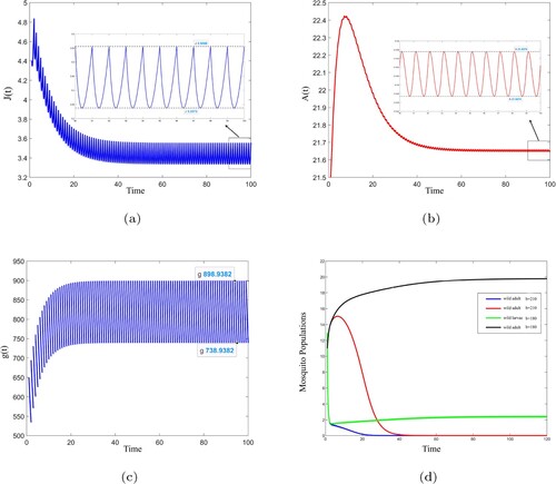Given the parameters $\begin{array}{rl}& \sigma =18,\alpha =7,d_0=0.35,d_1=0.3,{\mu }_1=0.25,{\mu }_2=0.196,\\ & r_0=68.5714,g_0=1738.2743,g_0^c=\mathrm{938.1150.}\end{array}$Figure 1 shows the number of mosquito larvae, mosquito adults and sterile mosquitoes changes with time. When T = 1, b = 160 with ${\overline{g}}_{max}=898.9382<g_0^c$(see Figure 1( a–c) in page 13), then according to theorem 3.3, we know that system (8(8) $\{\begin{array}{rl}& {\displaystyle \frac{\mathrm{d}J}{\mathrm{d}t}}={\displaystyle \frac{\sigma A}{A+g}}A-{\displaystyle \frac{\alpha J}{1+J}}-(d_0+d_{1}J)J,\\ & {\displaystyle \frac{\mathrm{d}A}{\mathrm{d}t}}={\displaystyle \frac{\alpha J}{1+J}}-{\mu }_{1}A,\\ & {\displaystyle \frac{\mathrm{d}g}{\mathrm{d}t}}=-{\mu }_{2}g,\\ & g(n{T}^{+})=g(nT)+b,\end{array}$(8) ) has two positive non-trivial periodic solutions $(J,A,g)=({\overline{J}}_1,{\overline{A}}_1,\overline{g})$ and $(J,A,g)=({\overline{J}}_2,{\overline{A}}_2,\overline{g})$, moreover $({\overline{J}}_1,{\overline{A}}_1,\overline{g})$ is an unstable non-trivial periodic solution $({\overline{J}}_2,{\overline{A}}_2,\overline{g})$ is a locally asymptotically stable non-trivial periodic solution. The calculated stable non-trivial periodic solution exists in the range $3.3373\le J\le 3.5558$, $21.6474\le A\le 21.6576$, $738.9382\le g\le 898.9382$. If T = 1, b = 210 with ${\overline{g}}_{max}=1179.7753<g_0$ and ${\overline{g}}_{min}=969.7753>g_0^c$ (see Figure 1(d) in page 13), then according to Theorem 3.3, we know that system (8(8) $\{\begin{array}{rl}& {\displaystyle \frac{\mathrm{d}J}{\mathrm{d}t}}={\displaystyle \frac{\sigma A}{A+g}}A-{\displaystyle \frac{\alpha J}{1+J}}-(d_0+d_{1}J)J,\\ & {\displaystyle \frac{\mathrm{d}A}{\mathrm{d}t}}={\displaystyle \frac{\alpha J}{1+J}}-{\mu }_{1}A,\\ & {\displaystyle \frac{\mathrm{d}g}{\mathrm{d}t}}=-{\mu }_{2}g,\\ & g(n{T}^{+})=g(nT)+b,\end{array}$(8) ) has no positive non-trivial periodic solution. If T = 1, b = 180 with ${\overline{g}}_{max}=1011.2359>g_0^c$ and ${\overline{g}}_{min}=831.2360<g_0^c$ (see Figure 1(d) in page 13), then theoretical analysis cannot get relevant conclusions. In this case, we can get that the periodic solution $({\overline{J}}_2,{\overline{A}}_2,\overline{g})$ is still stable according to the numerical simulation. It can be seen that when ${\overline{g}}_{min}<g_0^c<{\overline{g}}_{max}<g_0$, then system (8(8) $\{\begin{array}{rl}& {\displaystyle \frac{\mathrm{d}J}{\mathrm{d}t}}={\displaystyle \frac{\sigma A}{A+g}}A-{\displaystyle \frac{\alpha J}{1+J}}-(d_0+d_{1}J)J,\\ & {\displaystyle \frac{\mathrm{d}A}{\mathrm{d}t}}={\displaystyle \frac{\alpha J}{1+J}}-{\mu }_{1}A,\\ & {\displaystyle \frac{\mathrm{d}g}{\mathrm{d}t}}=-{\mu }_{2}g,\\ & g(n{T}^{+})=g(nT)+b,\end{array}$(8) ) can also exist two positive non-trivial periodic solutions.

Figure 1. (a–c) is the curve of the number of mosquito larvae, mosquito adults and sterile mosquitoes over time when T = 1, b = 160. (d) is the change curve of the number of mosquito larvae and adults when T = 1, b = 210 and T = 1, b = 180.

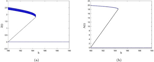
Next, we set the values of other parameters unchanged, and b is used as the bifurcation parameters to simulate the bifurcation of system (8(8) $\{\begin{array}{rl}& {\displaystyle \frac{\mathrm{d}J}{\mathrm{d}t}}={\displaystyle \frac{\sigma A}{A+g}}A-{\displaystyle \frac{\alpha J}{1+J}}-(d_0+d_{1}J)J,\\ & {\displaystyle \frac{\mathrm{d}A}{\mathrm{d}t}}={\displaystyle \frac{\alpha J}{1+J}}-{\mu }_{1}A,\\ & {\displaystyle \frac{\mathrm{d}g}{\mathrm{d}t}}=-{\mu }_{2}g,\\ & g(n{T}^{+})=g(nT)+b,\end{array}$(8) ). Given the parameters $\sigma =18,\alpha =7,d_0=0.35,d_1=0.3,{\mu }_1=0.25,{\mu }_2=0.196,T=1.$Figure 2 shows the bifurcation phenomenon of wild larvae $J(t)$(see Figure 2(a) in page 13) and wild adults $A(t)$(see Figure 2(b) in page 13) under the effects of sterile mosquitoes in system (8(8) $\{\begin{array}{rl}& {\displaystyle \frac{\mathrm{d}J}{\mathrm{d}t}}={\displaystyle \frac{\sigma A}{A+g}}A-{\displaystyle \frac{\alpha J}{1+J}}-(d_0+d_{1}J)J,\\ & {\displaystyle \frac{\mathrm{d}A}{\mathrm{d}t}}={\displaystyle \frac{\alpha J}{1+J}}-{\mu }_{1}A,\\ & {\displaystyle \frac{\mathrm{d}g}{\mathrm{d}t}}=-{\mu }_{2}g,\\ & g(n{T}^{+})=g(nT)+b,\end{array}$(8) ).

Figure 2. (a,b) shows the bifurcation phenomenon of system (8(8) $\{\begin{array}{rl}& {\displaystyle \frac{\mathrm{d}J}{\mathrm{d}t}}={\displaystyle \frac{\sigma A}{A+g}}A-{\displaystyle \frac{\alpha J}{1+J}}-(d_0+d_{1}J)J,\\ & {\displaystyle \frac{\mathrm{d}A}{\mathrm{d}t}}={\displaystyle \frac{\alpha J}{1+J}}-{\mu }_{1}A,\\ & {\displaystyle \frac{\mathrm{d}g}{\mathrm{d}t}}=-{\mu }_{2}g,\\ & g(n{T}^{+})=g(nT)+b,\end{array}$(8) ) when b is taken as the bifurcation parameter. The blue solid line represents the stable periodic solution, and the black dotted line represents the unstable period solution.

5. Concluding remarks

In this work, a stage-structured wild and sterile mosquito interaction impulsive model was formulated to investigate the effects of impulse release of sterile mosquitoes on the dynamics of wild mosquito populations. We assume that the environmental crowding only takes place in water where the egg, pupa, and larva stages in the life cycle of mosquitoes are present, and that the sterile mosquitoes are periodically released with the same amount.

In order to explore the effect of mosquito population suppression, we perform the dynamic analysis of the system. We first get the trivial periodic solution of the system. The trivial periodic solution is always locally asymptotically stable, and it is globally attractive under certain conditions. We then prove the existence conditions of non-trivial periodic solutions and their local stability. The system could exist two non-trivial periodic solutions, but only one of them is locally asymptotically stable. It is found that the system has the bistable phenomenon in which the trivial periodic solution and non-trivial periodic solution can coexist under certain threshold conditions. We finally verified the theoretical results with numerical simulations. Our dynamic results show that the appropriate releasing period and releasing the amount of sterile mosquitoes can control the wild mosquito population within a certain range, and even make them extinct.

Our paper gives a theoretical foundation for the Sterile Insect Technology (SIT) in the stage-structured impulsive model. All these results provide mosquito control practitioners with a theoretical basis for formulating the sterile mosquito release strategy. We believe this method could be used in other pest control such as Cylas formicarius or Drosophila, and other systems such as epidemiology or immunology.

Disclosure statement

Data sharing is not applicable to this article as no data sets were generated or analysed during the current study. The authors declare that they have no competing interests. No conflict of interest exists in the submission of this manuscript, and the manuscript is approved by all authors for publication. The authors would like to declare on that the work described was original research that has not been published previously, and not under consideration for publication elsewhere. All the authors listed have approved the manuscript that is enclosed.

Additional information

Funding

This work is supported by Natural Science Foundation of Jilin Province [grant number 20210101159JC] and the fund of the ‘Thirteen Five’ Scientific and Technological Research Planning Project of the Department of Education of Jilin Province [grant number JJKH20200726KJ].

References

- S. Ai, J. Li, J.S. Yu, and B. Zheng, Stage-structured models for interactive wild and periodically and impulsively released sterile mosquitoes, Discrete Contin. Dyn. Sys. B 27(6) (2022), pp. 3039–3052.
- D. Bainov and P. Simeonov, Impulsive Differential Equations: Periodic Solutions and Applications, CRC Press, Vol. 2, 1993. 26–30.
- H.J. Barclay, Pest population stability under sterile releases, Res. Popul. Ecol. (Kyoto) 24(2) (1982), pp. 405–416.
- H.J. Barclay, Modeling incomplete sterility in a sterile release program: Interactions with other factors, Popul. Ecol. 43(3) (2001), pp. 197–206.
- H. Barclay and M. Mackauer, The sterile insect release method for pest control: A density-dependent model, Environ. Entomol. 9(6) (1980), pp. 810–817.
- H.J. Barclay, Mathematical models for the use of sterile insects, Sterile Insect Technique, Springer, Dordrecht, 2005, pp. 147–174.
- P.-A. Bliman, D. Cardona-Salgado, Y. Dumont, and O. Vasilieva, Implementation of control strategies for sterile insect techniques, Math. Biosci. 314 (2019), pp. 43–60.
- L. Cai, S. Ai, and J. Li, Dynamics of mosquitoes populations with different strategies for releasing sterile mosquitoes, SIAM. J. Appl. Math. 74(6) (2014), pp. 1786–1809.
- A.N. Davis, J.B. Gahan, D.F. Weidhaas, and C.N. Smith, Exploratory studies on gamma radiation for the sterilization and control of Anopheles quadrimaculatus, J. Econ. Entomol. 52(5) (1959), pp. 868–870.
- V.A. Dyck and J.P. Hendrichs, Robinson, Sterile Insect Technique Principles and Practice in Area-Wide Integrated Pest Management, Springer, Dordrecht, 2005.
- K. Renee Fister, M.L. McCarthy, S.F. Oppenheimer, and C. Collins, Optimal control of insects through sterile insect release and habitat modification, Mathematical Biosciences 244(2) (2013), pp. 201–212.
- J.C. Flores, A mathematical model for wild and sterile species in competition: Immigration, Phys. A: Stat. Mech. Appl. 328(1–2) (2003), pp. 214–224.
- R.M. Gleiser, J. Urrutia, and D.E. Gorla, Effects of crowding on populations of Aedes albifasciatus larvae under laboratory conditions, Entomol. Exp. Appl. 95(2) (2000), pp. 135–140.
- J. Hendrichs, A.S. Robinson, J.P. Cayol, and W. Enkerlin, Medfly areawide sterile insect technique programmes for prevention, suppression or eradication: The importance of mating behavior studies, Florida Entomol 85(1) (2002), pp. 1–13.
- M.Z. Huang and X.Y. Song, Modelling and analysis of impulsive releases of sterile mosquitoes, J. Biol. Dyn. 11(1) (2017), pp. 147–171.
- D. Kaye, Breakthrough in mosquitopacked drones to combat Zika in Brazil, Clin. Infect. Dis. 2(67) (2018), pp. 2.
- A. Korobeinikov and G.C. Wake, Lyapunov functions and global stability for SIR, SIRS, and SIS epidemiological models, Appl. Math. Lett. 15(8) (2002), pp. 955–960.
- V. Lakshmikantham and P.S. Simeonov, Theory of Impulsive Differential Equations, World Scientific, 1989.
- J. Li, Simple stage-structured models for wild and transgenic mosquito populations, J. Diff. Equ. Appl. 15(4) (2009), pp. 327–347.
- J. Li, Malaria model with stage-structured mosquitoes, Math. Biosci. Eng. 8(3) (2011), pp. 753–768.
- J. Li, L. Cai, and Y. Li, Stage-structured wild and sterile mosquito population models and their dynamics, J. Biol. Dyn. 11(sup 1) (2017), pp. 79–101.
- Y.Z. Li and X.N. Liu, An impulsive model for Wolbachia infection control of mosquito-borne diseases with general birth and death rate functions, Nonlinear Anal Real World Appl 37 (2017), pp. 412–432.
- M.-T. Li, G.-Q. Sun, L. Yakob, H.-P. Zhu, Z. Jin, W.-Y. Zhang, and J. Ma, The driving force for 2014 dengue outbreak in Guangdong, China, PLos One 11(11) (2016), pp. e0166211.
- A. Meats, Demographic analysis of sterile insect trials with the Queensland fruit fly 'Bactrocera tryoni' (Froggatt) (Diptera: Tephritidae), Gen Appl Entomol 27 (1996), pp. 2–12.
- T.P. Monath, Dengue: the risk to developed and developing countries, Proc. Natl. Acad. Sci. 91(7) (1994), pp. 2395–2400.
- S. Moriya and T. Miyatake, Eradication programs of two sweetpotato pests, Cylas formicarius and Euscepes postfasciatus, in Japan with special reference to their dispersal ability, Jpn Agric. Res. Quart. 35(4) (2001), pp. 227–234.
- S. Nundloll, L. Mailleret, and F. Grognard, Two models of interfering predators in impulsive biological control, J. Biol. Dyn. 4(1) (2010), pp. 102–114.
- D.L. Scarnecchia, Mosquitoes and their control, Ann. Trop. Med. Parasitol. 104(6) (2003), pp. 687–688.
- C.M. Stone and M. Somers, Transient population dynamics of mosquitoes during sterile male releases: Modelling mating behaviour and perturbations of life history parameters, PLoS ONE 8(9) (2013), pp. e76228.
- E. Waltz, US government approves 'killer' mosquitoes to fight disease, Nature. (2017), pp. 22959.
- S. Wang and Q.D. Huang, The sterile insect release technique in a predator-prey system with monotone functional response, Electron. J. Qual. Theory. Differ. Equ. 2016 (2016), pp. 1–20.
- W. Yiguan, L. Xin, L. Chengling, T. Su, J. Jianchao, G. Yuhong, R. Dongsheng, Y. Zhicong, L. Qiyong, and M. Fengxia, A survey of insecticide resistance in Aedes albopictus (Diptera: Culicidae) during a 2014 dengue fever outbreak in Guangzhou, China, J. Econ. Entomol. 110(1) (2017), pp. 239–244.
- S.M. White, P. Rohani, and S.M. Sait, Modelling pulsed releases for sterile insect techniques: Fitness costs of sterile and transgenic males and the effects on mosquito dynamics, J. Appl. Ecol. 47(6) (2010), pp. 1329–1339.
- L. Yakob, L. Alphey, and M.B. Bonsall, Aedes aegypti control: The concomitant role of competition, space and transgenic technologies, J. Appl. Ecol. 45(4) (2008), pp. 1258–1265.
- J.S. Yu, Modeling mosquito population suppression based on delay differential equations, SIAM. J. Appl. Math. 78(6) (2018), pp. 3168–3187.
- J.S. Yu, Existence and stability of a unique and exact two periodic orbits for an interactive wild and sterile mosquito model, J. Differ. Equ. 269(12) (2020), pp. 10395–10415.
- J.S. Yu and J. Li, A delay suppression model with sterile mosquitoes release period equal to wild larvae maturation period, J. Math. Biol. 84(3) (2022), pp. 1–19.
- X. Zhang, Q. Liu, and H. Zhu, Modeling and dynamics of Wolbachia-infected male releases and mating competition on mosquito control, J. Math. Biol. 81 (2020), pp. 243–276.
- X. Zhang, S. Tang, R.A. Cheke, and H. Zhu, Modeling the effects of augmentation strategies on the control of dengue fever with an impulsive differential equation, Bull. Math. Biol. 78(10) (2016), pp. 1968–2010.
- X. Zhang, S. Tang, Q. Liu, R.A. Cheke, and H. Zhu, Models to assess the effects of non-identical sex ratio augmentations of Wolbachia-carrying mosquitoes on the control of dengue disease, Math Biosci 299 (2018), pp. 58–72.
- B. Zheng, J.S. Li, and J. Yu, Existence and stability of periodic solutions in a mosquito population suppression model with time delay, J. Differ. Equ. 315 (2022), pp. 159–178.
- B. Zheng, J.S. Yu, and J. Li, Modeling and analysis of the implementation of the Wolbachia incompatible and sterile insect technique for mosquito population suppression, SIAM. J. Appl. Math. 81(2) (2021), pp. 718–740.
- X. Zheng, D. Zhang, Y. Li, C. Yang, Y. Wu, X. Liang, Y. Liang, X. Pan, L. Hu, Q. Sun, X. Wang, Y. Wei, J. Zhu, W. Qian, Z. Yan, A. G. Parker, J.R.L. Gilles, K. Bourtzis, J. Bouyer, M. Tang, B. Zheng, J. Yu, J. Liu, J. Zhuang, Z. Hu, M. Zhang, J.-T. Gong, X.-Y. Hong, Z. Zhang, L. Lin, Q. Liu, Z. Hu, Z. Wu, L.A. Baton, A.A. Hoffmann, and Z. Xi, Incompatible and sterile insect techniques combined eliminate mosquitoes, Nature 572 (2019), pp. 56–61.
- Z. Zhu, B. Zheng, Y. Shi, R. Yan, and J. Yu, Stability and periodicity in a mosquito population suppression model composed of two sub-models, Nonlinear. Dyn. 107(1) (2021), pp. 1383–1395.