
 ?Mathematical formulae have been encoded as MathML and are displayed in this HTML version using MathJax in order to improve their display. Uncheck the box to turn MathJax off. This feature requires Javascript. Click on a formula to zoom.
Abstract
In this study, a model for the spread of cyst echinococcosis with interventions is formulated. The disease-free and endemic equilibrium points of the model are calculated. The control reproduction number for the model is derived, and the global dynamics are established by the values of
. The disease-free equilibrium is globally asymptotically stable if and only if
. For
, using Volterra–Lyapunov stable matrices, it is proven that the endemic equilibrium is globally asymptotically stable. Sensitivity analysis to identify the most influential parameters in the dynamics of CE is carried out. To establish the long-term behaviour of the disease, numerical simulations are performed. The impact of control strategies is investigated. It is shown that, whenever vaccination of sheep is carried out solely or in combination with cleaning or disinfecting of the environment, cyst echinococcosis can be wiped out.
1. Introduction
Cystic echinococcosis (CE) is caused by the tapeworm belonging to the family Taeniidae, called Echinococcus granulosus (for more detail, see [Citation3,Citation9,Citation11,Citation26]). Echinococcus granulosus organisms take part in both asexual reproduction and sexual reproduction. Asexual reproduction takes place via budding in the intermediate host, while sexual reproduction takes place by gamete fusion in the definitive host. Echinococcus granulosus is hermaphroditic, containing both male and female sex organs. The transmission dynamics of the disease depends on a number of factors. These include the parasite's biotic potential, stimulation of immunity in life cycle hosts, life expectancy and development time of the parasite. Social and ecological factors such as meat inspection practices, disposal of offal and casualty animals and populations of stray, feral or sylvatic hosts can all affect transmission of this parasite [Citation26]. Consuming offal containing E. granulosus by definite hosts can lead to infection. The frequency of offal feedings and the prevalence of the parasites within the offal are factors that affect infection pressure within the definitive host. The immunity of both the definitive and intermediate host plays a large role in the transmission of the parasite, as well as the contact rate between the intermediate and the definitive host (such as herding dogs and pasture animals being kept in close proximity where dogs can contaminate grazing areas with fecal matter) [Citation21]. The environment plays a powerful role in the transmission of infectious diseases. As that of many environmental disease, cystic echinococcosis is affected by various biological and environmental factors [Citation12,Citation23].
Infection with E. granulosus remains a major public health issue in several countries and regions, even in places where it was previously at low levels, as a result of a reduction of control programmes due to economic problems and lack of resources [Citation13]. Although control programmes against human cystic (CE), caused by E. granulosus, have been established in some countries and effective control strategies are available, the parasite has still affected many countries of all continents. Thus human CE is persisting in many parts of the world with high incidences [Citation9,Citation13]. The human incidence can exceed 50 per 100,000 person-years in areas of endemicity, and prevalence rates as high as 5–10% can be found in some countries [Citation14]. The incidence of human Hydatid disease in any country is closely related to the prevalence of the disease in domestic animals and is highest where there is a large dog population and high sheep production [Citation7]. The average annual death rate from echinococcosis is 0.007 per 10,000 population, which is very low. The main causes of death are either complications of hepatic and pulmonary echinococcosis or echinococcosis of the heart. The complications of liver echinococcosis may develop due to the changes occurring not only in the parasitic cyst but also in the affected organ or in the patient's body [Citation15].
According to WHO, cystic echinococcosis is a preventable disease [Citation22]. To employ preventive measures, understanding of the transmission dynamics, both between dogs and sheep where the parasite maintains itself and from dogs to human is important. It is from this knowledge that effective control measures can be devised to reduce the prevalence of the parasite in animals and hence reduce the incidence of human disease. Understanding of the epidemiology of echinococcosis has been greatly improved, new diagnostic techniques for both humans and animals have been developed, new prevention strategies have emerged with the development of a vaccine against E. granulosus in intermediate hosts[Citation9]. Since sheep has a substantial potential to transmission of parasite, vaccination of sheep with an E. granulosus recombinant antigen (EG95) offers encouraging prospects for prevention and control [Citation5]. The vaccine is currently being produced commercially and is registered in China and Argentina. Trials in Argentina demonstrated the added value of vaccinating sheep, and in China the vaccine is being used extensively [Citation1,Citation7]. Currently there are no human vaccines against any form of echinococcosis [Citation1].
Echinococcus eggs can be inactivated by disinfectants such as formalin, chlorine gas, certain freshly-prepared iodine solutions (but not most iodides) or lime can inhibit hatching of the embryo and reduce the number of viable eggs. Food safety precautions such as thorough washing of fruits and vegetables, combined with good hygiene, can reduce exposure to eggs on food. The hands should always be washed after handling pets or farming, gardening or preparing food, and before eating. Water from unsafe sources such as lakes should be boiled or filtered. Meat, particularly the intestinal tract of carnivores, should be thoroughly cooked before eating. PPE reduces the risk of infection when working with animal tissues or fecal samples and periodic surveillance of high-risk populations [Citation10].
In [Citation5], a mathematical model of the transmission dynamics of cyst echinococcosis without intervention was presented and analysed. From the result of sensitivity analysis, it was found that the transmission rate of E. granulosus eggs from the environment to sheep is the most influential parameter that control the dynamics of disease. Thus the prevention of the disease depends on the interruption of the life cycle of E. granulosus. To break the parasite's life cycle and control the disease transmission, vaccination of sheep and/or cleaning of environment are practical alternatives.
In this paper, the model developed in [Citation5] is extended by incorporating vaccination of sheep and disinfection or cleaning of the environment as control strategies. The objective of this paper is to determine the better control method from vaccination of sheep and disinfection or cleaning of environment.
The rest of this paper is organized as follows. In Section 2, mathematical model of cyst echinococcosis with intervention is presented. In Section 3, the positivity and boundedness of solutions are discussed. In Section 4, both the disease free and endemic equilibrium points are determined, local and global stability of these equilibrium points with the calculation of the control reproduction number are presented. Moreover, local and global sensitivity analyses, numerical simulations and effects of control strategies are presented in Section 5, and finally conclusion is drawn in Section 6.
2. Model formulation
We formulate a compartmental model to describe the transmission dynamics of the disease by considering the dog, sheep and human populations. The total populations of dog, sheep and human are assumed constant, and denoted by ,
and
respectively, so that the birth rate and death rate of each of the populations are equal. The dog population has three classes: the Susceptible (
), Exposed (
) and Infectious (
) classes. The human population has four classes: the Susceptible (
), Exposed (
), Infectious (
) and Removed (
) classes. The sheep population has four classes: the Susceptible (
), Exposed (
), Infectious (
) and Vaccinated (
) classes. Dog, sheep and human populations are recruited to susceptible class by birth at rates
,
and
respectively.
The transmission cycle of E. granulosus involves two hosts (dogs and sheep) and free living stages. The relative times spent in the different stages of the life cycle of the parasite and the hosts are of considerable importance to the analysis of model behaviour. The sexual reproduction of the parasites in the dog population is an important factor for the load of the parasite. The concentration of the parasite in the environment is increased by shedding from infected dog at a rate and decreased by the natural death rate of E. granulosus eggs at rate
and disinfection or cleaning of environment at rate μ, where
denote the mean number of parasite per dog host. Although modelling infectious diseases that are caused by parasites is best formulated using the intensity of infection which measures the number of parasites rather than the prevalence of infection [Citation18], in this work, we considered the latter. Here, the incidence function represents sufficient number of parasites that can cause infection as reported in [Citation30]. Thus the time evolution of the parasite egg's is represented by the following differential equation:
In the dynamics of the disease transmission, susceptible sheep are infected by ingesting parasite eggs in the feces of infected definitive hosts (dogs), while humans are infected by accidentally ingesting E. granulosus eggs from the environment. We introduced vaccination to the susceptible sheep population at a rate ν, so that the population of susceptible sheep is reduced through vaccination and moved to vaccinated
class. We assume that vaccination is not lifelong. The sheep population may lose of vaccine-induced immunity and move back to susceptible class at a rate ρ. Rate of infection of susceptible sheep is
, where
denotes the rate of ingestion of Echinococcus egg from the environment by sheep and
is the half-saturation constant of parasite in the environment sufficient to infect sheep. Rate of infection of susceptible humans is
, where
denotes the rate of ingestion of Echinococcus egg from the environment by human, and
is the half-saturation constant of parasite in the environment sufficient to infect human. Susceptible dogs are infected by preying on the infected sheep. The disease transmission rate from sheep to dogs is denoted by
. The rates at which exposed dog, sheep and human progress to infectious classes are denoted by
,
and
respectively. Infected human population could recover from the disease naturally, at rate
, whereas sheep and dogs cannot recover once they are infected. We assume that there is no echinococcus induced death. However, dogs, sheep and humans die naturally at rates
,
and
respectively. The density of E. granulosus eggs depends mainly on the number of infectious dogs. Its concentration in the environment is increased by shedding of a parasite from infected dog at a rate δ and decreased by the natural death rate of E. granulosus eggs at rate
and disinfection or cleaning of environment at rate μ.
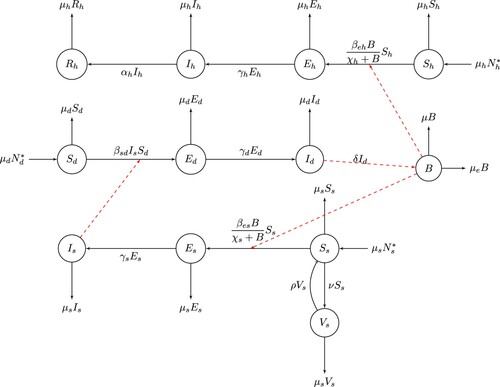
The general structure of the model is captured by the flow chart displayed in Figure .
Figure 1. The flow diagram for cyst echinococcosis transmission dynamics.
The transmission dynamics of the disease in the three populations can now be expressed by the following system of first-order differential equations:
(1)
(1)
(2)
(2)
(3)
(3)
(4)
(4)
(5)
(5)
(6)
(6)
(7)
(7)
(8)
(8)
(9)
(9)
(10)
(10)
(11)
(11)
(12)
(12)
with initial conditions
,
,
,
,
,
,
,
,
,
,
and
.
For convenience, we make the following substitutions: ,
,
and
. Thus we can rewrite the system (Equation1
(1)
(1) )–(Equation12
(12)
(12) ) with initial conditions as
(13)
(13)
where
,
defined by
3. Well-posedness of the solutions
Before we proceed with the mathematical analysis, we need to show that the models (Equation1(1)
(1) )–(Equation12
(12)
(12) ) (alternatively model (Equation13
(13)
(13) )) is well-posed epidemiologically and mathematically in a feasible domain.
Theorem 3.1
The region , where
,
,
and
is positively invariant for models (Equation1
(1)
(1) )–(Equation12
(12)
(12) ).
Proof.
Proof of this theorem is presented in Appendix 1
4. Existence and stability of equilibria
The equilibrium point(s) of the system (Equation1(1)
(1) )–(Equation12
(12)
(12) ) are obtained by equating the right hand sides to zero as follows:
(14a)
(14a)
(14b)
(14b)
(14c)
(14c)
(14d)
(14d)
(14e)
(14e)
(14f)
(14f)
(14g)
(14g)
(14h)
(14h)
(14i)
(14i)
(14j)
(14j)
(14k)
(14k)
(14l)
(14l)
From Equations (Equation14c
(14c)
(14c) ) and (Equation14d
(14d)
(14d) ), we respectively have
(15a)
(15a)
From Equations (Equation14a
(14a)
(14a) ), (Equation14b
(14b)
(14b) ) and using (Equation15a
(15a)
(15a) ) we have
(15b)
(15b)
Substituting (Equation15b
(15b)
(15b) ) in (Equation14a
(14a)
(14a) ) yields
(15c)
(15c)
Similarly, from Equations (Equation14i
(14i)
(14i) )–(Equation14l
(14l)
(14l) ), we obtain
(15d)
(15d)
By Equating (Equation15c
(15c)
(15c) ) and (Equation15d
(15d)
(15d) ), we then obtain a quadratic equation
(16)
(16)
where
and
Thus we have two roots
(17)
(17)
The results presented in Sections 4.1 and 4.4 follow from these two roots.
4.1. Disease-free equilibrium (DFE)
From algebraic computation when B = 0, the system (Equation13(13)
(13) ) has the DFE given by
4.2. The control reproduction number
A key quantity in epidemiological models is the reproduction number. It is a useful threshold in the study of a disease for predicting outbreak and for evaluating the control strategies. Due to the presence of controls in the model (Equation13(13)
(13) ), the term ‘the control reproduction number’ is used. The control reproduction number, denoted by
represents the average number of secondary infections caused by an infectious individual over the course of infectious period in a totally susceptible population under specified controls. We derive the control reproduction number
by using the Next Generation Matrix (NGM) approach [Citation27] on the system (Equation13
(13)
(13) ). The detail computation is done in Appendix A. Thus the control reproduction number is given by
where
is the basic reproduction number as derived in [Citation5], which represents the average number of secondary infections caused by an infectious individual over the course of infectious period in a totally susceptible population without vaccination and disinfection or cleaning of the environment. Here, we can notice that
.
4.3. Stability of the DFE
Theorem 4.1
If , then the disease free equilibrium
is globally asymptotically stable in
. If
, then the DFE is unstable, the system is persistent and there is at least one equilibrium in the interior of
.
Proof.
To prove the global stability of the disease free equilibrium , we use a matrix-theoretic method as explained in [Citation25].
The disease compartments of model (Equation13(13)
(13) ) can be written as
where
,
, F and V are matrices given in (EquationA1a
(A1a)
(A1a) ) and (EquationA1b
(A1b)
(A1b) ), and
since
,
,
, and
.
Matrices F and are entry wise non negative with
Since
is reducible matrix [Citation4], the condition of Theorem 2.2 in [Citation25] fails. Instead, to establish the global stability of the DFE, we construct a Lyapunov function by using Theorem 2.1 of [Citation25].
Let be the left eigenvector of
corresponding to the eigenvalue
. Thus
As a result, we found that
is the left eigenvector of
corresponding to the eigenvalue
. Thus by Theorem 2.1 of [Citation25],
is a Lyapunov function for model (Equation1
(1)
(1) )–(Equation12
(12)
(12) ). Then differentiating along the solutions of the system (Equation1
(1)
(1) )–(Equation12
(12)
(12) ) gives
(18)
(18)
Since
,
and
,
if
. If
, then B = 0 and
. Hence, the largest invariant set of the model where
in
is the singleton
. Therefore, by Lasalle's invariance principle [Citation16], the disease free equilibrium
is globally asymptotically stable if
. For
, the first term in (Equation18
(18)
(18) ) is positive in
, and the remaining terms are equal to zero when B = 0 and
, where
and
. Consequently,
in a neighbourhood of
. Thus the disease free equilibrium
is unstable, and using Theorem 2.2 of [Citation25], the system (Equation13
(13)
(13) ) is uniformly persistent and hence imply there is at least one endemic equilibrium in the interior of
.
4.4. Existence and stability of the endemic equilibrium (EE)
From (Equation17(17)
(17) ), it follows that the model (Equation13
(13)
(13) ) admits an endemic equilibrium. Thus the endemic equilibrium point of the system in terms of the control reproduction number
is given by
where
(19a)
(19a)
(19b)
(19b)
(19c)
(19c)
(19d)
(19d)
(19e)
(19e)
(19f)
(19f)
(19g)
(19g)
(19h)
(19h)
(19i)
(19i)
(19j)
(19j)
(19k)
(19k)
(19l)
(19l)
For
, it can be noted that the endemic equilibrium point reduces to disease free equilibrium point. Under the condition
, the quadratic equation (Equation17
(17)
(17) ) has no positive root. Hence, the model equation (Equation13
(13)
(13) ) has no positive endemic equilibrium whenever
. This consequently indicates that the backward bifurcation phenomenon does not occur whenever
. On the contrary, the disease will persist if
exceeds unity, where a stable endemic equilibrium exists. The phenomenon, where the disease-free equilibrium loses its stability and a stable endemic equilibrium appears as
increases through one, is known as forward bifurcation.
Theorem 4.2
If , then an endemic equilibrium
defined by Equations (Equation19a
(19a)
(19a) )–(Equation19l
(19l)
(19l) ) is globally asymptotically stable, and the bifurcation of endemic equilibrium point is forward when
.
Proof.
Detailed proof of this theorem is presented in Appendix 3.
5. Numerics: elasticity indices, numerical simulations and control strategies
5.1. Elasticity indices
In this section, we carried out sensitivity analysis to determine the model robustness to parameter values. This is a tool to identify the most influential parameters in determining model dynamics. Sensitivity analysis is used to obtain the sensitivity index that is a measure of the relative change in a state variable when a parameter changes. We compute the sensitivity indices of to the model parameters with the approach used by Chitnis et al. [Citation6,Citation20]. These indices could be computed numerically so as to figure out parameters that have high impact on control reproduction number
, and the importance of each individual parameter in the disease transmission dynamics and prevalence. To perform the local sensitivity analysis, we use the normalized forward sensitivity index of a variable with respect to a parameter which is expressed as the ratio of the relative variation in the variable to the relative variation in the parameter. Thus the normalized forward sensitivity index (elasticity index) of a variable (
) with respect to a parameter p is the ratio of the relative change in the variable to the relative change in the parameter, given by
We use data from the literature, and due to the great variation of some parameter values from region to region, without deviation from the range of parameter values obtained from literature, assumed (estimated) values were used for sensitivity analysis, as given in Table . The parameter values were hypothetically chosen, because the intention for this work is not to validate the model results of the real situation obtained in a particular study, but for illustrative purposes only. With sensitivity analysis, we can get insight into the appropriate intervention strategies to prevent and control the spread of the disease.
Table 1. Parameters, baseline values and sources.
Sensitivity indices of the control reproduction number with respect to the model nine parameters are determined and presented in the table below. Ranges of these parameters are taken without deviation to the data obtained in the literature and assumed values. Natural birth rates and death rates of the populations are not considered for sensitivity analysis since these parameters are difficult to control.
Table gives the elasticity indices of with respect to key parameters of model (Equation1
(1)
(1) )–(Equation12
(12)
(12) ) at the baseline values indicated in Table and arranged in descending order of magnitudes. The sign of the elasticity index tells whether
increases (positive sign) or decreases (negative sign) with the parameter, whereas the magnitude determines the relative importance of the parameter. From the magnitude of elasticity index, we can notice that four parameters
have equal and the greatest influence for the transmission of the disease, followed by
,
and ν, and ρ has the least influence for the transmission of the disease.
Table 2. Elasticity indices of relative to some model parameters.
5.2. Global sensitivity analysis
From the local sensitivity analysis, we observed that it is impossible to differentiate explicitly the most influential parameter(s) of the model. To determine which parameter(s) among the nine is (are) most influential in the dynamics of the disease, global sensitivity analysis is done. We employed the technique of Latin Hypercube Sampling (LHS) to test the sensitivity of the model to each input parameter, as described and implemented in [Citation19], and Partial Rank Correlation Coefficients (PRCCs) to assess the significance of each parameter with respect to each metric is used. Latin hypercube sampling is a stratified sampling technique that creates sets of parameters by sampling for each parameter according to a predefined probability distribution. To examine the dependence of on parameter variations, we determine the PRCC values by considering a range of parameters as given in Table , with sample size 1000. The result is depicted in Figure . The parameter with PRCC value far away from zero indicates the more strongly the parameter influence
. The negative sign for PRCCs indicates inverse proportionality.
Figure 2. Global sensitivity analysis displaying the partial rank correlation coefficients (PRCC) of control reproduction number .
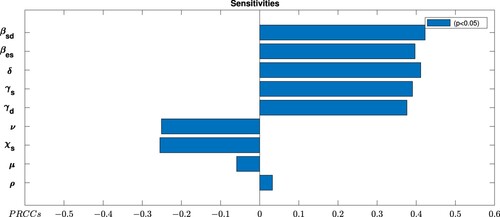
From Figure , it is observed that the transmission rate from sheep to dog () and Echinococcos eggs contamination rate of the environment by infected dogs (δ) are the most influential parameters among the eight parameters in the disease dynamics. On the other hand, rate of losing vaccine induced immunity of sheep are the least sensitive parameter for the dynamics of the disease.
5.3. Numerical simulations
In this section, we carry out numerical simulations for mathematical model of cyst echinococcosis in the populations of sheep, dogs and humans. We use the total populations ,
,
, and parameter values given in Table . This yields a control reproduction number
. Using different initial conditions, the time evolution of human, sheep and dog populations for model (Equation13
(13)
(13) ) is displayed in Figure . We can notice that all disease compartments
,
,
,
,
,
,
and
converge asymptotically to zero, while the noninfected compartments
,
and
converge to their respective total populations. This asserts the global stability of the disease free equilibrium as proved in Theorem 4.1.
Figure 3. Time evolution of the dog, sheep and human populations with baseline parameter values as in Table , using different initial conditions which gives .
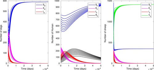
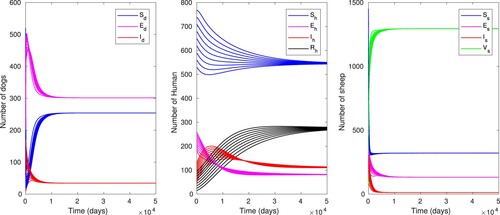
Figure shows that the time evolution of human, sheep and dog populations for model (Equation13(13)
(13) ) with parameter values given in Table by increasing
to
. In this case, the control reproductive number is
, and depict the global stability of the endemic equilibrium as proved in Theorem 4.2. It can be noticed that all the compartments of the dog, human and sheep populations converge asymptotically to their respective endemic equilibrium points irrespective of any initial conditions.
Figure 4. Time evolution of the dog, sheep and human populations with baseline parameter values as in Table , using different initial conditions, except for which gives
, and with approximate equilibrium values
,
,
,
,
,
,
,
,
,
,
.
In the case of endemicity, the prevalence rate of human is
The prevalence rate resulted in the numerical simulation is higher than the WHO published data, since the WHO report showed that the human prevalence rate is 5–10% (as indicated in [Citation14]). This result has shown at least 8.9% discrepancy from WHO published data.
5.4. Effects of control strategies on 
The numerical simulations are performed to illustrate the effect of vaccination of sheep and cleaning or disinfecting the environment in the dynamics of the disease transmission in the populations of sheep, dogs and humans while they are used alone or simultaneously.
The effect of vaccination of sheep using baseline parameter values in Table except for , and when ν is varied from
to 0.005, is displayed in Figure . As a result the infectious sheep, dog and human populations are respectively reduced from 25 to 0, 13 to 0, and 80 to 0, where the control reproduction number is also reduced from
to
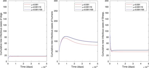
. This result shows that increasing the rate of vaccination of sheep (ν) reduces the time evolution of infected human, sheep and dog populations. The effect of disinfection or cleaning the environment using baseline parameter values in Table except for
, and when μ is varied from
to 0.001, is displayed in Figure . As a result the infectious sheep, dog and human populations are respectively reduced from 37 to 32, 18 to 16 and 93 to 79, where the control reproduction number is also reduced from
to
. This result shows that increasing the rate of disinfection or cleaning the environment (μ) has very less effect to eradicate the disease transmission in human, sheep and dog populations.
Figure 5. The numerical simulations displaying effects of vaccination of sheep only on cumulative number of infectious dog, human and sheep populations, using parameter values in Table , with varying values of ν ().
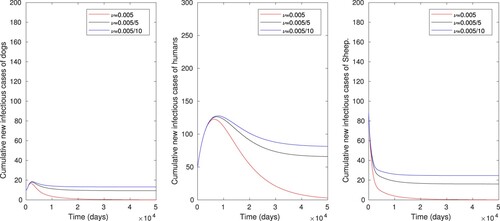
Figure 6. The numerical simulations displaying effects of disinfection or cleaning the environment only on cumulative number of infectious dog, human and sheep populations, using parameter values in Table , with varying values of μ ().
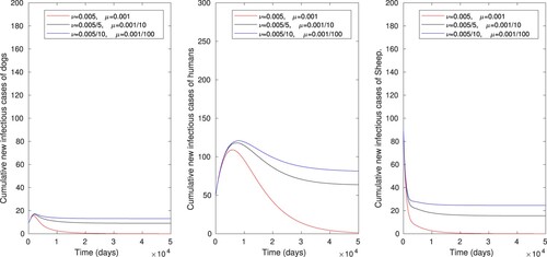
Numerical simulation is also performed to illustrate the effect of vaccination of sheep and disinfection or cleaning the environment when the two control strategies are administered simultaneously, as displayed in Figure . The number of infectious sheep, dog and human populations are respectively reduced from 26 to 0, 13 to 0 and 80 to 0, where the control reproduction number is also reduced from to
. One can observe that these combined effects allow to reduce the size of infected individuals. Thus increasing the vaccination rate of sheep alone or a simultaneous increase of the vaccination rate of sheep and rate of cleaning or disinfecting the environment is an effective control measure of cyst trichinosis.
Figure 7. The numerical simulations displaying effects of combining controlling strategies on cumulative number of infectious dog, human and sheep populations, using parameter values in Table .
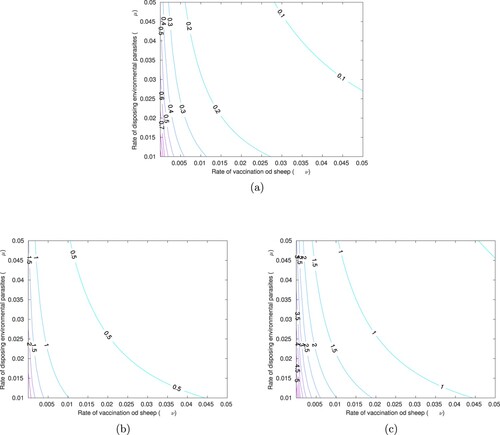
Furthermore, we assess the impact of combined control strategies using contour plots of as function of the control strategies, and with varying rate of transmission from sheep to dog (
), we estimate the least values of the two control parameters which will ensure the disease eradication in the populations.
Figure (a) shows contour curves of as a function of ν and μ using baseline parameter values in Table . We can observe that, low control strategies are needed to ensure the eradication of the parasites, with range of
and mean
. Contour plots of
as function of the control strategies, for rate of transmission from sheep to dog (
) is displayed in Figure (b). The least values of ν and μ that will ensure parasites eradication are estimated to be 0.01 and 0.01 so that
. In this case, the combined control strategies have effect in the disease transmission with range of
and mean
. Contour plots of
as function of the control strategies, for rate of transmission from sheep to dog (
) is displayed in Figure (c).The least values of ν and μ that will ensure parasites eradication are estimated to be 0.045 and 0.01 so that
. In this case, the combined control strategies has effect in the disease transmission with range of
and mean
. These results have shown that a remarkable increase in the control reproduction number is observed with an increase rate of transmission from sheep to dog (
). Hence, to ensure the eradication of parasites, we must introduce the least values of the controls that can bring the value
with respect to the rate of transmission from sheep to dog (
).
Figure 8. Contour curves of as a function of ν and μ using different rate of transmission from sheep to dog (
) with (a) parameter values in Table , (b)
, (c)
.
6. Conclusion
In this paper, we proposed and analysed a deterministic model for transmission dynamics of cyst trichinosis that incorporates two control strategies namely vaccination of sheep and disinfection or cleaning the environment. The model has a Disease Free Equilibrium point (DEF) which is both locally and globally asymptotically stable whenever the control reproduction number . We also found the Endemic Equilibrium points (I) and proved that it is globally stable whenever the control reproduction number
. Moreover, we have performed sensitivity analysis on the control reproduction number with the two control strategies, from which we have noted that the most sensitive parameters are the transmission rate from sheep to dog (
) and Echinococcus eggs contamination rate of the environment by infected dogs (δ). Numerical simulations of the model have shown that whenever the control strategies are carried out solely then vaccination of sheep is the better alternative to eradicate cyst echinococcosis, but when disinfection or cleaning the environment is carried out solely, its effect to eradicated the disease is very less. This indicates that to eradicate the disease from the three populations the model needs to incorporate other possible intervention strategies that can reduce
. Our finding has shown that the two control strategies are not enough to control the disease. We suggest that more controls, which focus more on dog population, should be incorporated to eradicate the spread of cyst echinococcosis. In our future, we will extend the model by incorporating additional control(s) and investigate the effectiveness and cost effectiveness of the control measures.
Disclosure statement
The authors declare that there is no conflict of interests regarding the publication of this paper.
Data availability
The numerical data used in our research are obtained from the published literature, which are cited therein. We also use reasonable estimate, for the data that are not available in the literature.
References
- J.-A.M. Atkinson, G.M. Williams, L. Yakob, A.C.A. Clements, T.S. Barnes, D.P. McManus, Y.R. Yang, D.J. Gray and A.L. Willingham, Synthesising 30 years of mathematical modelling of echinococcus transmission, PLoS Negl Trop Dis 7(8) (2013), pp. e2386.
- R. Azlaf and A. Dakkak, Epidemiological study of the cystic echinococcosis in Morocco, Vet. Parasitol. 137(1–2) (2006), pp. 83–93.
- C. Benner, H. Carabin, L.P. Sánchez-Serrano, C.M. Budke and D. Carmena, Analysis of the economic impact of cystic echinococcosis in Spain, Bull. World. Health. Organ. 88 (2010), pp. 49–57.
- A. Berman and R.J. Plemmons, Nonnegative Matrices in the Mathematical Sciences, SIAM, Vol. 9, 1994.
- G.B. Birhan, J.M.W. Munganga, A.S. Hassan and F. Hartung, Mathematical modeling of echinococcosis in humans, dogs, and sheep, J. Appl. Math. 2020 (2020), pp. 1–18.
- N. Chitnis, J.M. Hyman and J.M. Cushing, Determining important parameters in the spread of malaria through the sensitivity analysis of a mathematical model, Bull. Math. Biol. 70(5) (2008), pp. 1272–1296.
- P. S Craig, D.P McManus, M.W Lightowlers, J.A Chabalgoity, H.H Garcia, C.M Gavidia, R.H Gilman, A.E Gonzalez, M. Lorca, C. Naquira, A. Nieto and P.M Schantz, Prevention and control of cystic echinococcosis, The Lancet Infectious Diseases 7(6) (2007), pp. 385–394.
- O. Diekmann, J.A.P. Heesterbeek and J.A. Metz, On the definition and the computation of the basic reproduction ratio R0 in models for infectious diseases in heterogeneous populations, J. Math. Biol. 28(4) (1990), pp. 365–382.
- J. Eckert, M. Gemmell, F.-X. Meslin, Z. Pawlowski, and W H Organization, WHO/OIE manual on echinococcosis in humans and animals: a public health problem of global concern, 2001.
- T. C. for food Security and P. Health. Echinococcosis, echinococciasis, hydatidosis, hydatid disease.
- M. Gemmell, J. Lawson and M. Roberts, Population dynamics in echinococcosis and cysticercosis: evaluation of the biological parameters of Taenia hydatigena and T. ovis and comparison with those of echinococcus granulosus, Parasitology 94(1) (1987), pp. 161–180.
- M.A. Ghatee, K. Nikaein, W.R. Taylor, M. Karamian, H. Alidadi, Z. Kanannejad, F. Sehatpour, F. Zarei and G. Pouladfar, Environmental, climatic and host population risk factors of human cystic echinococcosis in southwest of iran, BMC. Public. Health. 20(1) (2020), pp. 1–13.
- G. Grosso, S. Gruttadauria, A. Biondi, S. Marventano and A. Mistretta, Worldwide epidemiology of liver hydatidosis including the Mediterranean area, World Journal of Gastroenterology: WJG 18(13) (2012), pp. 1425.
- N.I.A. Higuita, E. Brunetti, C. McCloskey, and C.S. Kraft, Cystic echinococcosis, J. Clin. Microbiol. 54(3) (2016), pp. 518–523.
- A.S. Khachatryan, Analysis of lethality in echinococcal disease, Korean. J. Parasitol. 55(5) (2017), pp. 549–553.
- J.P. LaSalle, The Stability of Dynamical Systems, Siam, Vol. 25, 1976.
- S. Liao and J. Wang, Global stability analysis of epidemiological models based on Volterra–Lyapunov stable matrices, Chaos Sol. Fract. 45(7) (2012), pp. 966–977.
- G. Macdonald, Epidemiologic models in studies of vector-borne diseases: the re dyer lecture, Public. Health. Rep. 76(9) (1961), pp. 753–00.
- S. Marino, I.B. Hogue, C.J. Ray and D.E. Kirschner, A methodology for performing global uncertainty and sensitivity analysis in systems biology, J. Theor. Biol. 254(1) (2008), pp. 178–196.
- M. Martcheva, An Introduction to Mathematical Epidemiology, Springer, Vol. 61, 2015.
- P. Moro, J. McDonald, R.H. Gilman, B. Silva, M. Verastegui, V. Malqui, G. Lescano, N. Falcon, G. Montes and H. Bazalar, Epidemiology of Echinococcus granulosus infection in the central peruvian andes, Bull. World. Health. Organ. 75(6) (1997), pp. 553.
- W. H. ORGANIZATION, Neglected tropical diseases, echinoccocosis.
- S. Osman, O.D. Makinde and D.M. Theuri, Mathematical modelling of listeriosis epidemics in animal and human population with optimal control, Tamkang J. Math. 51(4) (2020), pp. 261–287.
- P.A. Roemer, Stochastic modeling of the persistence of HIV: early population dynamics, Tech. rep., NAVAL ACADEMY ANNAPOLIS MD, 2013.
- Z. Shuai and P. van den Driessche, Global stability of infectious disease models using Lyapunov functions, SIAM. J. Appl. Math. 73(4) (2013), pp. 1513–1532.
- P.R. Torgerson, Mathematical models for the control of cystic echinococcosis, Parasitol. Int. 55 (2006), pp. S253–S258.
- P. van den Driessche and J. Watmough, Reproduction numbers and sub-threshold endemic equilibria for compartmental models of disease transmission, Math. Biosci. 180(1–2) (2002), pp. 29–48.
- K. Wang, Z. Teng and X. Zhang, Dynamical behaviors of an echinococcosis epidemic model with distributed delays, Mathematical Biosciences & Engineering 14(5&6) (2017), pp. 1425–1445.
- K. Wang, X. Zhang, Z. Jin, H. Ma, Z. Teng and L. Wang, Modeling and analysis of the transmission of echinococcosis with application to Xinjiang Uygur autonomous region of China, J. Theor. Biol. 333 (2013), pp. 78–90.
- L. Wu, B. Song, W. Du and J. Lou, Mathematical modelling and control of echinococcus in Qinghai Province, China, Math. Biosci. Eng. 10(2) (2013), pp. 425.
- M.S. Zahedi and N.S. Kargar, The Volterra–Lyapunov matrix theory for global stability analysis of a model of the HIV/AIDS, Int. J. Biomath. 10(01) (2017), pp. 1750002.
Appendices
Appendix 1. Proof of Theorem 3.1
Proof.
Existence and uniqueness of solutions:
Since g has a continuous derivative on any compact subset of
Positivity and boundedness of solutions
Suppose that
From Equations (Equation1
We prove the remaining variables are positive by a method of contradiction. Suppose that the conclusion is not true. Then, there exists
If
If
Similar contradictions can be obtained if
From continuity of the functions (the state variables), any of the variables can never be negative. Therefore, the solution of (Equation1
Second, we prove the boundedness of the solutions as follows.
From Equations (Equation1
From Equations (Equation5
From Equations (Equation9
Appendix 2. Calculation of the control reproduction number
According to the concepts of the next generation matrix and reproduction number presented in [Citation8] and [Citation27], we define
The Jacobian matrix of the infection subsystem at
can be decomposed as F−V, where F is a matrix of transmission rates given by
(A1a)
(A1a)
and V is a matrix of transition rates given by
(A1b)
(A1b)
Thus
and the next generation matrix is
where
. Thus the control reproduction number is the spectral radius given by
Appendix 3. Proof of Theorem 4.2
Proof.
To prove the global asymptotic stability of the endemic equilibria, we use the method of Lyapunov functions combined with the theory of Volterra–Lyapunov stable matrices. To do this, we define a Lyapunov function:
Thus
The time derivative of
along the solutions of model Equations (Equation1
(1)
(1) )–(Equation12
(12)
(12) ), we obtain
where
,
and
Obviously, the second and third terms of
are negative. To show the global stability of endemic equilibrium
, it suffice to show that A is Volterra–Lyapunov stable in
. For this purpose, we show that matrix
is Volterra–Lyapunov stable, and matrix
is Volterra–Lyapunov stable (or
is diagonally stable) [Citation17,Citation31].
| Condition 1: | To show Moreover, we obtain
Therefore, | ||||
| Condition 2: | To show Moreover, we have
Therefore, | ||||
Based on Lemma 2.8 of [Citation17], there exist a diagonal matrix such that
or
, which indicates that A is Volterra–Lyapunov stable.
Therefore, , and by LaSalle's invariance principle [Citation16],
is globally asymptotically stable in the interior of
, and is unique provided that
.