
 ?Mathematical formulae have been encoded as MathML and are displayed in this HTML version using MathJax in order to improve their display. Uncheck the box to turn MathJax off. This feature requires Javascript. Click on a formula to zoom.
ABSTRACT
A multi-patch HIV/AIDS model with heterosexual transmission is formulated to investigate the impact of population migration on the spread of HIV/AIDS. We derive the basic reproduction number and prove that if
, the disease-free equilibrium is globally asymptotically stable. If
and certain conditions are satisfied, the endemic equilibrium is globally asymptotically stable. We apply the model to two patches and conduct numerical simulations. If HIV/AIDS becomes extinct in each patch when two patches are isolated, the disease remains extinct in two patches when the population migration occurs; if HIV/AIDS spreads in each patch when two patches are isolated, the disease remains persistent in two patches when the population migration occurs; if the disease disappears in one patch and spreads in the other patch when they are isolated, the disease can spread or disappear in two patches if migration rates of individuals are suitably chosen.
1. Introduction
HIV/AIDS remains one of the world's most significant public health challenges [Citation1]. AIDS is mainly transmitted through three ways: sexual contact, blood and mother and infant, and sexual transmission is the most important way to spread AIDS in China. Since the discovery of HIV in the early 1980s, the disease has spread in successive waves to most regions around the global [Citation37]. More than 95% of the newly diagnosed HIV infected people in China are sexually transmitted, and about 70% of them are heterosexual transmission [Citation4]. With the growth of travel among cities and countries, new infectious diseases are developing regionally and globally much faster than before [Citation19]. In the process of population migration, HIV/AIDS can easily spread from one region to another.
Many disease transmission models in multiple patches environment have been proposed and investigated. See , for example [Citation6, Citation7]. Li et al. [Citation22] established the SIR model of population migration in n patches, analysed the stability of disease-free equilibrium, and proved endemic equilibrium is globally asymptotically stable by constructing Lyapunov function and combining graph theory. Guo et al. [Citation16] also studied global stability of the endemic equilibrium by constructing Lyapunov function and combining graph theory. Arino et al. [Citation5] established an epidemic model of n cities to study the impact of human movement between cities on disease transmission. Wang et al. [Citation33] established an SIS model of n patches, which assumes that the susceptible individuals and infected individuals of each patch have the same diffusion rate. Under the same assumptions, Jin et al. [Citation18] further proved the uniqueness and global stability of endemic equilibrium by using monotone dynamic system theory. Wang et al. [Citation34] established a multi-patch SEIQR model to discuss the impact of entry–exit inspection on disease control. Gao et al. [Citation15] established a multi-patch SIS model to study the impact of media reports and human movement on disease transmission, and conducted numerical simulation on the two patches. The results show that when the two patches are isolated, the disease disappears in the first patch and prevails in the second patch. When the two patches are connected by travel, the disease may extinct in both patches. Cosner et al. [Citation12] established a patch model to study the impact of human movement on media transmission and took two patches as examples for numerical simulation. Mccormack et al. [Citation25] studied the multi-patch deterministic SIS model and random SIR model for wild animal diseases and took three patches as examples to conduct numerical simulation to study the influence of three different movement rates on disease transmission. Gao et al. [Citation14] established the SIS epidemic model for n patches with a standard incidence rate. Finally, two patches are taken as examples for numerical simulation. Zhang et al. [Citation35] established a two-patch model for the spread of West Nile virus. Wang et al. [Citation32] proposed an epidemic model to describe the dynamics of disease spread between two patches due to population dispersal. As far as we know, few people have established a model of HIV/AIDS transmission in a patchy environment.
In the research on HIV/AIDS, Bacaër et al. [Citation8] proposed an HIV/AIDS epidemic model, considering both injecting drug use and heterosexual transmission and give out some numerical results. Zhao et al. [Citation37] established a model of AIDS transmission including three age groups, analysed the global dynamics of the system and further demonstrated the difference of AIDS transmission in different age groups by numerical simulation. Cai et al. [Citation10] established an HIV/AIDS epidemic model with treatment. However, there have been relatively few studies linking HIV/AIDS to patches. Kheiri et al. [Citation20] formulated a fractional order model for the HIV/AIDS epidemic in a patchy environment to investigate the effect of human movement on the spread of HIV/AIDS epidemic among patches. The model was established in combination with Euler model and adopted bilinear incidence. The basic reproduction number was derived and numerical simulation is done in two patches. The simulation showed that the disease died out in patch 2 and became endemic in patch 1 when there was no migration between two patches, that is, they are isolated. The disease became endemic in both patches when there was migration between two patches. When two sexes are considered, there is still less research on the impact of population migration on the spread of HIV/AIDS.
Cosner et al. [Citation12] and Sattenspiel et al. [Citation27] introduced two models of human movement, including Euler movement model and Lagrange movement model. The former only considers the individuals' migration from one place to another without tracking the individuals ' behaviour. It considers that the individuals will not return after migration. After reaching a place, the individuals have no memory of the previous position. The latter, in contrast, tracks individuals ' behaviour, which considers the individuals temporary travel to another location and return to the previous location. Citron et al. [Citation11] further introduced the two models and pointed out that the flow model is the Euler movement model and the simple trip model is the Lagrangian movement model. Examples are given to illustrate how to combine the two models with the research problems. Combined with the Euler movement model, our goal is establish a patch model of HIV/AIDS to study the impact of population migration on the spread of HIV/AIDS among regions.
The rest of this paper is organized as follows. In the next section, combined with the Euler movement model, we develop a new HIV/AIDS model with heterosexual transmission and constant recruitment rate in a patchy environment. In Section 3, we derive the basic reproduction number which serves as a threshold for the disease extinction and persistence. The global stability of the disease-free equilibrium is proved. When certain conditions are satisfied, the global stability of the endemic equilibrium is also proved. In Section 4, we apply the model to two patches. In Section 5, we conduct numerical simulations using the data from Beijing City and Yunnan Province in China. First, we present time series diagrams under different conditions. Next, we use contour plots to show the relationship between
and migration rates. Finally, we make a comparison between no migration and migration in two patches. In Section 6, we conduct sensitivity analysis of
. In Section 7, we give a brief conclusion.
2. Model formulation
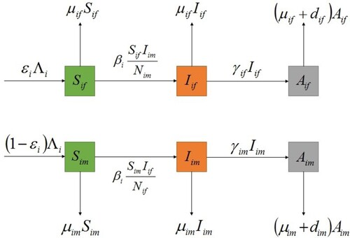
In this section, we propose a susceptible-infected-AIDS (SIA) model with standard incidence for the heterosexual transmission of HIV/AIDS with population migration between patches. A patch can be interpreted as a city, a province or a country, etc. Let n be the total number of patches. In patch i, the population is divided into six subclasses: the susceptible female, the susceptible male, the infective female (no clinical symptoms of AIDS), the infective male, the AIDS female and the AIDS male whose numbers are denoted by respectively. Susceptible individuals are transformed into infected individuals through contact with heterosexual infected individuals. The total population in patch i at time t is given by
. The flow diagram of HIV/AIDS transmission in patch i is illustrated in Figure .
We assume that susceptible individuals become infected individuals through contact with heterosexual infected individuals and they have the same transmission rate. Moreover, we assume that susceptible individuals, infected individuals and AIDS individuals of each patch have the same migration rate. Based on these assumptions, a multi-patch SIA epidemic model with standard incidence is expressed in terms of the following system of ordinary differential equations:
(1)
(1) where
,
,
. Then
.
is the total population over all patches at time t, then
. The parameters in this model are all non-negative constants. We summarize the state variables and the model parameters in Table . The migration matrix
is not required to be symmetric, namely, the migration rate from the patch i to j may not be the same as that from the patch j to i,
, where,
. Here the movement of humans between patches is governed by the Euler approach [Citation11], that is, humans change their residences when they move from one patch to another. Furthermore, it is assumed that all parameters in the model are strictly positive with the exception of the migration rates.
Figure 1. The flow diagram of HIV/AIDS transmission in patch i.
The initial conditions of system (Equation1(1)
(1) ) is given by
Table 1. State variables and parameters interpretation of system (Equation1(1)
(1) ).
Theorem 2.1
Solutions of system (Equation1(1)
(1) ) with nonnegative initial conditions uniquely exist and remain nonnegative for all time
0. Moreover, the system (Equation1
(1)
(1) ) is point dissipative.
Proof.
It is simple to verify that the vector field defined by the right-hand side of (Equation1(1)
(1) ) is locally Lipschitz on
, so there exists a unique solution of system (Equation1
(1)
(1) )
. Next, we prove the nonnegativity of the solution. By the first equation (Equation1
(1)
(1) ), we have
where
Then
Let
, then
namely
Then
Hence, we have
Similarly,
.
Let and
. The total population over all patches, denoted by
, satisfies
which implies that
. Thus the system (Equation1
(1)
(1) ) is point dissipative.
Let
since all off-diagonal entries of A and B are non-positive, it follows from the first and the forth equations of (Equation1
(1)
(1) ) that
when
for
. Thus the feasible region of (Equation1
(1)
(1) ) can be chosen as
It can be verified that X is positively invariant with respect to (Equation1
(1)
(1) ).
3. Mathematical analysis
In this section, we first study the existence and uniqueness of the disease-free equilibrium for (Equation1(1)
(1) ) and calculate the basic reproduction number
. Then, we study the stability of the disease-free equilibrium. Finally, we study the existence, uniqueness and stability of the endemic equilibrium.
3.1. Disease-free equilibrium and the basic reproduction number
To find the disease-free equilibrium of (Equation1(1)
(1) ), we consider the following linear system:
where
,
,
,
. Since all off-diagonal entries of A are non-positive and the sum of the entries in each column of A is positive, so A is a nonsingular M-matrix and
[Citation9]. Hence, linear system
has a unique positive solution
. Mathematically, if
for all i at a steady state, then by summing the third equation of (Equation1
(1)
(1) ) up from 1 to n, we have
Hence,
. This implies
for
. In the same way, linear system
has also a unique positive solution
and
for
. As a consequence, system (Equation1
(1)
(1) ) has a unique disease-free equilibrium
.
To derive the basic reproduction number for (Equation1(1)
(1) ), we use the next generation operator approach as described by Diekmann [Citation13] and van den Driessche and Watmough [Citation31]. Let
then system (Equation1
(1)
(1) ) can be written as
where
Then the new infection and transition matrices are, respectively, given by
where
and
Since
, for i = 1, 2, 3, 4, is a strictly diagonally dominant matrix, by the Gershgorin circle theorem, the real parts of its eigenvalues are positive and therefore
exists. So the inverse of V exists and equals
Thus the next generation matrix of system (Equation1
(1)
(1) ) is
By calculating
, we find the basic reproduction number
where ρ represents the spectral radius of the matrix.
The basic reproduction number for the ith patch in isolation (i.e. there is no migration between patch i and other patches) is given by
3.2. Global stability of the disease-free equilibrium
Following Theorem 2 of [Citation31], we have the following result on the local stability of .
Define
=max{
is an eigenvalue of F−V}, so
is a simple eigenvalue of F−V with a positive eigenvector [Citation28]. By Theorem 2 of van den Driessche and Watmough [Citation31], there hold two equivalences:
Theorem 3.1
The disease-free equilibrium of system (Equation1
(1)
(1) ) is locally asymptotically stable if
and unstable if
.
Proof.
To prove the local stability of disease-free equilibrium of system (Equation1
(1)
(1) ), we check the hypotheses (A1)–(A5) in [Citation31]. Hypotheses (A1)–(A4) are easily verified, while (A5) is satisfied if all eigenvalues of the
matrix
have negative real parts, where
The eigenvalues of
are the eigenvalues of F−V and
. The matrices A and B are two nonsingular M-matrices. Thus
and
have all eigenvalues with negative real parts, so
has all eigenvalues with negative real parts. Consequently, the local stability of the disease-free equilibrium depends only on eigenvalues of F−V. Thus if
, then
and
, the disease-free equilibrium
of system (Equation1
(1)
(1) ) is locally asymptotically stable.
Theorem 3.2
The disease-free equilibrium of system (Equation1
(1)
(1) ) is globally asymptotically stable if
.
Proof.
Since ,
, thus
(2)
(2) Consider the following auxiliary system:
(3)
(3) The right side has the coefficient matrix F−V. Since
if and only if
. By the Perron Frobenius theorem, all eigenvalues of the matrix F−V have negative real parts when
. Therefore it has
as
Using the comparison principle of Smith and Waltman, namely Theorem B.1[Citation28], we know that
as
. So, (Equation1
(1)
(1) ) is an asymptotically autonomous system with limit affine system
By the theory of asymptotic autonomous system of Thieme [Citation29], it is also known that
,
. So
is globally attractive when
. It follows that the disease-free equilibrium
of system (Equation1
(1)
(1) ) is globally asymptotically stable when
.
3.3. The uniform persistence of system (1)
Using the techniques of persistence theory [Citation36], we can show the uniform persistence of the disease and the existence of at least one endemic equilibrium when . Thus the basic reproduction number
is a threshold parameter of the disease dynamics. The proof below is analogous to those of Theorem 2.3 in Wang and Zhao [Citation33] and Theorem 3.7 in Gao and Ruan [Citation15].
Theorem 3.3
For system (Equation1(1)
(1) ), assume that
is irreducible, then if
, the disease is uniformly persistent, i.e. there exists a constant k>0, such that every solution
,
,
of system (Equation1
(1)
(1) ) with
,
,
,
satisfies
and (Equation1
(1)
(1) ) admits at least one endemic equilibrium.
Proof.
Let
It suffices to prove that repels uniformly the solutions of system (Equation1
(1)
(1) ) in
. Clearly,
is relatively closed in X. It is immediate that X and
are positively invariant. Theorem 2.1 implies that system (Equation1
(1)
(1) ) is point dissipative.
Denote . Obviously,
. On the other hand, we have
for any
. By the irreducibility of the migration matrix
, we know that
for all t>0. Therefore,
and
, which implies that
.
The disease-free equilibrium is the unique equilibrium in
. Let
be the stable manifold of
. We now show that
when
.
Let . Since
if and only if
, there is an
such that
for
. Choose η small enough such that
and
for
,
.
We now show that for
, where
is the usual Euclidean norm. Suppose not, then
for
and
Consider an auxiliary system
Note that
has a positive eigenvalue
associated to a positive eigenvector. By the comparison theorem, we have
The above conclusions contradict the assumptions. Since
is globally stable in
, it follows that
is an isolated invariant set and
. By Theorem 4.6 in Thieme [Citation30], system (Equation1
(1)
(1) ) is uniformly persistent with respect to
.
3.4. Uniqueness and global stability of the endemic equilibrium
In this section, if , we derive a sufficient condition that the endemic equilibrium is unique and globally asymptotically stable. Our proof utilizes the graph-theoretical approach developed in [Citation16, Citation17, Citation23].
Theorem 3.4
Assume that is irreducible, and there exist
such that
for all
, then the endemic equilibrium
of system (Equation1
(1)
(1) ) is unique and globally asymptotically stable in int(X) when
.
The proof process of Theorem 3.4, see Appendix 1.
4. Application to two patches
In the case where the patch number n is 2, (Equation1(1)
(1) ) reduces to
(4)
(4) where the parameters
and
denote, respectively, the migration rates from patches 1 to 2 and from patches 2 to 1.
If , the unique disease-free equilibrium of (Equation4
(4)
(4) ) is
where
Now
becomes
, where
where
Its characteristic equation is
we have
It is easy to see that
When the relationship between and
satisfies bc−ad + a + d−1 = 0,
.
The basic reproduction number for the ith patch in isolation (i.e. there is no migration between patch i and other patches) is given by
It is well known that
is a reproduction number of the disease in the first patch and
is a reproduction number of the disease in the second patch.
If , and there exist
such that
and
, the unique endemic equilibrium of (Equation4
(4)
(4) ) is
where
where
5. Numerical simulations
To have a more comprehensive understanding of the spread of HIV/AIDS between patches, we conduct numerical simulations for different situations to present various possible results. We introduce it from three aspects: in Section 5.1, we present time series diagrams under different conditions; in Section 5.2, we use contour plots to show the relationship between and migration rates; in Section 5.3, we make a comparison between no migration and migration.
We consider a particular case of system (Equation1(1)
(1) ) with two patches. We study the impact of population migration on the spread of HIV/AIDS epidemic with heterosexual transmission. At the same time, we also verify the theoretical analysis. We choose the data from the Beijing City and Yunnan Province, Beijing City is regarded as the first patch, Yunnan Province is regarded as the second patch. We choose 2017 as the initial time. The initial population size is given as follows:
respectively. The data is from Chinese Center for Disease Control and Prevention [Citation4], Beijing Municipal Bureau of Statistics [Citation2] and Yunnan Provincial Bureau of Statistics [Citation3]. Given that women generally live longer than men and men have higher death rates due to AIDS, we choose
, and
is selected from the range of 0.011−0.95 [Citation26]. For the transfer rates from stage
to
and from stage
to
in the two regions, we select the populations of I (the infected) and A (the AIDS) in the two regions from 2015 to 2017 from the China Center for Disease Control and prevention to calculate their average, consider that men have higher transfer rates from stage I to A than women, we choose
. For convenience, these model parameters values in numerical simulations are given in Table , with a time scale of a year.
Table 2. Model parameter values in numerical simulations.
5.1. Time series diagrams
To fully understand the spread of disease between patches, we will present time series diagrams under different conditions. For system (Equation1(1)
(1) ), we present some cases where the disease dies out or persists in each isolated patch but becomes endemic or extinct, respectively, when there are suitable migration rates between them. We simulate the changes of susceptible, infected and AIDS individuals over time in two patches in each case.
and
are the basic reproduction numbers for both patches in isolation. If
, then we call patch i a low-risk patch in isolation, while if
, then we call it a high-risk patch in isolation.
is the basic reproduction number when two patches are connected.
5.1.1. 
Assuming ,
. We fix the migration rates by letting
thus the basic reproduction numbers for both patches in isolation are
,
. This shows when there is no migration between the two patches, they are low-risk patches and the disease dies out in both patches.
If we fix the migration rates by letting and get
. This shows that the disease still dies out in both patches. Time series diagrams of different individuals in two patches are presented in Figure .
5.1.2.
Assuming ,
. We fix the migration rates by letting
thus the basic reproduction numbers for both patches in isolation are
,
. This shows when there is no migration between the two patches, they are high-risk patches and the disease becomes endemic in both patches. If we fix the migration rates by letting
and get
. This shows that the disease still becomes endemic in both patches and there exists an endemic equilibrium. Time series diagrams of different individuals in two patches are presented in Figure .
Figure 2. Time series diagrams of different individuals in two patches with , other parameters are shown in Table , and the basic reproduction number
: (a) susceptible individuals, (b) infective individuals and (c) AIDS individuals.
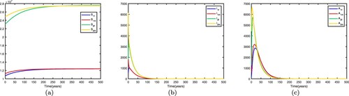
5.1.3.
Assuming ,
. We fix the migration rates by letting
that is, there is no migration between the two patches. Thus the basic reproduction numbers for both patches in isolation are
,
. This shows that the disease becomes endemic in high-risk patch 1 and dies out in low-risk patch 2. When migration occurs and migration rates are set differently, the spread of disease may be different. If we fix the migration rates by letting
thus
. Therefore, the disease-free equilibrium of (Equation1
(1)
(1) )
is globally asymptotically stable, the disease dies out in two patches, which means that patch 1 changes from a high-risk patch to a low-risk patch. In this way, migration can decrease the spread of disease. Time series diagrams of different individuals in two patches are presented in Figure .
Figure 3. Time series diagrams of different individuals in two patches with , other parameters are shown in Table , and the basic reproduction number
: (a) susceptible individuals, (b) infective individuals and (c) AIDS individuals.
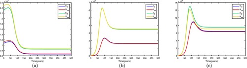
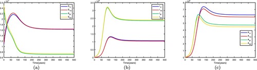
If we fix the migration rates by letting thus
. Hence, the endemic equilibrium of (Equation1
(1)
(1) )
is globally asymptotically stable, the disease becomes endemic in both patches and there exists an endemic equilibrium, which means that patch 2 changes from a low-risk patch to a high-risk patch. In this way, migration can increase the spread of disease. Time series diagrams of different individuals in two patches are presented in Figure .
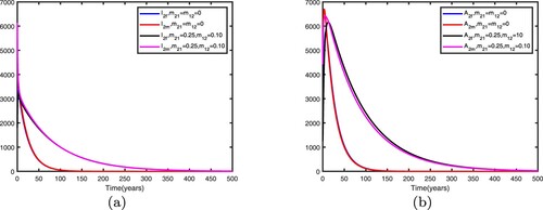
5.1.4.
Assuming ,
. We fix the migration rates by letting
that is, there is no migration between the two patches. Thus the basic reproduction numbers for both patches in isolation are
,
. This shows that the disease dies out in low-risk patch 1 and becomes endemic in high-risk patch 2. When migration occurs and migration rates are set differently, the spread of disease may be different.
If we fix the migration rates by letting thus
. Therefore, the disease-free equilibrium of (Equation1
(1)
(1) )
is globally asymptotically stable, the disease dies out in two patches, which means that patch 2 changes from a high-risk patch to a low-risk patch. In this way, migration can decrease the spread of disease. Time series diagrams of different individuals in two patches are presented in Figure . If we fix the migration rates by letting
thus
. Therefore, the disease becomes endemic in both patches and there exists an endemic equilibrium, which means that patch 1 changes from a low-risk patch to a high-risk patch. In this way, migration can increase the spread of disease. Time series diagrams of different individuals in two patches are presented in Figure .
These cases suggest that the effect of population migration on disease transmission is related to the status of the two patches in isolation. If HIV/AIDS becomes extinct in each patch when two patches are isolated, the disease remains extinct in two patches when the population migration occurs; if HIV/AIDS spreads in each patch when two patches are isolated, the disease remains persistent in two patches when the population migration occurs; if the disease disappears in one patch and spreads in the other patch when they are isolated, the disease can spread or disappear in two patches if migration rates of individuals are suitably chosen.
Figure 4. Time series diagrams of different individuals in two patches with , other parameters are shown in Table , and the basic reproduction number
: (a) susceptible individuals, (b) infective individuals and (c) AIDS individuals.
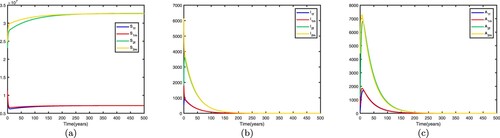
Figure 5. Time series diagrams of different individuals in two patches with , other parameters are shown in Table , and the basic reproduction number
: (a) susceptible individuals, (b) infective individuals and (c) AIDS individuals.
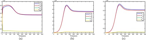
Figure 6. Time series diagrams of different individuals in two patches with , other parameters are shown in Table , and the basic reproduction number
: (a) susceptible individuals, (b) infective individuals and (c) AIDS individuals.
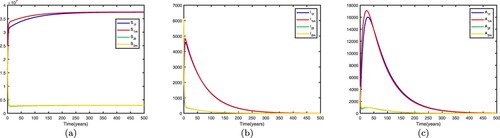
Figure 7. Time series diagrams of different individuals in two patches with , other parameters are shown in Table , and the basic reproduction number
: (a) susceptible individuals, (b) infective individuals and (c) AIDS individuals.
5.2. versus migration rates and
Sections 5.1.1 –5.1.4 show that the different migration rates between two patches may have different impacts on the spread of HIV/AIDS. To further understand the impacts of migration rates on the spread of HIV/AIDS, we use contour plots to show the relationship between and migration rates.
5.2.1.
In Figure , when the respective basic reproduction numbers of the disease for both patches in isolation are
, and no matter how migration rates
and
are set,
. Thus if HIV/AIDS becomes extinct in each patch when two patches are isolated, the disease remains extinct in two patches when population migration between two patches occurs.
5.2.2.
In Figure , when the respective basic reproduction numbers of the disease for both patches in isolation are
, and no matter how migration rates
and
are set,
. Thus if HIV/AIDS spreads in each patch when two patches are isolated, the disease remains persistent in two patches when population migration between two patches occurs.
5.2.3.
In Figure , according to Section 5.1.3, when
. Thus HIV/AIDS spreads in the first patch (Beijing City) and disappears in the second patch (Yunnan Province) when two patches are isolated. The red line denotes ‘
’, that is the relationship between
and
satisfies bc−ad + a + d−1 = 0. When the relationship between
and
is below the red line, that is bc−ad + a + d−1<0, then
, which means the disease will disappear in the two patches, otherwise it will spread.
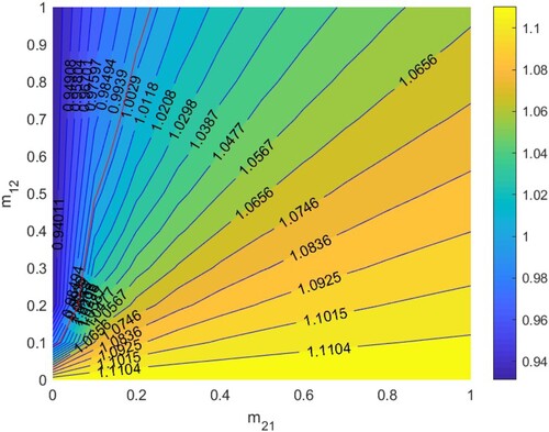
5.2.4.
In Figure , according to Section 5.1.4, when
. Thus HIV/AIDS disappears in the first patch (Beijing City) and spreads in the second patch (Yunnan Province) when two patches are isolated. The red line denotes ‘
’, that is the relationship between
and
satisfies bc−ad + a + d−1 = 0. When the relationship between
and
is above the red line, that is bc−ad + a + d−1<0, then
, which means the disease will disappear in the two patches, otherwise it will spread.
If two patches are low-risk when isolated, they are still low-risk regardless of migration. If two patches are high-risk when isolated, they are still high-risk regardless of migration. If one patch is low-risk and the other is high-risk in isolation, migration may make two patches low-risk and two patches high-risk. Therefore, when two patches are low-risk in isolation, we hardly need to control the migration rates. When one patch is low-risk and the other patch is high-risk in isolation, we can control the migration rates to make according to Figures and , so that two patches are low-risk. Otherwise, if the migration rates are not properly controlled, the low-risk patch may become high-risk patch. After that, no matter how the migration rates are controlled, it is difficult to reverse the situation, and the disease will spread in two patches.
Figure 8. The contour plot of the basic reproduction number versus migration rates
and
under parameters setting:
. Other parameters are shown in Table .
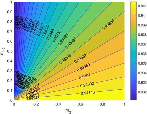
Figure 9. The contour plot of the basic reproduction number versus migration rates
and
under parameter setting:
. Other parameters are shown in Table .
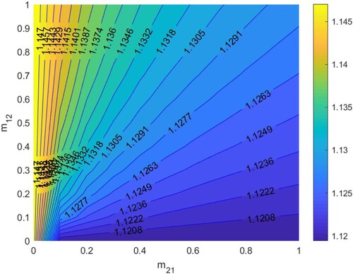
Figure 10. The contour plot of the basic reproduction number versus migration rates
and
under parameters setting:
. Other parameters are shown in Table .
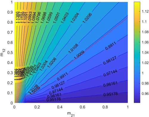
Figure 11. The contour plot of the basic reproduction number versus migration rates
and
under parameters setting:
. Other parameters are shown in Table .
5.3. Comparison between no migration and migration in two patches
We consider . When there is no migration between the two patches, i.e.
, the basic reproduction numbers for both patches in isolation are
. This shows that when there is no migration between the two patches, the disease becomes endemic in patch 1 and dies out in patch 2.
Figure 12. Comparison between no migration and migration in patch 1 with Other parameters are shown in Table : (a) infective individuals and (b) AIDS individuals.
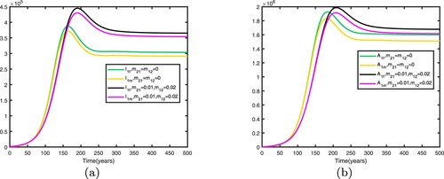
Figure 13. Comparison between no migration and migration in patch 2 with Other parameters are shown in Table : (a) infective individuals and (b) AIDS individuals.
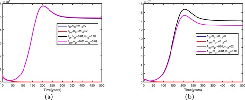
Figure 14. Comparison between no migration and migration in patch 1 with Other parameters are shown in Table : (a) infective individuals and (b) AIDS individuals.
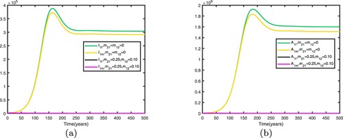
Figure 15. Comparison between no migration and migration in patch 2 with Other parameters are shown in Table : (a) infective individuals and (b) AIDS individuals.
We fix the migration rates by letting , thus
. Therefore, the disease becomes endemic in both patches and there exists an endemic equilibrium. Comparison between no migration and migration in patch 1 is presented in Figure and comparison between no migration and migration in patch 2 is presented in Figure . We fix the migration rates by letting
, thus
. Therefore, the disease dies out in two patches and there exists a disease-free equilibrium. Comparison between no migration and migration in patch 1 is presented in Figure , comparison between no migration and migration in patch 2 is presented in Figure .
It can be seen from Figures and that when migration occurs, the disease is still prevalent in patch 1, and the number of infected individuals becomes more; the disease also begin to spread in patch 2. It can be seen from Figures and that when migration occurs, the disease disappears in patch 1; the disease still disappears in patch 2.
6. Sensitivity analysis of the basic reproduction number
To analyse the effects of the parameter values on the basic reproduction number of system (Equation1
(1)
(1) ), we perform sensitivity analysis by Latin square sampling and partial rank correlation coefficient (PRCC) methods [Citation24]. We tested for significant PRCC for parameters of
. When
, PRCC is given in Table , and PRCC values of the parameters against the basic reproduction number
are shown Figure . When
, PRCCs are given in Table , and PRCC values of the parameters against the basic reproduction number
are shown in Figure . The parameters
and
of system (Equation1
(1)
(1) ) have positive and significant impact on the basic reproduction number
, which indicate that decreasing the transmission rates of sexual
and
in two patches is two effective measures to reduce the basic reproduction number
. The parameters
have negative impacts on the basic reproduction number
, of which
have more significant negative impacts on
. It means that if these transfer rates can be strictly controlled,
will decrease, that is, if the number of infected individuals can be controlled, the disease will gradually disappear. We have shown that the impact of migration rates
and
on the basic reproduction number
is always one positive and one negative. In Figure , when
,
has a positive impact and
has a negative impact. This is also shown in Figures and of the contour plots. However, in Figure , when
,
has a negative impact and
has a positive impact. This is also shown in Figures and of the contour plots. Therefore, we should effectively control the migration rates according to the actual situation of the two patches, so as to reduce
and make the disease disappear gradually. From the perspective of the research process, the most effective measure to control and prevent HIV/AIDS spread is to reduce contact with infected individuals, thereby reducing the parameter values of
and
. From the perspective of control,
can be reduced by increasing publicity, education and using condoms, etc. In Figure , it is shown that decreasing transmission rates can reduce the spread of HIV/AIDS in two patches. Hence, to control the spread of HIV/AIDS, the intervention measure must be taken.
7. Conclusion
Cosner et al. [Citation12] and Sattenspiel et al. [Citation27] introduced two models of human movement, including Euler movement model and Lagrange movement model. Citron et al. [Citation11] further introduced the two models and examples were given to illustrate how to combine the two models with the research problems. Therefore, Euler movement and Lagrange movement are usually considered for individual movement.
Figure 16. Value of correlation coefficient for outcome when
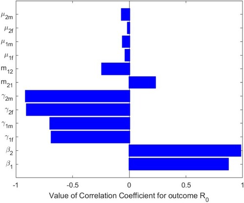
Figure 17. Value of correlation coefficient for outcome when
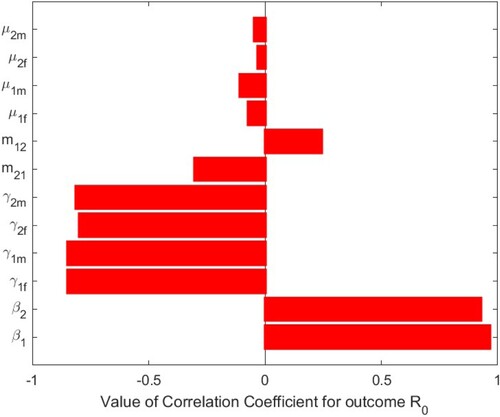
Figure 18. Influence of different transmission rate parameters on HIV/AIDS transmission in two patches with . Other parameters are shown in Table : (a) infective individuals in patch 1, (b) AIDS individuals in patch 1, (c) infective individuals in patch 2 and (d) AIDS individuals in patch 2.
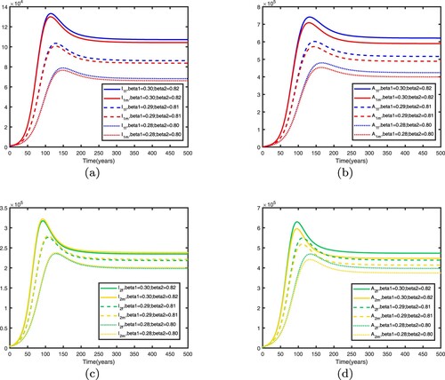
Table 3. The PRCC of the parameters in system (Equation1(1)
(1) ) when
.
Table 4. The PRCC of the parameters in system (Equation1(1)
(1) ) when
.
In this paper, we considered the movement of individuals as the form of Euler movement. And we have proposed an HIV/AIDS epidemic model with heterosexual transmission in a patchy environment to study the dynamics of disease transmission under the influence of population migration among patches. A patch can be interpreted as a city, a province or a country, etc. We have shown that implies that the disease-free equilibrium is unique and globally asymptotically stable and
implies that the disease is uniformly persistent if migration matrix
is irreducible. If
is irreducible and there exist
such that
for all
, the endemic equilibrium
is unique and globally asymptotically stable. We have selected two patches for numerical simulations. We have chosen the data from the Beijing City and Yunnan Province, Beijing City is regarded as the first patch, Yunnan Province is regarded as the second patch. Population migration may increase the spread of disease, turning a low-risk patch into a high-risk patch, or it may reduce the spread of disease, turning a high-risk patch into a low-risk patch. The effect of population migration on disease transmission is related to the status of the two patches in isolation. If HIV/AIDS becomes extinct in each patch when two patches are isolated, the disease remains extinct in two patches when the population migration occurs; if HIV/AIDS spreads in each patch when two patches are isolated, the disease remains persistent in two patches when the population migration occurs; if the disease disappears in one patch and spreads in the other patch when they are isolated, the disease can spread or disappear in two patches if migration rates of individuals are suitably chosen. We have shown that the impacts of migration rates
and
on the basic reproduction number
is always one positive and one negative. When
,
has a positive impact and
has a negative impact; when
,
has a negative impact and
has a positive impact. When two patches are low-risk in isolation, we hardly need to control the migration rates. When one patch is low-risk and the other patch is high-risk in isolation, we can control the migration rates to make
according to Figures –, so that two patches are low-risk. Otherwise, if the migration rates are not properly controlled, the low-risk patch may become high-risk patch. After that, no matter how the migration rates are controlled, it is difficult to reverse the situation, and the disease will spread in two patches. Therefore, we should effectively control the migration rates according to the actual situation of the two patches, so as to reduce
and make the disease reduce gradually. In addition, Figure has shown that reducing contact with infected individuals, i.e. reducing the parameter values of
and
is also a key measure to reduce the spread of the disease. The model established in this paper is helpful to understand the spread of HIV/AIDS among regions when population migration occurs. In addition, the model can also be used in other regions. These studies enrich the research on patches.
Acknowledgments
The authors would like to thank the referees for their helpful suggestions that improved the presentation of this manuscript.
Disclosure statement
No potential conflict of interest was reported by the author(s).
Additional information
Funding
References
- World Health Organization, 10 facts about HIV/AIDS. Available at http://www.who.int/news-room/facts-in-pictures/detail/hiv-aids.
- Beijing Municipal Bureau of Statistics. Available at http://tjj.beijing.gov.cn/.
- Yunnan Provincial Bureau of Statistics. Available at http://stats.yn.gov.cn/.
- Chinese Center for Disease Control and Prevention. Available at https://ncaids.chinacdc.cn/
- Julien Arino and P. Van Den Driessche, A multi-city epidemic model, Math. Popul. Stud. 10 (2003), pp. 175–193.
- Julien Arino and Pauline Van Den Driessche, The basic reproduction number in a multi-city compartmental epidemic model, in Positive Systems, Springer, 2003, pp. 135–142.
- Julien Arino and P. Van Den Driessche, Disease spread in metapopulations, Fields Inst. Commun. 48 (2006), pp. 1–13.
- Nicolas Bacaër, Xamxinur Abdurahman, and Jianli Ye, Modeling the HIV/AIDS epidemic among injecting drug users and sex workers in kunming, China, Bull. Math. Biol. 68 (2006), pp. 525–550.
- Abraham Berman and Robert J. Plemmons, Nonnegative Matrices in the Mathematical Sciences, SIAM, 1994.
- Liming Cai, Xuezhi Li, Mini Ghosh, and Baozhu Guo, Stability analysis of an HIV/AIDS epidemic model with treatment, J. Comput. Appl. Math. 229 (2009), pp. 313–323.
- Daniel T. Citron, Carlos A. Guerra, Andrew J. Dolgert, Sean L. Wu, John M. Henry, and David L.Smith, Comparing metapopulation dynamics of infectious diseases under different models of human movement, Proc. Natl. Acad. Sci. 118 (2021), Article ID e2007488118.
- Chris Cosner, John C. Beier, Robert Stephen Cantrell, D. Impoinvil, Lev Kapitanski, Matthew DavidPotts, A. Troyo, and Shigui Ruan, The effects of human movement on the persistence of vector-borne diseases, J. Theor. Biol. 258 (2009), pp. 550–560.
- Odo Diekmann, Johan A.J. Heesterbeek, and Johan Andre PeterMetz, On the definition and the computation of the basic reproduction ratio R0 in models for infectious diseases in heterogeneous populations, J. Math. Biol. 28 (1990), pp. 365–382.
- Daozhou Gao, Travel frequency and infectious diseases, SIAM J. Appl. Math. 79 (2019), pp. 1581–1606.
- Daozhou Gao and Shigui Ruan, An SIS patch model with variable transmission coefficients, Math. Biosci. 232 (2011), pp. 110–115.
- Hongbin Guo, Michael Y. Li, and Zhisheng Shuai, Global stability of the endemic equilibrium of multigroup SIR epidemic models, Can. Appl. Math. Q. 14 (2006), pp. 259–284.
- Hongbin Guo, Michael Li, and Zhisheng Shuai, A graph-theoretic approach to the method of global Lyapunov functions, Proc. Am. Math. Soc. 136 (2008), pp. 2793–2802.
- Yu Jin and Wendi Wang, The effect of population dispersal on the spread of a disease, J. Math. Anal. Appl. 308 (2005), pp. 343–364.
- Kate E. Jones, Nikkita G. Patel, Marc A. Levy, Adam Storeygard, Deborah Balk, John L. Gittleman, and Peter Daszak, Global trends in emerging infectious diseases, Nature 451 (2008), pp. 990–993.
- Hossein Kheiri and Mohsen Jafari, Stability analysis of a fractional order model for the HIV/AIDS epidemic in a patchy environment, J. Comput. Appl. Math. 346 (2019), pp. 323–339.
- J.P. LaSalle, The Stability of Dynamical Systems, Regional Conference Ser, Applied Mathematics, SIAM, Philadelphia, 1976.
- Michael Li and Zhisheng Shuai, Global stability of an epidemic model in a patchy environment, Can. Appl. Math. Q. 17 (2009), pp. 175–187.
- Michael Y. Li and Zhisheng Shuai, Global-stability problem for coupled systems of differential equations on networks, J. Differ. Equ. 248 (2010), pp. 1–20.
- Simeone Marino, Ian B. Hogue, Christian J. Ray, and Denise E. Kirschner, A methodology for performing global uncertainty and sensitivity analysis in systems biology, J. Theor. Biol. 254 (2008), pp. 178–196.
- Robert K. Mccormack and Linda J.S. Allen, Multi-patch deterministic and stochastic models for wildlife diseases, J. Biol. Dyn. 1 (2007), pp. 63–85.
- Z. Mukandavire, W. Garira, and C. Chiyaka, Asymptotic properties of an HIV/AIDS model with a time delay, J. Math. Anal. Appl. 330 (2007), pp. 916–933.
- Lisa Sattenspiel and Klaus Dietz, A structured epidemic model incorporating geographic mobility among regions, Math. Biosci. 128 (1995), pp. 71–91.
- Hal L. Smith and Paul Waltman, The Theory of the Chemostat: Dynamics of Microbial Competition, Cambridge University Press, 1995.
- Horst R. Thieme, Convergence results and a Poincaré–Bendixson trichotomy for asymptotically autonomous differential equations, J. Math. Biol. 30 (1992), pp. 755–763.
- Horst R. Thieme, Persistence under relaxed point-dissipativity (with application to an endemic model), SIAM J. Math. Anal. 24 (1993), pp. 407–435.
- Pauline Van den Driessche and James Watmough, Reproduction numbers and sub-threshold endemic equilibria for compartmental models of disease transmission, Math. Biosci. 180 (2002), pp. 29–48.
- Wendi Wang and G. Mulone, Threshold of disease transmission in a patch environment, J. Math. Anal. Appl. 285 (2003), pp. 321–335.
- Wendi Wang and Xiao-Qiang Zhao, An epidemic model in a patchy environment, Math. Biosci. 190 (2004), pp. 97–112.
- Xinxin Wang, Shengqiang Liu, Lin Wang, and Weiwei Zhang, An epidemic patchy model with entry–exit screening, Bull. Math. Biol. 77 (2015), pp. 1237–1255.
- Juping Zhang, Chris Cosner, and Huaiping Zhu, Two-patch model for the spread of West Nile virus, Bull. Math. Biol. 80 (2018), pp. 840–863.
- Xiao-Qiang Zhao, Dynamical Systems in Population Biology Vol. 16, Springer, 2003.
- Hongyong Zhao, Peng Wu, and Shigui Ruan, Dynamic analysis and optimal control of a three-age-class HIV/AIDS epidemic model in China, Discrete Continuous Dyn. Syst. Ser. B 25 (2020), pp. 3491–3521.
Appendix
Appendix 1.
Proof of Theorem 3.4
Proof.
By Theorem 3.3, the existence of an endemic equilibrium is ensured. We prove that
is globally asymptotically stable in int(X).
First, we prove that if there exist such that
for
,
is the only endemic equilibrium. We consider the following system:
(A1)
(A1) From the first two equations of (EquationA1
(A1)
(A1) ), we have
or in the form of matrix
where
,
and
. Therefore, we have
, where
. Since
, hence
, where
. Since all off-diagonal entries of
is non-positive and the sum of the entries in each column of
is positive, so
is a nonsingular M-matrix and
, hence
. In the same way, we have
, where
and
. Therefore, we have
, where
. Since
, hence
, where
. We obtain
.
We write the third and sixth equations of (EquationA1(A1)
(A1) ) in matrix form respectively, i.e.
and
, where
. Since all off-diagonal entries of
and
are non-positive and the sum of the entries in each column of
and
is positive, so they are two nonsingular M-matrices,
. Therefore, linear system
has a unique positive solution
, linear system
has a unique positive solution
,
, and
.
Then we prove that the endemic equilibrium of system (Equation1
(1)
(1) ) is globally asymptotically stable in int(X) when
.
Define by
From equilibrium equations of (Equation1
(1)
(1) ), we obtain
Note that
for x>0 and equality holds if and only if x = 1. Calculating the time derivative of
along solutions of system (Equation1
(1)
(1) ), we have
where
Consider two weight matrices
with entry
and
with entry
, and denote the corresponding weighted digraphs as
and
. Let
,
. Then
Set
then
Therefore, V is a Lyapunov function for system (Equation1
(1)
(1) ). Since
is irreducible, from Theorem 2.1 in [Citation23], we know that
and
for all i, and thus
implies that
for all i. From the third and sixth equations of (Equation1
(1)
(1) ), we obtain
which implies that
for all i. From the first and fourth equations of (Equation1
(1)
(1) ), we obtain
which implies that
for all i, thus
. The largest (and only) invariant set on which
is the singleton
. Therefore, by LaSalle Invariance Principle [Citation21],
is globally asymptotically stable when
.