
 ?Mathematical formulae have been encoded as MathML and are displayed in this HTML version using MathJax in order to improve their display. Uncheck the box to turn MathJax off. This feature requires Javascript. Click on a formula to zoom.
Abstract
Ehrlichia chaffeensis is a tick-borne disease transmitted by ticks to dogs. Few studies have mathematical modelled such tick-borne disease in dogs, and none have developed models that incorporate different ticks' developmental stages (discrete variable) as well as the duration of infection (continuous variable). In this study, we develop and analyze a model that considers these two structural variables using integrated semigroups theory. We address the well-posedness of the model and investigate the existence of steady states. The model exhibits a disease-free equilibrium and an endemic equilibrium. We calculate the reproduction number (). We establish a necessary and sufficient condition for the bifurcation of an endemic equilibrium. Specifically, we demonstrate that a bifurcation, either backward or forward, can occur at
, leading to the existence, or not, of an endemic equilibrium even when
. Finally, numerical simulations are employed to illustrate these theoretical findings.
1. Introduction
Ehrlichiosis are tick-borne diseases caused by obligate intracellular rickettsia bacteria in the genera Ehrlichia [Citation1–5]. These bacteria are classified within the group of the α-proteobacteria, order Rickettsiales, family Anaplasmataceae, genus Ehrlichia [Citation3,Citation6]. This genus consists of obligate intracellular Gram-negative bacteria [Citation1,Citation4,Citation6] that mainly infect leukocytes (such as monocytes, macrophages, granulocytes and neutrophils), and endothelial cells in mammals, and salivary glands, intestinal epithelium, and hemolymph cells of ticks [Citation1,Citation7–12]. The genus Ehrlichia comprises of six recognized tick-transmitted species: E. canis, E. muris, E. chaffeensis, E. ewingii, E. minasensis, and E. ruminantium [Citation3,Citation11], and in recent times, other Ehrlichia species have been reported [Citation7,Citation8,Citation11]. Going by our current knowledge, a large number of Ehrlichia species might not have been described [Citation11].
The reservoir hosts for Ehrlichia species include numerous wild animals, as well as some domesticated species and livestock [Citation6]. Some of these Ehrlichia species affect animals including pets such as cats and dogs [Citation6,Citation13], and a limited number have been know to infect humans [Citation2,Citation4,Citation6,Citation13–16]. Specifically, Ehrlichia canis, E. chaffeensis, E. ewingii, E. muris, and E. ruminantium are members of the genus Ehrlichia known to naturally infect various mammalian hosts such as cats, dogs, ruminants, and mice, and are responsible for emerging zoonoses in humans [Citation7,Citation8,Citation10,Citation17].
Ehrlichia are tick-borne diseases transmitted by ticks in the family Ixodidae. Rhipicephalus sanguineus (brown dog tick) and Ixodes ricinus are vectors for Ehrlichia canis [Citation5,Citation6]. E. canis can also be transmitted by Amblyomma cajennense, and experimentally by Dermacentor variabilis (American dog tick) [Citation6]. In North America A. americanum (Lone Star tick) is the primary vector for both E. chaffeensis and E. ewingii [Citation4,Citation6,Citation18,Citation19]. ‘Outside North America, E. chaffeensis has been found in ticks in the genera Amblyomma, Haemaphysalis, Dermacentor, and Ixodes in Asia, in R. sanguineus in Cameroon, and in A. parvum in Argentina’ [Citation6]. Haemaphysalis flava and Ixodes persulcatus complex ticks transmits E. muris [Citation6]. E. ruminantium is the only known Ehrlichia species that infects cattle and it is found on the continent of Africa and a couple of Caribbean islands [Citation8].
Ticks life-cycle span between 2-to-3 years depending on the species [Citation20,Citation21]. They go through four life stages namely egg, six-legged larva, eight-legged nymph, and adult. To survive each life stage after hatching from eggs, the ticks must take a blood meal from a host; but, most ticks will die if they are unable to find a host [Citation20]. Ticks feed once on a host, then fall off and develop into the next stage. This feeding pattern creates pathways for diseases to be transmitted from hosts to hosts [Citation22]. Ixodes scapularis (black-legged tick) life cycle generally lasts two years, while the life cycle of Amblyomma americanum (the lone star tick) is around three years long [Citation21]. Some species like Rhipicephalus sanguineus (the brown dog tick) whose primary host is the domestic dog, prefer to feed on the same host during all its life stages [Citation20,Citation22]. Since R. sanguineus are endophilic, they are found inside houses and dog kennels [Citation22].
Dogs are susceptible to infection with multiple Ehrlichia spp., including E. chaffeensis, E. ewingii, and E. canis [Citation2,Citation12,Citation19,Citation23,Citation24]. In 2019, over 200,000 dogs tested positive for antibodies against Ehrlichia spp. within the United States out of 7,056,709 dogs tested, while over 1000 dogs tested positive out of 168,216 dogs tested in Canada [Citation25]. According to Gettings et al. [Citation25] the distribution of infected dogs follows the distribution of the related tick vectors. For instance, Amblyomma americanum is commonly found on dogs and people in the southeastern and southcentral United States [Citation2]. In Beall et al. [Citation2] the overall seroprevalence of E. canis, E. chaffeensis, and E. ewingii across the United States in 2012 was 0.8%, 2.8%, and 5.1%, respectively. The highest E. canis seroprevalence of 2.3% was found in Arkansas, Louisiana, Oklahoma, Tennessee, and Texas. E. chaffeensis seroreactivity was 6.6% in Arkansas, Kansas, Missouri, and Oklahoma (the central region), and 4.6% in Georgia, Maryland, North Carolina, South Carolina, Tennessee and Virginia (the southeast region). Seroreactivity of E. ewingii was highest in the central region with 14.6% value while the southeast region had a seroreactivity value of 5.9%.
Ehrlichia in dogs was discovered in the 1970s when military dogs were returning from the Vietnam war. They found this disease to be extremely severe in German Shepards, Doberman Pinschers, Belgium Malinois, and Siberian Huskies. Several studies including experimental researches and serological surveys have been carried out to understand Ehrlichiosis transmission in canine including Ehrlichia Chaffeensis [Citation1,Citation15,Citation26–28]. We only found two quantitative studies modelling Ehrlichiosis in human [Citation29,Citation30]. Thus, in this study, we developed a mathematical model for Amblyomma americanum in the Great Plains and dogs infected with Ehrlichia Chaffeensis with the aim of understanding the quantitative properties of the model including the asymptotic dynamics of the disease in dogs across the Plains.
The rest of the paper is organized as follows: Section 2 gives the description of the model including the interactions between the ticks and dogs; Section 3 describes the results of the study. These results include the existence and uniqueness of solutions, the disease invasion process, and the bifurcation analysis. More precisely, we show that, depending on the sign of a constant – referred to as the bifurcation parameter – which depends on model's parameters, a bifurcation occurs at
that is either a forward or backward bifurcation. In a forward bifurcation, which occurs when
, there exists a unique endemic equilibrium if and only if
. However, in a backward bifurcation, which occurs when
, no endemic equilibrium exists for
small enough; a unique endemic equilibrium exists if
while multiple equilibria exist when
close enough to 1. Finally in Section 4 we numerically illustrate such bifurcation results.
2. Model formulation
The transmission model of Ehrlichia Chaffeensis incorporates two subgroups: dogs and ticks. At any time t, the dog population is divided into susceptible , infected
, and chronically infected
, recovered
. Here, the variable a represents the time since infection. Thus, the total number of dogs at time t is quantified by
The ticks population is structured into several stages: eggs (E), larva (L), nymph (N), and adult (A). We denote by
the set of ticks stages. Let
be the number of susceptible ticks of stage
at time t. We also denote by
the number of infected ticks of stage
at time t and which are infected since time a. The model proposed assumes that there are no infected eggs. Therefore the total number of ticks of stage
at time t is given by
(1)
(1) The dogs-ticks infection life cycle is shown in Figure .
Figure 1. Flow chart of the model.
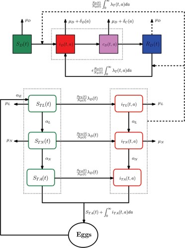
Dogs' population dynamic. At any time t, infected ticks (which are infected since time a) induce an infection within the dogs' population through the force of infection , such that
(2)
(2) where
denotes the infectivity of infected ticks. Therefore, newly infected dogs are given by
and
, where ϵ is constant parameter accounting for the relative disease transmission to previously recovered dogs. Note that ϵ can be considered age-dependent (
) with no more difficulties in the analysis proposed here. Thus, the dogs population dynamic is then described by the below system
(3)
(3) In the above model, susceptible dogs are recruited at rate
and all dogs die naturally at rate
. Infected and chronically infected dogs have a disease-induced mortality rate
and
. Infected dogs progress to a chronic infection at rate
. Finally, only non-chronic infections are assumed to recover from the infection at rate γ.
Ticks' population dynamic. At time t, infected dogs (chronic or not) induce an infection within the ticks population through the force of infection , such that
where
denotes the infectivity of infected and chronically infected dogs a-time post infection. Therefore, newly infected ticks of stage
are given by
. The ticks population dynamic is then described by the system below
(4)
(4) with
. In the above system of the ticks dynamic, the eggs' production rate at time t is
, where
is the number of eggs produced by adult ticks
, and the parameter K is the eggs' carrying capacity. Parameters
,s are ticks progression rates from the eggs' to adult' stage. The death rate of ticks at each k-stage is
. The notations of all variables and parameters are summarized in Table .
Table 1. State variables and parameters used for simulations.
3. Main results
This section is devoted to the main results of this paper. Overall, our results are based on the following assumption on the parameters of system (Equation3(3)
(3) )–(Equation4
(4)
(4) ). More precisely, we assume that
Assumption 3.1
| (1) | The recruitment rate | ||||
| (2) | Parameters | ||||
| (3) | The initial condition is such that | ||||
3.1. Existence and uniqueness of nonnegative solution
In this section, we state the results concerning the existence of a globally defined nonnegative solution to system (Equation3(3)
(3) )–(Equation4
(4)
(4) ).
In order to state our main results, we will rewrite the system in a more appropriate equivalent form. To do this, denote by and
,
the canonical basis of
and
, respectively. Thus, we can consider the states variables in a vector form by setting for every
and
Moreover, we define the vector
of transmission rates with components
and
, i.e.
and define the vector
. Let
be ticks stage progression matrix from the larval stage to the adult stage, i.e.
(5)
(5) Therefore, using the notation
to denotes the inner product in
and
and setting for all
(6)
(6) Model (Equation3
(3)
(3) )–(Equation4
(4)
(4) ) takes the following form
(7)
(7) and
(8)
(8) subject to the initial condition
,
,
,
,
,
, and
. The following result then concerns the existence and uniqueness of nonnegative solutions to (Equation7
(7)
(7) )–(Equation8
(8)
(8) ).
Theorem 3.2
Let Assumption 3.1 be satisfied. Then there exists a unique continuous globally defined integrated solution to (Equation7(7)
(7) )–(Equation8
(8)
(8) ). Moreover, if we set
(9)
(9) then the solution satisfies, for all
and
,
and
Moreover, the total population of Dogs,
, at time t is the unique solution to
(10)
(10)
Proof.
The existence and positiveness of solutions of system (Equation3(3)
(3) )–(Equation4
(4)
(4) ) can be addressed using an integrated semigroup approach and Volterra integral formulation. More precisely, a similar approach as in [Citation37] can be applied for detailed proof of Theorem 3.2. However, here we give a brief sketch of such an approach. For all
, let us set
where
is the space
Such a Banach space
is endow with the usual product norm
.
Let :
the linear operator defined by
and
as well as the map
such that
Observe that the nonlinear map
is not well defined on
due to the term
and is then not locally Lipschitz continuous. Furthermore, for any
, let us introduce the space
where
is the operator defined by
We can now define the nonlinear operator
by
. Therefore, system (Equation7
(7)
(7) )–(Equation8
(8)
(8) ) can be rewritten as the following non-densely defined abstract Cauchy problem:
(11)
(11) We then address the existence and uniqueness of bounded solutions to (Equation11
(11)
(11) ) in a manner similar to the approach in [Citation37].
3.2. Disease invasion process
System (Equation7(7)
(7) )–(Equation8
(8)
(8) ) exhibits two disease-free equilibria. More precisely, in an infection-free environment, we have a disease-free equilibrium either in the presence of dogs and ticks or only in the presence of dogs. But, only the former is interesting within this context because the disease is transmitted from dogs to ticks and vice versa. Such an equilibrium is named after the disease-free equilibrium of system (Equation3
(3)
(3) )–(Equation4
(4)
(4) ). Let us introduce the following threshold parameter
(12)
(12) The parameter
accounts for the ticks' reproduction number and is such that,
represents the fraction of eggs that progress to the larval stage,
is the fraction of larval that progress to the nymphal stage,
is the fraction of nymph that progress to the adult stage,
is the life expectancy of adult ticks and
is the ticks egg laying rate. Furthermore, when
, the disease-free equilibrium of system (Equation3
(3)
(3) )–(Equation4
(4)
(4) ) is given by
(13)
(13) where
(14)
(14) In the last equality, the correspondence
,
, and
is used to facilitate the notations. See Section 6 for a detailed computation of
.
Next, we introduce the following threshold
(15)
(15) where
quantifies the transmission capability from dogs to ticks and
the transmission capability from ticks to dogs. More precisely, we have
and
(16)
(16) where
denotes the vectorial capacity of ticks population of stage k and is explicitly given by
(17)
(17) with
(18)
(18) The map
(resp.
) describes the probability to still be infected (resp. chronically infected) a-time post-infection. Based on the above notations, we now state the invasion dynamics in terms of the threshold
defined in (Equation15
(15)
(15) ).
Theorem 3.3
Let Assumption 3.1 be satisfied. Assume in addition that the ticks' reproduction number satisfies . Then the following properties hold true:
| (i) | If | ||||
| (ii) | If | ||||
The proof of Theorem 3.3 is given in Section 7.
3.3. Existence of an endemic equilibrium and bifurcation
In this section, we state our main result concerning necessary and sufficient conditions for the existence of an endemic equilibrium to system (Equation7(7)
(7) )–(Equation8
(8)
(8) ) and forward (resp. backward) bifurcation at
. Denote by
an endemic equilibrium to system (Equation7
(7)
(7) )–(Equation8
(8)
(8) ) that is a time-independent solution to system (Equation7
(7)
(7) )–(Equation8
(8)
(8) ).
(19)
(19) with
(20)
(20) such that
,
,
,
,
, and
. By means of scaling and a suitable change of variables, we prove in Section 8 that the existence of an endemic equilibrium
can be reduced to the existence of a positive solution of one equation with one unknown. More precisely, we prove that there exists an endemic equilibrium
if and only if there exists K>0 satisfying
with
The maps
,
, and
are given by
and the function
is defined by
with
(resp.
) is the vectorial (k's ticks stage vectorial) capacity given in (Equation16
(16)
(16) ) (resp. in (Equation17
(17)
(17) )). Recall that in the above sum, we have used the notations
,
, and
with
. Furthermore, if we consider the bifurcation parameter
then we have the following results whose proof is given in Section 8.
Theorem 3.4
Let Assumption 3.1 be satisfied. Assume in addition that the ticks' reproduction number satisfies . Then the following properties hold true
| (i) | If | ||||
| (ii) | If | ||||
4. Numerical simulations
In this section, we present numerical simulations to illustrate the forward and backward bifurcation results of Model (Equation3(3)
(3) )–(Equation4
(4)
(4) ). These simulations were conducted using finite volume numerical schemes implemented with the R software (http://www.r-project.org/). The values of the parameters used are given in Table . In all the figures, we have used the initial conditions
,
,
,
,
,
,
,
,
,
,
. Given the parameter values in Table , the ticks' reproduction number
.
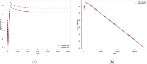
A forward bifurcation occurs at (Theorem 3.4), which means that whenever
, then the disease-free equilibrium
is locally asymptotically stable (Theorem 3.3) and no endemic equilibrium exists. Asymptotically, the disease go extinct (Figure (b), where
). However, if
, then
is unstable (Theorem 3.3) and an endemic equilibrium exists if
(Theorem 3.4). The disease is asymptotically persistent and the solution converges to the endemic equilibrium (Figure (a), where
and
).
Figure 2. Forward bifurcation diagram with convergence either to (a) the endemic equilibrium when ; (b) the disease-free equilibrium when
. Here
,
,
,
,
, and
are fixed. The probability of infection
is considered constant with: (a)
and (b)
. The other parameters are given by Table .
A backward bifurcation occurs at . This means that whenever
, the disease-free equilibrium is unstable and there exists a unique endemic equilibrium. In such a situation, the solutions converge asymptotically to this endemic equilibrium (Figures (a)), where
). By contrast to the forward bifurcation (Figures and (a)), when
and
there exists an endemic equilibrium (Theorem 3.4). Furthermore, there exists a threshold
such that (i) for
, there is no endemic equilibrium and the solutions converge to the disease-free equilibrium (Figures (b) and (b), where
) and (ii) for
, there exist an endemic equilibrium such that, depending on the initial condition, the solution can converge to this endemic equilibrium (Figures (c) and (b), where
).
Figure 3. Backward bifurcation diagram with convergence either to (a) the endemic equilibrium when ; (b) the disease-free equilibrium when
; (c) the endemic equilibrium when
. Here
,
,
,
,
, and
are fixed. The probability of infection
is considered constant with: (a)
, (b)
, and (c)
. The other parameters are given by Table .
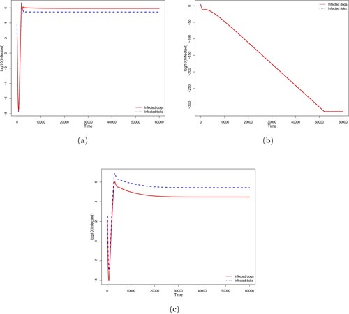
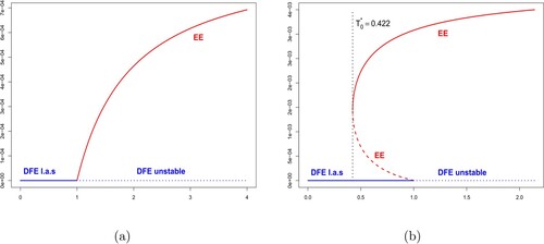
Figure 4. Forward and backward bifurcation diagram. (a) Forward bifurcation diagram with where all the parameters are the same as in Figure . (b) Backward bifurcation diagram with
and the parameters are the same as in Figure . Note that
does not depend on the parameter
.
5. Discussion and conclusions
5.1. Discussion
In this work, we have developed a novel partial differential equation (PDE) model that extends classical epidemiological models proposed for tick-borne diseases (see [Citation29,Citation30]). The model proposed here incorporates the ability to accurately account for the different ticks' developmental stages (discrete variable) as well as the variations in infectiousness over the course of infection (continuous variable). In our study, we established the mathematical well-posedness of the model using the integrated semigroups theory. However, the presence of singularity in the force of infection whenever the total dogs' population is zero introduces a complication to the analysis. Note that this is a mathematical construct, since without dogs the model would not hold nor make sense.
We derived an explicit formula for the reproduction number , extending the classical formula. We identified two possible behaviours around
. The first scenario involves a forward bifurcation, indicating that an epidemic can only occur if
. In the second scenario, a backward bifurcation is observed, where an epidemic can arise if
, provided that
is sufficiently close to 1. These findings have significant epidemiological implications, especially in an endemic region where controlling the epidemic is of importance. In the forward bifurcation case, simply reducing the reproduction number
below 1 is sufficient to halt the epidemic. However, in the backward bifurcation scenario, the number must be reduced below a second threshold, denoted as
.
The epidemiological implication of the backward bifurcation phenomenon is that the classical requirement of having the basic reproduction number () less than one is no longer sufficient to ensure effective disease eradication or elimination [Citation38]. This implies that disease can invade to a relatively high endemic level once the reproduction number
is more than one; decreasing
below one do not necessarily make the disease disappear, see Figure (b) and Figure in [Citation38]. Backward bifurcation has been shown to occur in several vector-borne disease models [Citation37,Citation39–45]. For instance Garba et al. [Citation44] showed for a dengue model the possibility of backward bifurcation where a locally stable disease-free equilibrium coexists with a locally stable endemic equilibrium. Also, the age-structure malaria and Chikungunya models in [Citation37,Citation39,Citation42,Citation43] were shown to exhibit backward bifurcation when
is less than one. This phenomenon is equally possible in the absence of any age-structure [Citation39,Citation42,Citation43]. Backward bifurcation in these vector-borne disease models is induced by disease induced mortality. Furthermore, backward bifurcation can equally be induced by several other factors like vaccination [Citation46–49], exogenous re-infection which are known to occur in tuberculosis models [Citation50–52], and cross-immunity for instance in a two strain influenza transmission model [Citation53]. Other epidemiological mechanism like differential susceptibility in risk-structured models could also cause backward bifurcation in disease transmission models [Citation38]. We should note that the age-structured Ehrlichia chaffeensis model (Equation3
(3)
(3) )–(Equation4
(4)
(4) ) include disease induce death (
and
) in the dog population and hence the source of the backward bifurcation.
5.2. Conclusion
In conclusion, we have developed a novel partial differential equation model of Ehrlichia chaffeensis transmission dynamics in dogs. The model incorporates the different developmental life stages of ticks (discrete variable) as well as the duration of infection (continuous variable). The following results were obtained from our theoretical analysis and numerical simulations:
The developed model is well-posed;
The model always exhibits a disease-free equilibrium along with an endemic equilibrium;
The model has a reproduction number, denoted as
;
A necessary and sufficient condition for the bifurcation of an endemic equilibrium was established using semigroup approach;
A bifurcation (forward or backward), can occur at
6. The disease-free equilibrium of (3)–(4)
The dynamic of ticks in the absence of infection is governed by the following system of equations
(21)
(21) with initial condition
,
,
, and
. It is easy to see that
is invariant with respect to the ordinary differential equation so that if
then the larval, nymphal, and adult stages exponentially goes to 0. From this, we have that a necessary condition for the ticks to persist is
. Moreover, by straightforward computations, we find that (Equation21
(21)
(21) ) has a unique positive stationary solution if and only if the ticks reproduction number
defined by (Equation12
(12)
(12) ) satisfies
. By straightforward computations, we have that the equilibrium of system (Equation21
(21)
(21) ) is given by
(22)
(22) Note that in accordance with the compact formulation (Equation7
(7)
(7) )–(Equation8
(8)
(8) ), the above expressions of
and
, with
, can be rewritten as
(23)
(23) and
(24)
(24) and using the correspondence
,
, and
.
7. Threshold and proof of Theorem 3.3
In order to obtain the threshold of (Equation7(7)
(7) )–(Equation8
(8)
(8) ) that determine disease invasion dynamics in a completely susceptible population of ticks and dogs, we consider the linearized equation to (Equation7
(7)
(7) )–(Equation8
(8)
(8) ) at the disease-free equilibrium
. More precisely, we linearize the infective compartments of (Equation7
(7)
(7) )–(Equation8
(8)
(8) ) around
to obtain the following system
(25)
(25) and
(26)
(26) whose initial conditions satisfy
and
. In order to define the threshold and study the local asymptotic stability of the disease-free equilibrium, we will make use of the semigroup approach by reformulating (Equation25
(25)
(25) ) and (Equation26
(26)
(26) ) as an abstract Cauchy problem. For this purpose, we consider the Banach spaces
,
,
and
. Let
and
be the linear operators defined by
with
Let
with
Let
be the bounded linear operator defined by
(27)
(27) where we have set for each
and each
Hence, setting for all t>0
and
the system (Equation25
(25)
(25) )–(Equation26
(26)
(26) ) can be rewritten as the following abstract Cauchy problem
(28)
(28) In order to define the threshold that determines the local asymptotic stability of the disease-free equilibrium, we need first to prove the following lemma. Before proceeding, let us set
,
,
, and
.
Lemma 7.1
Let Assumption 3.1 be satisfied. Then the following properties hold true
| (i) |
| ||||
| (ii) | The spectral bound | ||||
Proof.
In order to obtain the conclusion of the lemma, we first prove that is resolvent positive. To do this, let us note that if
then
and
so that the resolvent of
is obtained by determining the resolvent of
and
. By standard computations, we have for each
and
(30)
(30) (where
is defined in (Equation9
(9)
(9) )) while for each
and
we have
(31)
(31) Next, recalling the definition of
and
respectively in (Equation5
(5)
(5) ) and (Equation6
(6)
(6) ) it follows that if
(32)
(32) then
. Next, recalling from [Citation54,Citation55] if
is resolvent positive then
(33)
(33) and we infer from (Equation30
(30)
(30) ) to (Equation33
(33)
(33) ) that
. The proof is completed.
Thanks to Lemma 7.1 and the positiveness of the bounded linear operator (i.e. it maps
into
), one can use the theory developed in [Citation56] to define a threshold which determines the sign of
i.e. the spectral bound of
given by
More precisely, we set
(34)
(34) where
is the spectral radius of the bounded linear operator
. The following lemma will allow us to obtain the relationship between the sign of
and the growth bound of the C
-semigroup generated by
i.e. the part of
in
. Note that the latter threshold
does not exhibit explicitly the parameters of the model but this will be resolved after proving the local stability properties.
Lemma 7.2
Let Assumption 3.1 be satisfied. Then and
have the same sign. Moreover, we have the following properties
| (i) |
| ||||
| (ii) |
| ||||
Proof.
We first note that is an AL-space [Citation56, Theorem 3.14] with positive cone
that is normal and generating (see [Citation56]) so that
(35)
(35) with
the growth bound of the C
-semigroup generated by
. The first assertion of the lemma is a direct application of [Citation56, Theorem 3.5]. Next, we prove properties (i) and (ii). Since
and
(see [Citation57]) it follows that
and
. This proves (i) and the equality
. Next, note that
is compact since
is a finite-dimensional space. Therefore, we infer from [Citation58, Theorem 1.2] that
and the proof is completed.
Lemma 7.3
Let Assumption 3.1 be satisfied. Assume in addition that the ticks' reproduction number satisfies . Then the disease-free equilibrium is locally asymptotically stable if
and unstable if
.
Proof.
If then by Lemma 7.3 we have
resulting to the local asymptotic stability of the disease-free. If
then
and since
it follows that
. Therefore, using [Citation58, Theorem 3.2.] one knows that
has an isolated positive eigenvalue. Thus we refer to [Citation57, Proposition 5.7.4]) that the disease-free equilibrium is unstable.
The threshold defined in (Equation34
(34)
(34) ) is somehow abstract and does not allow the interpretation of the stability of the disease-free to be made in terms of the parameters of the model. Therefore, we will give in the following and equivalent threshold which incorporate explicitly the parameters of the model. To this end, we first make a remark that allows us to simplify the determination of
. Let us set
, and
. Next, we observe that
is finite-dimensional and
so that the spectral bound of
coincides with the spectral bound of
. The advantage of considering
is that we can obtain the spectral radius by solving an eigenvalue problem of a matrix.
Proposition 7.4
Let Assumption 3.1 be satisfied. Assume in addition that the ticks' reproduction number satisfies and set
(36)
(36) Then
and
have the same sign.
Proof.
We first give the explicit form of the linear operator . Let
be given with
and
. Then using the resolvent formula of
and
respectively in (Equation30
(30)
(30) ) and (Equation31
(31)
(31) ) we obtain
(37)
(37) and
(38)
(38) Hence using the explicit form of
in (Equation27
(27)
(27) ) it comes
(39)
(39) with
so that the spectral radius of
is given by the spectral radius of the linear operator
given by
Since
is a positive linear operator of finite-dimensional spaces, its spectral radius
is an eigenvalue. Moreover, let
be a non zero vector such that
. Then we have the following system of equations
(40)
(40) from where we obtain the equality
(41)
(41) Hence, plugging (Equation41
(41)
(41) ) into the first equation of (Equation40
(40)
(40) ) gives
Thus, setting
and recalling that
,
, and
we obtain by identification
so that
(42)
(42) From the above computations, we see that
is the null vector if and only if
. Therefore, the spectral radius of
satisfies
(43)
(43) with
Next, observe that
defined in (Equation15
(15)
(15) ) is also given by
. Moreover, by similar computations, one obtains that the non-zero eigenvalues of
satisfy
(44)
(44) To prove that
and
have the same sign, we will make use of (Equation43
(43)
(43) ) and (Equation44
(44)
(44) ). Indeed if
then (Equation43
(43)
(43) ) implies that
. If
then (Equation44
(44)
(44) ) becomes
with
so that the non-zero solution of (Equation44
(44)
(44) ) have modulus less than one. This proves that
whenever
. To complete the proof, we observe that if
then (Equation43
(43)
(43) ) implies that
. Similarly if
then
.
8. Proof of Theorem 3.4
In order to determine the endemic equilibrium of the model (Equation7(7)
(7) )–(Equation8
(8)
(8) ), we proceed in several steps. In the first step, we give an equivalent system to (Equation45
(45)
(45) ), the second step is concerned with the solvability of (Equation46
(46)
(46) ), and the last step concerns the bifurcation properties. In this section, we will always suppose that Assumption 3.1 is satisfied and
. Let us note that using the notation (Equation18
(18)
(18) ) together with Theorem 3.2, one knows that an endemic equilibrium
defined in (Equation19
(19)
(19) ) satisfies
(45)
(45) and
(46)
(46) On the stationary states of ticks: Let us first prove the following lemma which describes the stationary states of the eggs.
Lemma 8.1
The total number of eggs remains unchanged at the endemic and the disease-free equilibrium i.e. . Moreover, we always have
(47)
(47)
Proof.
Note that, using the third equation of (Equation45(45)
(45) ) we have
(48)
(48) Next, integrating the second equation of (Equation45
(45)
(45) ) it follows that
(49)
(49) Thus, by combining (Equation48
(48)
(48) ) and (Equation49
(49)
(49) ) we obtain
(50)
(50) Therefore, plugging (Equation50
(50)
(50) ) in the first equation of (Equation53
(53)
(53) ) we obtain the following equality
(51)
(51) or equivalently
(52)
(52) The right-hand side of (Equation52
(52)
(52) ) is a decreasing function of
so that the unique solution to (Equation51
(51)
(51) ) is
. The equality (Equation47
(47)
(47) ) now follows from (Equation50
(50)
(50) ).
Thanks to Lemma 8.1 the system of equations (Equation45(45)
(45) ) is equivalent to
(53)
(53) Note that for each nonnegative constant
the matrix
(where
is the identity operator on
) is invertible with inverse
satisfying
(54)
(54) and where the correspondence
,
, and
is used. Therefore, using (Equation53
(53)
(53) ) together with (Equation54
(54)
(54) ), for
, it follows that
(55)
(55) with
and
. Thus, recalling the expression of
in (Equation24
(24)
(24) ) we obtain
(56)
(56) and the system of equations (Equation53
(53)
(53) ) becomes equivalent to
(57a)
(57a)
(57b)
(57b)
(57c)
(57c) From the above comments, it follows that
and
are entirely determined by the variables
and
.
On the stationary states of dogs: In order to obtain an equivalent formulation to (Equation46(46)
(46) ) we introduce the new variables
(58)
(58) Next, we set
(59)
(59) and
(60)
(60) With these new variables, system (Equation46
(46)
(46) ) becomes
(61)
(61) which is equivalent to
(62)
(62) Next, we show the relationship between
and
defined respectively in (Equation57c
(57c)
(57c) ) and (Equation59
(59)
(59) ). To do so, we integrate (Equation57b
(57b)
(57b) ) to obtain
(63)
(63) and by using the expression of
defined in (Equation57a
(57a)
(57a) ) we obtain the following more explicit formula
(64)
(64) with
the k's stage vectorial capacity defined in (Equation17
(17)
(17) ).
In the following, we determine the equations for the variables ,
,
,
and
defined in (Equation60
(60)
(60) ). To this end, recalling that
, we use successively the equation of
in (Equation62
(62)
(62) ) to obtain
(65a)
(65a)
(65b)
(65b)
(65c)
(65c)
(65d)
(65d)
(65e)
(65e)
(65f)
(65f)
Note that, plugging (Equation65d(65d)
(65d) ) into (Equation65a
(65a)
(65a) ) gives the following equality
(66)
(66) Let us now define the function
(67)
(67) and observe that the vectorial capacity
is given by
(68)
(68) so that
(69)
(69) In the following, we rewrite our system of equations by using the variable
(70)
(70) To do so, we first observe that (Equation66
(66)
(66) ) and (Equation64
(64)
(64) ) take respectively the following form
(71)
(71) while (Equation65a
(65a)
(65a) ) is now given by
(72a)
(72a)
(72b)
(72b)
(72c)
(72c)
(72d)
(72d)
(72e)
(72e)
(72f)
(72f) Hence, using the first equation of (Equation62
(62)
(62) ) together with (Equation72e
(72e)
(72e) ), and (Equation72f
(72f)
(72f) ) we obtain the following necessary conditions
(73)
(73) Furthermore, the second, third and fourth equation of (Equation62
(62)
(62) ) together with (Equation71
(71)
(71) ), (Equation72c
(72c)
(72c) ) and (Equation72d
(72d)
(72d) ) provide
(74a)
(74a)
(74b)
(74b)
(74c)
(74c) Moreover, from the equality
and (Equation70
(70)
(70) ) it comes that for K>0 we must have the following equality
(75)
(75) Recalling that we have the necessary condition
, we consider the following equation
with
(76)
(76) and
(77)
(77)
Lemma 8.2
There exists an endemic equilibrium to (Equation7(7)
(7) )–(Equation8
(8)
(8) ) if and only if there exists K>0 such that
.
Proof.
The necessity of the lemma follows from the preceding arguments. Next, we prove the sufficiency. To this end, assume that there exists K>0 such that . Let
be given by the right-hand side of (Equation73
(73)
(73) ). Let
and
be given respectively by the right-hand side of (Equation74a
(74a)
(74a) ) and (Equation74c
(74c)
(74c) ). Observe that with these definitions we have
(78)
(78) so that setting
(79)
(79) it comes from (Equation76
(76)
(76) )
(80)
(80) Note that setting
,
, with f defined in (Equation67
(67)
(67) ), and multiplying (Equation80
(80)
(80) ) by K it follows that
(81)
(81) Therefore, our definition of
and
respectively in (Equation74a
(74a)
(74a) ) and (Equation74c
(74c)
(74c) ) together with (Equation81
(81)
(81) ) give us
(82)
(82) Moreover, using (Equation81
(81)
(81) ) one also note that our definition of
in (Equation73
(73)
(73) ) leads to
(83)
(83) Next, we observe that the
-equation in (Equation82
(82)
(82) ) is equivalent to
(84)
(84) Note that from the above formulas of
and
in (Equation82
(82)
(82) ) we have the following identities
(85)
(85) from where we can rewrite (Equation83
(83)
(83) ), (Equation84
(84)
(84) ) and the
-equation in (Equation82
(82)
(82) ) as follow
(86)
(86) Next, observe that
(87)
(87) so that by integrating (Equation87
(87)
(87) ) from 0 to
we obtain
and by using (Equation85
(85)
(85) ) it follows that
(88)
(88) Next, multiply (Equation89
(89)
(89) ) by
and use the first equation of (Equation86
(86)
(86) ) to obtain
(89)
(89) Hence, summing (Equation89
(89)
(89) ) and the second equation of (Equation86
(86)
(86) ) it follows that
(90)
(90) that is
(91)
(91) Finally, we infer from the
-equation of (Equation86
(86)
(86) ), the equality (Equation91
(91)
(91) ) together with our definition of
, and
that (Equation62
(62)
(62) ) is satisfied. The proof is completed by using the fact that we have set
with
and f given by (Equation67
(67)
(67) ).
Thanks to Lemma 8.2, the existence of positive equilibrium to (Equation7(7)
(7) )–(Equation8
(8)
(8) ) is subjected to the existence of K>0 such that
(92)
(92) where
is given by (Equation76
(76)
(76) ) and (Equation77
(77)
(77) ). Before studying the existence of solution to (Equation92
(92)
(92) ), we first observe that from (Equation73
(73)
(73) ), (Equation74a
(74a)
(74a) ) and (Equation77
(77)
(77) ) we have
(93)
(93) We also note that for each
we have
(94)
(94) with
Therefore, using the equality
it follows from (Equation93
(93)
(93) ) and (Equation76
(76)
(76) ) that
(95)
(95) It is now clear from (Equation95
(95)
(95) ) that for each
there exists
such that
. In particular, if
then there exists
such that
leading to the existence of an endemic equilibrium.
On the forward and backward bifurcations: In the following, we deal with the existence of forward and backward bifurcation at . Roughly speaking, we have to prove that there exists a positive map
defined in some right neighbourhood (forward bifurcation) or left neighbourhood (backward bifurcation) of
such that
and
. Since
, one can prove the existence of forward and backward bifurcations using implicit function theorem which is reduced here to the study of
. This motivates the following lemma.
Lemma 8.3
The following property is satisfied
(96)
(96) and
Proof.
Since for each
the first equality of the lemma follows. To compute
, it is enough to take the derivative of
with respect to K at K = 0. To do so let us first note that by using (Equation76
(76)
(76) ) we have
Recalling that
,
,
and taking the derivative of
with respect to K at K = 0 it follows that
By straightforward computations, we obtain from (Equation73
(73)
(73) ) and (Equation77
(77)
(77) ) that
and
To complete the proof it remains to compute
and
. We first compute
. To this end, we compute the derivative of
from (Equation74a
(74a)
(74a) ) with respect to K and set K = 0 to obtain
To compute
recall that
so that setting
we obtain
Therefore, computing the derivative of
one obtains
and since
it follows that
that is
(97)
(97) The proof is completed.
Thanks to Lemma 8.3 one knows that if then by the implicit function theorem there exists
and a smooth map
such that
(98)
(98) Thus, up to reduce ξ, it follows that the sign of
on
is given by the sign of
at
. Differentiating (Equation98
(98)
(98) ) with respect to
and using Lemma 8.3 we obtain
so that
If
If
Disclosure statement
No potential conflict of interest was reported by the author(s).
Additional information
Funding
References
- AV Barrantes-González, AE Jiménez-Rocha, JJ Romero-Zuñiga, et al. Understanding ehrlichia canis infections in dogs of costa rica: hematological findings and indicative clinical signs. Open J Vet Med. 2016;06(11):163–175. doi: 10.4236/ojvm.2016.611020
- MJ Beall, AR Alleman, EB Breitschwerdt, et al. Seroprevalence of ehrlichia canis, ehrlichia chaffeensis and ehrlichia ewingii in dogs in North America. Parasit Vectors. 2012;5(1):1–11. doi: 10.1186/1756-3305-5-29
- JS Dumler, AF Barbet, C Bekker, et al. Reorganization of genera in the families rickettsiaceae and anaplasmataceae in the order rickettsiales: unification of some species of ehrlichia with anaplasma, cowdria with ehrlichia and ehrlichia with neorickettsia, descriptions of six new species combinations and designation of ehrlichia equi and'hge agent'as subjective synonyms of ehrlichia phagocytophila. Int J Syst Evol Microbiol. 2001;51(6):2145–2165. doi: 10.1099/00207713-51-6-2145
- AD Nair, C Cheng, DC Jaworski, et al. Ehrlichia chaffeensis infection in the reservoir host (white-tailed deer) and in an incidental host (dog) is impacted by its prior growth in macrophage and tick cell environments. PLoS ONE. 2014;9(10):e109056. doi: 10.1371/journal.pone.0109056
- A Procajło, E Skupień, M Bladowski, et al. Monocytic ehrlichiosis in dogs. Pol J Vet Sci 14(3) (2011), pp. 515–520. doi:10.2478/v10181-011-0077-9
- CM Ehrlichiosis, CH Fever, TC Pancytopenia, et al. Ehrlichiosis and anaplasmosis: Zoonotic species. 2013. The Center for Food Security & Public Health, Iowa State University. Accessed on August 7 2022. https://www.cfsph.iastate.edu/Factsheets/pdfs/ehrlichiosis.pdf
- DM Aguiar, TF Ziliani, X Zhang, et al. A novel ehrlichia genotype strain distinguished by the trp36 gene naturally infects cattle in brazil and causes clinical manifestations associated with ehrlichiosis. Ticks Tick Borne Dis. 2014;5(5):537–544. doi: 10.1016/j.ttbdis.2014.03.010
- BA Allsopp. Natural history of ehrlichia ruminantium. Vet Parasitol. 2010;167(2-4):123–135. doi: 10.1016/j.vetpar.2009.09.014
- P Brouqui, K Matsumoto. Bacteriology and phylogeny of anaplasmataceae. Rickettsial Dis. 2007;191–210.
- LA Cohn. Ehrlichiosis and related infections. Vet Clin Small Anim Pract. 2003;33(4):863–884. doi: 10.1016/S0195-5616(03)00031-7
- L Fargnoli, C Fernandez, LD Monje. Novel ehrlichia strain infecting cattle tick amblyomma neumanni, Argentina, 2018. Emerging Infect Dis. 2020;26(5):1027–1030. doi: 10.3201/eid2605.190940
- M Groves, G Dennis, H Amyx, et al. Transmission of ehrlichia canis to dogs by ticks (rhipicephalus sanguineus). Am J Vet Res. 1975;36(7):937–940.
- MN Saleh, KE Allen, MW Lineberry, et al. Ticks infesting dogs and cats in north america: biology, geographic distribution, and pathogen transmission. Vet Parasitol. 2021;294:109392. doi: 10.1016/j.vetpar.2021.109392
- K Mahachi, E Kontowicz, B Anderson, et al. Predominant risk factors for tick-borne co-infections in hunting dogs from the USA. Parasit Vectors. 2020;13(1):1–12. doi: 10.1186/s13071-020-04118-x
- RFDC Vieira, TSWJ Vieira, DDAG Nascimento, et al. Serological survey of ehrlichia species in dogs, horses and humans: zoonotic scenery in a rural settlement from southern brazil. Rev Inst De Med Trop São Paulo. 2013;55(5):335–340. doi: 10.1590/S0036-46652013000500007
- CB Yancey, BC Hegarty, BA Qurollo, et al. Regional seroreactivity and vector-borne disease co-exposures in dogs in the united states from 2004–2010: utility of canine surveillance. Vector-Borne Zoonotic Dis. 2014;14(10):724–732. doi: 10.1089/vbz.2014.1592
- CD Paddock, JE Childs. Ehrlichia chaffeensis: a prototypical emerging pathogen. Clin Microbiol Rev. 2003;16(1):37–64. doi: 10.1128/CMR.16.1.37-64.2003
- BE Anderson, KG Sims, JG Olson, et al. Amblyomma americanum: a potential vector of human ehrlichiosis. Am J Trop Med Hyg. 1993;49(2):239–244. doi: 10.4269/ajtmh.1993.49.239
- O Anziani, S Ewing, R Barker. Experimental transmission of a granulocytic form of the tribe ehrlichieae by dermacentor variabilis and amblyomma americanum to dogs. Am J Vet Res. 1990;51(6):929–931.
- Centers for Disease Control and Prevention (CDC). How ticks spread disease. [accessed 2023 Aug 7]. Available from: https://www.cdc.gov/ticks/life_cycle_and_hosts.html.
- E Guo, FB Agusto. Baptism of fire: modeling the effects of prescribed fire on lyme disease. Can J Infect Dis Med Microbiol. 2022;2012.
- J van der Krogt. Ehrlichia canis infections on the island of curaçao an overview of the clinical picture and current diagnostics & therapies. 2010. Accessed August 7 2023. https://studenttheses.uu.nl/bitstream/handle/20.500.12932/4426/Ehrlichia%20canis%20infections%20on%20the%20island%20of%20Curacao%20by%20J.S.%20van%20der%20Krogt.pdf?sequence=1
- S Ewing, J Dawson, A Kocan, et al. Experimental transmission of ehrlichia chaffeensis (rickettsiales: ehrlichieae) among white-tailed deer by amblyomma americanum (acari: ixodidae). J Med Entomol. 1995;32(3):368–374. doi: 10.1093/jmedent/32.3.368
- SE Little, TP O'Connor, J Hempstead, et al. Ehrlichia ewingii infection and exposure rates in dogs from the southcentral united states. Vet Parasitol. 2010;172(3-4):355–360. doi: 10.1016/j.vetpar.2010.05.006
- JR Gettings, SC Self, CS McMahan, et al. Local and regional temporal trends (2013–2019) of canine ehrlichia spp. seroprevalence in the usa. Parasit Vectors. 2020;13(1):1–11. doi: 10.1186/s13071-020-04022-4
- MU Aziz, S Hussain, B Song, et al. Ehrlichiosis in dogs: A comprehensive review about the pathogen and its vectors with emphasis on South and East Asian countries. Vet Sci. 2023;10(1):21. doi: 10.3390/vetsci10010021
- BA Qurollo, J Buch, R Chandrashekar, et al. Clinicopathological findings in 41 dogs (2008-2018) naturally infected with ehrlichia ewingii. J Vet Intern Med. 2019;33(2):618–629. doi: 10.1111/jvim.2019.33.issue-2
- BA Qurollo, R Chandrashekar, BC Hegarty, et al. A serological survey of tick-borne pathogens in dogs in north america and the Caribbean as assessed by anaplasma phagocytophilum, a. platys, ehrlichia canis, e. chaffeensis, e. ewingii, and borrelia burgdorferi species-specific peptides. Infect Ecol Epidemiol. 2014;4(1):24699.
- H Gaff, L Gross, E Schaefer . Results from a mathematical model for human monocytic ehrlichiosis. Clin Microbiol Infect. 2009;15:15–16. doi: 10.1111/j.1469-0691.2008.02131.x
- HD Gaff, LJ Gross. Modeling tick-borne disease: a metapopulation model. Bull Math Biol. 2007;69(1):265 288 doi: 10.1007/s11538-006-9125-5
- North Shore Animal League. Prevent a litter – spay and neuter your pets. [accessed 2022 Aug 7]. Available from: https://www.animalleague.org/wp-content/uploads/2017/06/dogs-multiply-pyramid.pdf.
- A Burke. How long do dogs live?. [accessed 2022 Aug 7]. Available from: https://www.akc.org/expert-advice/health/how-long-do-dogs-live/.
- Mar Vista Animal Medical Center. Ehrlichia infection (canine). 2020 [accessed 2022 Aug 7]. Available from: https://www.marvistavet.com/ehrlichia-infection-canine.pml.
- K Williams. BSc, DVM, CCRP; Ryan Llera, BSc, DVM; Ernest Ward, DVM. Ehrlichiosis in dogs. [accessed 2022 Aug 7]. Available from: https://vcahospitals.com/know-your-pet/ehrlichiosis-in-dogs.
- C Wheeler. The life cycle of a tick. [accessed 2022 Aug 7]. Available from: https://study.com/learn/lesson/tick-life-cycle-reproduction-eggs.html.
- GH Antoinette Ludwig, HS Ginsberg, NH Ogden. A dynamic population model to investigate effects of climate and climate-independent factors on the lifecycle of amblyomma americanum. J Med Entomol 53(1) (2015), pp. 99–115.
- Q Richard, M Choisy, T Lefèvre, et al. Human-vector malaria transmission model structured by age, time since infection and waning immunity. Nonlinear Anal: Real World Appl. 2022;63:103393. doi: 10.1016/j.nonrwa.2021.103393
- AB Gumel. Causes of backward bifurcations in some epidemiological models. J Math Anal Appl. 2012;395(1):355–365. doi: 10.1016/j.jmaa.2012.04.077
- F.B. Agusto, S. Easley, K. Freeman, et al. Mathematical model of three age-structured transmission dynamics of chikungunya virus. Comput Math Methods Med. 2016;2016:1–31. doi: 10.1155/2016/4320514
- KW Blayneh, AB Gumel, S Lenhart, et al. Backward bifurcation and optimal control in transmission dynamics of West Nile virus. Bull Math Biol. 2010;72(4):1006–1028. doi: 10.1007/s11538-009-9480-0
- J Dushoff, W Huang, C Castillo-Chavez. Backwards bifurcations and catastrophe in simple models of fatal diseases. J Math Biol. 1998;36(3):227–248. doi: 10.1007/s002850050099
- F Forouzannia, A Gumel. Dynamics of an age-structured two-strain model for malaria transmission. Appl Math Comput. 2015;250:860–886.
- F Forouzannia, A Gumel. Mathematical analysis of an age-structured model for malaria transmission dynamics. Math Biosci. 2014;247:80–94. doi: 10.1016/j.mbs.2013.10.011
- SM Garba, AB Gumel, MA Bakar. Backward bifurcations in dengue transmission dynamics. Math Biosci. 2008;215(1):11–25. doi: 10.1016/j.mbs.2008.05.002
- Z Mukandavire, AB Gumel, W Garira, et al. Mathematical analysis of a model for HIV-malaria co-infection. Mathematical Biosciences and Engineering 6(2) (2009), pp. 333–362. doi:10.3934/mbe.2009.6.333
- FB Agusto, AB Gumel. Theoretical assessment of avian influenza vaccine. DCDS Ser B. 2010;13(1):1–25. doi: 10.3934/dcdsb.2010.13.1
- F Brauer. Backward bifurcations in simple vaccination models. J Math Anal Appl. 2004;298(2):418–431. doi: 10.1016/j.jmaa.2004.05.045
- EH Elbasha, AB Gumel. Theoretical assessment of public health impact of imperfect prophylactic hiv-1 vaccines with therapeutic benefits. Bull Math Biol. 2006;68(3):577–614. doi: 10.1007/s11538-005-9057-5
- O Sharomi, C Podder, A Gumel, et al. Role of incidence function in vaccine-induced backward bifurcation in some hiv models. Math Biosci. 2007;210(2):436–463. doi: 10.1016/j.mbs.2007.05.012
- C Castillo-Chavez, B Song. Dynamical models of tuberculosis and their applications. Math Biosci Eng. 2004;1(2):361–404. doi: 10.3934/mbe.2004.1.361
- Z Feng, C Castillo-Chavez, AF Capurro. A model for tuberculosis with exogenous reinfection. Theor Popul Biol. 2000;57(3):235–247. doi: 10.1006/tpbi.2000.1451
- O Sharomi, C Podder, A Gumel, et al. Mathematical analysis of the transmission dynamics of hiv/tb coinfection in the presence of treatment. Math Biosci Eng. 2008;5(1):145.174 doi: 10.3934/mbe.2008.5.145
- SM Garba, MA Safi, AB Gumel. Cross-immunity-induced backward bifurcation for a model of transmission dynamics of two strains of influenza. Nonlinear Anal Real World Appl. 2013;14(3):1384–1403. doi: 10.1016/j.nonrwa.2012.10.003
- W Arendt. Resolvent positive operators. Proc Lond Math Soc. 1987;s3-54(2):321–349. doi: 10.1112/plms/s3-54.2.321
- RD Nussbaum. Positive operators and elliptic eigenvalue problems. Math Z. 1984;186(2):247–264.
- HR Thieme. Spectral bound and reproduction number for infinite-dimensional population structure and time heterogeneity. SIAM J Appl Math. 2009;70(1):188–211. doi: 10.1137/080732870
- P Magal, S Ruan. Theory and applications of abstract semilinear Cauchy problems. Volume 201 of Applied Mathematical Sciences. Cham: Springer International Publishing; 2018.
- A Ducrot, Z Liu, P Magal. Essential growth rate for bounded linear perturbation of non-densely defined Cauchy problems. J Math Anal Appl. 2008;341(1):501–518. doi: 10.1016/j.jmaa.2007.09.074