Three-dimensional trees for virtual globes

Abstract

One of the problems in virtual globes technologies is the real-time representation of vegetal species. In forest or garden representations, the low detailed plants produce a lack of realism. Efficient techniques are required to achieve accurate interactive visualisation due to the great number of polygons the vegetal species have. This article presents a multi-resolution model based on a geometric representation of vegetal species that allows the application to perform the progressive transmission of the model, that is, the transmission of a simple representation followed by successive refinements of it. It has a hardware-oriented design in order to obtain interactive frame rates. The geometric data of the objects are stored in the graphics processing unit and, moreover, the change from one approximation to another is obtained by performing mathematical calculations in this graphics hardware. The multi-resolution model presented here enables instancing: as many vegetal species as desired can be rendered with different levels of detail, while all of them are accessing the same geometric data. This model has been used to build a real-time representation of a not imaginary scenario.

Keywords:

• virtual globes
• real-time rendering
• vegetal species
• level of detail
• graphics hardware
• progressive transmission

1. Introduction

Virtual globes are presented as three-dimensional (3D) software models, which are capable of modelling the Earth or other environments of the universe (Bailey and Chen 2011). The software releases of freely downloadable virtual globes have sparked an enormous public interest (Paraskevas 2011). One of the reasons of their popularity is probably the easy way this software is freely available. One example is Google Earth™. In a virtual globe, one moment the user may be viewing Earth from a distance and the next moment, the user may zoom in to a hill valley or to street level in a city. The freedom of exploration and the ability to visualise incredible amounts of data give virtual globes their appeal.

Virtual globes render so massive quantities of terrain and imagery. In fact, Google Earth 6 (2012) includes 3D trees modelled for several areas around the world. Google has also worked to generate larger groups of trees and forests in non-urban areas. Nevertheless, due to the geometric complexity of the trees, such amount of data must be managed with specialised techniques, which are an active area of research (Cozzi and Ring 2011). This paper focuses on the interactive rendering of gardens or forests. The lack of realism is due to the poor quality of the vegetal species representations because the vast number of polygons that forms these objects makes it necessary to use techniques that reduce their geometry. This problem becomes almost impossible to solve when the scene to be rendered in real time is an ecosystem.

Multi-resolution modelling is a well-known technique that deals with the problem of the generation, representation and manipulation of geometric objects at several levels of detail (Ribelles et al. 2002). Another application of this technique is the progressive reconstruction of images or 3D objects in order to achieve real-time viewing (To, Lau, and Green 1999). Some works (Deng et al. 2010; Gumbau et al. 2011) present geometric multi-resolution models that have been specially designed for vegetal species. They have to solve several problems in order to generate an interactive visualisation. The first problem involves the large amount of information that must be managed in a multi-resolution model, that is, the original geometry of the vegetal species and its approaches. Secondly, there is the excessive time spent on the extraction of a particular Level of Detail (LoD). This extraction process was usually performed in the central processing unit (CPU) and, in order to render this geometry, it was transferred through the bus from the CPU to the graphics processing unit (GPU). One possible solution to these problems has been to take advantage of the development of the graphics hardware. The GPU can currently process information and store it, thereby avoiding the bottleneck due to the data traffic from the CPU.

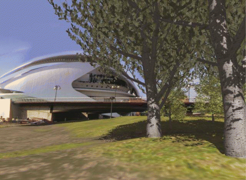
This paper presents a geometry-based multi-resolution model that adapts the LoD of the vegetal species in real time. The main advantage of this LoD model is that all geometry data are stored in the GPU, and the extraction of the appropriate LoD is also performed in this graphics hardware using some simple mathematical formulae. Thus, the extraction and rendering time become almost negligible. Moreover, this multi-resolution model represents ecosystems efficiently because of its easy implementation of instancing techniques. This LoD model has been used to build a real-time representation of a real scenario, the gardens around the Palau of the Arts, in the city of the Arts and Science in Valencia, Spain (Figure 1).

Figure 1. A close-up view of a virtual representation of the scenario surrounding the Palau of the Arts, in the city of the Arts and Science, Valencia, Spain. The vegetal species are represented using the presented multi-resolution model.

After reviewing in Section 2, the most important works published in recent years on the field of real-time visualisation of vegetal species, an explanation of the methodology of the model is given in Sections 3 and 4. Then, the details of its data structures are analysed in Section 5. The pre-process of the data and the multi-resolution model are explained and reviewed in Sections 6 and 7. The extraction and rendering processes are analysed in Section 8. Section 9 analyses the simplicity of the instantiation process and how the progressive transmission is performed by this model is detailed in Section 10. Finally, Section 11 provides the results of the modelling technique, and Section 12 provides the conclusions and discussions on the future work.

2. Related work

In virtual globes technologies, 3D models can be constructed and defined independently of the virtual globe software, such as Google Earth™ application. These 3D models have their own coordinate space, and they can be modelled using applications such as SketchUp™, 3D Studio Max, Softimage XSI or Maya (Paraskevas 2011). However, when a 3D model is imported into Google Earth™, it is translated, rotated and scaled to fit into the Google Earth™ coordinate system. The interactive representation of vegetal species in an outdoor scene can be classified into two basic groups: image-based and geometry-based techniques.

Image-based modelling replaces the geometry of the object by an image textured on polygons, blending transparency and colour. This technique offers important advantages such as its simplicity and easy implementation. Moreover, the rendering time is independent of the geometric complexity of the objects. The main drawbacks, however, are the large amount of memory required to store the images and the lack of realism when the camera is close to the object. This solution is usually based on billboards, volumetric textures or billboard clouds (Meyer, Neyret, and Poulin 2001; Decaudin and Neyret 2004, 2009; Reche, Martin, and Drettakis 2004; Behrendt et al. 2005; Lacewell et al. 2006; Linz et al. 2006; García et al. 2007; SpeedTree 2012).

Geometry-based models are mainly classified depending on the primitive used to represent them: polygons, lines and/or points. The approaches based on points and lines adapt the density and the size of these primitives depending on the scene requirements. If the density of the sample is not adequate, some holes and problems of aliasing can be detected. Stamminger and Drettakis (2001) and Mantler and Fuhrmann (2003) propose algorithms based only on points. Their representations consist in clouds of points that change to triangles when the camera is close to the objects. Wand et al. (2001) generate the scene using of triangular primitives and a dynamically chosen set of random surface sample points. Deussen et al. (2002) visualise ecosystems by combining triangles, points and lines. In run-time, and according to the projected size of each object, it is decided whether the model should be visualised using triangles, or whether it is better to use the point-and-line-based approach. Dachsbacher, Vogelgsang, and Stamminger (2003) use triangles at close-up distances, replacing them by points as the camera zooms out. Triangles are the most widely used primitive in the case of polygonal representation. The works reported in Rebollo et al. (2007), Deng et al. (2010), Gumbau et al. (2011) and Remolar et al. (2012), represent vegetal species by isolated polygons formed by the union of two triangles in a quad. Some of them can represent a view-dependent resolution, that is, different levels of detail coexisting in the same representation.

Moreover, some works have presented a solution in order to avoid the high data traffic between the CPU and the GPU, which is necessary to update the LoD of the objects. This is the case of Rebollo et al. (2007), Gumbau et al. (2011), Neubert et al. (2011). These GPU-based algorithms divide the object into different parts and check only the groups that have to be updated when a different resolution is required. Deng et al. (2010) also present a GPU-based LoD that combine two types of representation, polygons at the widest parts of the objects and lines at the narrowest ones.

3. Model overview

In this paper, a new multi-resolution model based on the geometric representation of foliage is presented, which we have called Progressive Trees (PT). The use of a solution based on geometry offers realistic representations at short distances. The main contribution of this LoD scheme is that the cost of changing the LoD is almost negligible. Moreover, some data, that are required in order to obtain the appropriate approximation, are obtained in PT by performing only simple mathematical formulae. This fact considerably reduces the storage cost compared with other works also based on GPU (Deng et al. 2010; Gumbau et al. 2011; Neubert et al. 2011).

PT offers the following characteristics:

• A considerable reduction in the geometry that needs to be stored in order to render the representation vegetal species.

• Instantiation, which reduces the spatial cost of representing different objects of the same species.

• Progressive transmission of the data, which makes it appropriate for rendering vegetal species in virtual globe environments.

• Continuous multi-resolution modelling, which allows the detail of the approximation to change uniformly in real time.

• The use of the advantages offered by the graphics hardware that significantly reduce the temporal cost in the interactive visualisation of the model.

In order to build a PT representation, the leaves of the foliage are properly ordered in a pre-process following a visibility criterion (see Castelló et al. 2006). This order makes it possible to simplify the less visible leaves before the most visible ones. After this sorting process, the vertices that form the leaves are stored in the GPU in a vertex array. In real time, different approximations of the object are extracted and rendered. They are obtained by traversing the vertices in the vertex array with specific increments, depending on the LoD required. Moreover, this set of vertices can generate as many instances of a vegetal species as desired.

The representation offered here is easily integrated into the graphics pipeline, thus allowing us to apply traditional techniques for illuminating vegetal species. The illumination and the shadows that are cast are generated in the rasterisation stage by means of shadow maps.

It is important to mention that we will use two different multi-resolution models for managing the LoD of a vegetal species. The trunk and the branches will be rendered using a multi-resolution model for manifold meshes (see Hoppe 1996). The leaves will be rendered using the multi-resolution model we are presenting in this paper.

Once the PT representations of the vegetal species have been built, these can easily be integrated in virtual globes software by means of an application programming interface (API) specially implemented for this purpose.

4. Varying the LoD

The trees used for the validation of the multi-resolution model were built using Xfrog (2012). This commercial software represents the trunks and the branches as triangle meshes, while leaves are rendered as textured quadrilaterals.

PT is built from the original geometry of the correctly ordered leaves. The leaves in this representation are rendered as images textured on triangles. The vertices that form the sorted leaves are stored in the GPU, and different LoDs are obtained by varying the order in which the vertices are finally sent to be rendered. This allows the detail of the current approximation of the object to be reduced or increased without adding new vertices to the model.

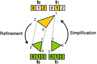
In order to minimise the amount of information that is necessary to represent the different LoDs, the simplified leaves share the vertices of the original ones. The leaf simplification operation eliminates two leaves and creates one single leaf (Figure 2), the two initial leaves would be defined by the triangles t₀ and t₁. If the application requires a reduction in the detail, only one leaf would be rendered using vertices 0 and 2 from t₀ and vertex 1 from t₁. In this way, the new leaf will be rendered using the same array of vertices. It is important to mention that, in this example and in the following ones, the values 0, 1 and 2 that are used to represent a triangle refer to the first, second and third vertex of that triangle, respectively.

Figure 2. Simplification and refinement operations applied to two leaves represented by the triangles t₀ and t₁.

The inverse operation, refinement, is also performed in PT in order to add detail to the current approximation by traversing the stored vertices. The algorithm allows one to both simplify and refine the rendered LoD. Finally, the model can render n approaches in real time with different resolutions, such as the most detailed representation of the leaves of the plant, P₀, and a finite set of coarser approximations P₁, P₂, …, P_{n − 1}. Then the final PT representation P^r stores n approaches.

Initially, the original foliage, P, will be formed by the vertices, V, and leaves, L, of the representation with maximum detail. Let V and L be the sets of vertices and leaves that form the original object, respectively, and let V₀ be the set of vertices of the most detailed representation. Therefore, Equation (1) can be constructed as:

(1)

A PT representation does not store any information about the leaves, because their representation is implicit to the storage order of the vertices in the GPU. Then, the multi-resolution representation P^r will be formed only by the array of vertices. Let V^r be the set of all the vertices used to represent all the different approaches that are stored by P^r. Due to the fact that the multi-resolution model does not add new vertices to the model, Equation (2) can be constructed as:

(2)

Building a PT representation has to be performed in several stages. Initially, the set of leaves defined as quadrilaterals is converted into triangles. Then, the vertices are clustered in a hierarchical structure of bounding boxes in order to find a simplification sequence that fits our representation. Finally, the vertices that define the triangles will be uploaded to the GPU to obtain an interactive visualisation.

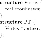
5. Data structure

Geometric data describing the model are stored and processed only in the graphics card. The basic data structure of PT is then simply a vector of vertices in the GPU. The vector stores all the coordinates of the vertices that form the foliage in the original model. The data structure is illustrated in Figure 3. Although it is organised hierarchically, the vertices of the leaves are stored linearly in order to enable the operations of eliminating and recovering vertices of the LoD.

Figure 3. Data structure stored in the memory of the graphics card.

The original representation stores three geometric coordinates, three normal coordinates and two texture coordinates for each vertex, and four indices for each vertex of the leaf. Let ∣V∣ be the number of the vertices in the original representation. The number of leaves in the original approximation can be expressed as ∣V∣/4. Then, taking all these statements into account, the storage cost of the original structure ∣P∣ representation is 9∣V∣.

The use of the PT scheme offers a storage cost that is even lower than the original. This method does not store the indices of the leaves. This approach only needs the data related to the vertices and some additional information for managing the LoD.

Each leaf in a PT representation is represented by only three vertices. Let ∣V^r∣ be the number of vertices stored in the multi-resolution structure, then

(3)

Moreover, in a PT representation, only three geometric coordinates are stored for each leaf. The normal and the texture coordinates are calculated in real time for each vertex. As the data structure shows, a multi-resolution representation P^r is only formed by the original vertices, so:

(4)

Applying Equation (3), the cost of a PT representation is

(5)

Therefore, the storage cost of the original structure ∣P^r∣ representation occupies about 2.25∣V∣. This means that the total cost of storage of P^r is about 75% lower than the cost of the original storage.

6. Pre-processing

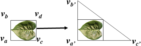
In order to perform the extraction of the correct information, the vertices that form the object are arranged in a pre-process scheme. Their storage order conditioned the different approximations of the foliage. Initially, the original set of leaves, defined as textured quadrilaterals, is converted into triangles. Each new triangle has an area that includes the original quadrilateral, so it contains the texture of a leaf without any distortion. This step is performed in order to reduce the size of the array that stores the vertices, and therefore simplify the storage of the model.

Figure 4 shows an example of converting a leaf initially formed by four vertices into another one made up of three vertices. After this conversion, each leaf of this model is identified by the three vertices that define it.

Figure 4. Conversion of a leaf made up of two triangles into one triangle.

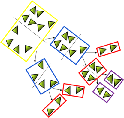
Once the representation has been converted into triangles, the next step is to obtain an ordered sequence of the vertices that form the approximation. This is performed by clustering the leaves by pairs and, following a visibility criterion (see Castelló et al. 2006 for details), writing the ordered vertices of these pairs of leaves in the hardware graphics. This sorting is needed to be able to manage and adapt the LoD of the foliage properly.

Algorithm 1 presents the pseudo-code of this process. The sorting function takes as input a set of leaves, leaves, surrounded by a 3D-oriented bounding boxes (OBBs). It finally creates a hierarchical structure of OBBs that contains all the leaves in the foliage. After the division process, performed by the function Visibility_Division, each bounding box is divided into two news OBBs (OBB1 and OBB2) following the visibility criterion. Each one has to contain an even number of leaves, and to store at least two leaves (min_leaves). Moreover, the number of leaves contained in each OBB resulting from the division process must be equal or differ by two.

Our implementation uses hardware occlusion queries to obtain the number of pixels that pass the z-buffer test. This part of the process is carried out in the GPU. This process makes it possible to perform an ordination of the bounding boxes based on the visibility value, vis(OBB), from the most to the less visible ones.

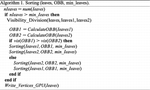
Following the example shown in Figure 5, the set of 10 initial leaves is enclosed in their own OBBs, which is recursively divided until each one contains two leaves and their vertices are stored in the GPU. Then, the vertices of the leaves in the most visible OBBs are stored in the top positions of the vertex array (function Write_Vertices_GPU), followed by the vertices of the leaves of the other boxes, ordered according to their visibility.

Figure 5. Example of calculating hierarchical structure OBBs that represents a sorting process. Each OBB division is shown in different colours.

After this process, three consecutive vertices stored in the GPU form a leaf. This sequence is used to obtain the required approximation of the foliage. The rendering algorithm of PT reduces the LoD by eliminating leaves from the end to the first position. This means that the most visible leaves will be the last ones to be simplified.

7. Run-time processes

Once the vertices have been sorted, the PT has to be able to render a particular LoD on demand. This is performed in real time. The processes that the PT performs in order to extract and render the required approximation are explained in this section.

7.1. Retrieval of the required approximations

As said in Section 4, the multi-resolution model changes the LoD of the foliage by traversing the vertex array with a particular increment. Refining and coarsing operations are performed by managing the list of vertices previously stored in the graphics hardware. These processes provide a conditional hierarchical structure of the leaves that forms the different approximations of the foliage. The leaves are organised as a binary tree structure (Figure 6).

Figure 6. Sequence of original leaves (labelled from t₀ to t₅) and the binary tree obtained after the complete simplification process. The different colours determine the level of simplification in the process: original leaves are green coloured, leaves created by collapsing two original ones are yellow coloured and so on.

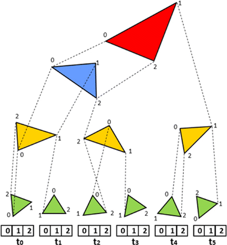
The application calculates the appropriate LoD of the foliage following several criteria, detailed in Section 8. This approximation is formed by a specific number of leaves and, in order to render them, a series of calculations have to be performed. For a better understanding of the LoD retrieval process, this section simulates the LoD retrieval for the leaf organisation shown in Figure 6, while Figure 7 shows the triangles and the vertices that are finally rendered in every LoD.

Figure 7. Trace for the leaf organisation shown in Figure 6

The PT scheme previously stores the vertices that represent the triangles that form the most detailed LoD. These vertices are the only information required in order to render all the possible approximations of the foliage. If some simplification operation has been performed on the foliage, leaves from two successive levels of hierarchy can be rendered. Then, in the rendering stage, the vertex array is traversed twice; the first one for extracting the leaves of the lowest level of hierarchy and the second one for extracting the leaves from the upper level.

Every time the extracting algorithm traverses the vertex array, some parameters have to be established, namely:

• the number of leaves to be rendered in the LoD, nleaves;

• the number of vertices that have to be traversed in this retrieval, nv;

• the step we use to traverse the vertices, step; and

• the starting position, init.

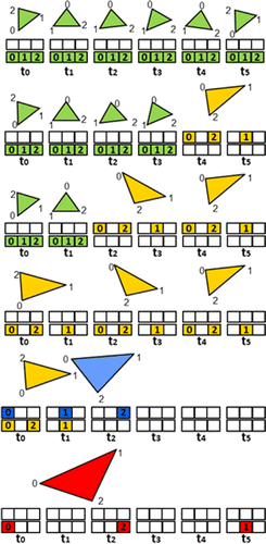
Regarding this example, the values of these parameters are shown in Table 1. It shows the data calculated in order to retrieve the required LoD, formed by a particular number of leaves, nleaves. Although these parameters are not part of the data structure of a PT representation, they are analysed in Table 1 for a better understanding of how different LoD are obtained.

Table 1. Trace of the algorithm.

LoD	nleaves	nv1	nv2	step1	step2	init1	init2
Pn	6	18	0	1	0	0	0
Pn+1	5	12	3	1	2	0	12
Pn+2	4	6	6	1	2	0	6
Pn+3	3	9	0	2	0	0	0
Pn+4	2	3	3	2	4	0	0
Pn+5	1	3	0	8	0	0	0

In the example, the most detailed LoD, P_n, is formed by six leaves. They are green coloured in Figure 6. All the leaves are from the same hierarchy level, the lowest in the binary tree. The number of vertices to be rendered is 18 and, in this case, the vertex array is traversed only once from position 0 following a step of 1. As only one traversing of the vertex array is required, the parameters for the second pass are set to 0.

Every time the LoD is reduced, the two less visible leaves disappear and a new leaf appears. The next LoD, P_{n +1} is formed by one leaf less: the two rightmost leaves, t₄ and t₅, disappear and a new leaf appears in this LoD. In this case, leaves from two different levels of hierarchy are rendered. In Figure 7, the leaves in this upper level of the hierarchy are represented in yellow. In order to render the last leaf of this LoD, the algorithm has to traverse this vertex array again starting from position 12 and extracting three vertices that will form one leaf, and using a step of 2. This step, step2, is obtained from step1 multiplied by 2.

At the next change of level, P_{n +2}, only four leaves have to be rendered. Again, the leaves that disappear are the two rightmost ones from the lowest level of hierarchy in the binary tree, that is to say, t₂ and t₃. The vertex extracting process is similar to the one explained earlier. In the first traversing, the extraction algorithm sends six vertices to be rendered, starting from the first position and using a step of 1. The rest of the leaves is on the upper level of hierarchy in the binary tree. In order to render them, the vertex array is traversed from position 6, extracting six more vertices but following a step of 2.

The LoD P_n+3 is made up of three leaves. The leaves that disappear are the rightmost on the lowest level, that is, t₀ and t₁. In this case, no leaf is rendered from this level of the hierarchy. Then all the leaves are situated on the second level of the hierarchy. From this level, nine vertices are rendered, starting from position 0 and following a step of 2. This is the only traversing that is performed in the vertex array.

A special case appears when an odd number of leaves from the same hierarchy are being rendered and a leaf simplification has to be performed. This case happens when P_n+4 has to be rendered. Here, the new leaf discards the vertices of the rightmost leaf in the current LoD and takes the vertices from the two preceding leaves. Therefore, in the rendering stage, three vertices are traversed from position 0 in the vertex array using a step1 of 2. In order to render the last leaf of the LoD, the algorithm has to traverse this vertex array again starting from position 0 and extracting three vertices that will form one leaf, and using a step of 4.

Finally, P_{n +5} consists of only a single leaf. This is obtained by simplifying the two leaves that appear in the previous LoD P_n+4. In this case, only three vertices are rendered, which is obtained by traversing the vertex array from position 0 with a step of 8.

7.2. Calculating the basic information for leaf retrieval

Once the retrieval example has been analysed, it can be deducted that every variable in Table 1 can be obtained performing some mathematical operations. These are explained next.

• nv1: number of vertices to be traversed on the lowest level of the binary tree;

• nv2: number of vertices to be traversed on the highest level of the binary tree with knowledge of the number of vertices to be drawn in the first stretch #v1, those which form the second #v2 are obtained by using the following formula:

(6)

• step1: increment used to traverse the first stretch of the vector;

• step2: increment with which the second stretch of the vector is traversed. The value of step2 is obtained by multiplying the step of the first stretch by two:

(7)

• init1: the starting position for the first traversing of the vertex array. Its value is always 0;

• init2: in the case of an approach that shows leaves from two different levels of the hierarchy, this parameter contains the starting position from which the second traversing starts. This value will be different depending on whether the number of vertices belonging to the first stretch to be traversed is odd or even. Before performing the simplification operation, the number of leaves of the first level is checked. If this number is odd, the rightmost leaf of the first level is not taken into account, so the two leaves involved in the simplification process are the two preceding ones (Equation 8). Equation (9) reflects the operations performed if this number is even. In this case, the two leaves which are simplified are the two rightmost ones in this first level.

Let i_leaves be the total number of leaves in the original representation.

1. If the number of vertices belonging to the first stretch is odd, the applied formula will be

(8)

1. If the number of vertices belonging to the first stretch is even, the formula applied will be

(9)

As shown above, the data required to obtain a particular approximation are based on two main parameters, which have been denominated nv1 and step1. If these data are known, the rest of the parameters can be calculated easily.

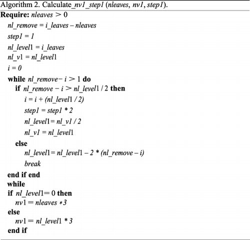
Algorithm 2 shows that how the required data are obtained based on the final leaves to be rendered in the required LoD, nleaves. The algorithm calculates the level of the hierarchy that the leaves of the first traversing performed to render the required leaves belong to. Then, depending on this level, the values step1 and nv1 are obtained.

8. Rendering algorithm

The multi-resolution model proposed here was designed to render uniform levels of detail of foliage. The design can be easily applied to render variable resolutions, that is, different LoDs being rendered in different parts of the foliage.

When a uniform change in the geometry has to be performed, the number of rendered leaves is reduced or increased in some part of the foliage according to the simplification sequence obtained in the pre-processing. The LoD of the foliage is conditioned by a set of criteria. In the PT scheme, the size of the projection of the OBBs that surrounds the whole foliage is taken into account to determine the LoD of this part of the tree. If the projection exceeds a certain size, established by the user, the foliage is rendered with the most detailed representation. The detail of the foliage is reduced following a linear function linked with this projection.

The function Evaluate_prj_OBB(Foliage) returns a floating-point value in the range [0.0, 1.0]. This value is related to the LoD of the foliage. The most detailed representation is rendered when this function returns 1.0, and the coarser representation is visualised when the returned value is 0.0.

(10)

Any time the view conditions change in the scene, the application calculates the appropriate LoD of the object using Function 10. If the LoD that is required differs from the current LoD, the rendering algorithm has to update the detail of the object. The function Calculate_Leaves takes a floating-point number in the range [0.0, 1.0] as input and calculates the number of leaves of the LoD to be rendered.

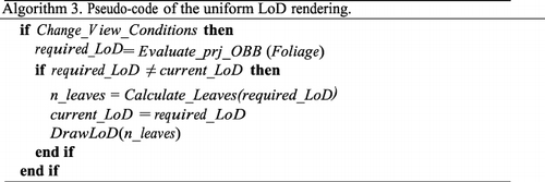
Algorithm 3 presents the pseudo-code of the rendering algorithm for obtaining the appropriate uniform LoD.

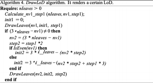
Function DrawLoD is responsible for visualising the leaves that represent the required LoD. This function is shown in the Algorithm 4. It performs the necessary calculations to finally render the leaves by means of the function DrawLeaves. This function takes three parameters to render the foliage: (1) the starting vertex when traversing the vertex array, (2) the number of vertices to be traversed and (3) the increment used in order to render the necessary vertices. In some cases, the leaves from two different levels of hierarchy in the binary tree are drawn, so for these cases the necessary calculations are performed twice with the appropriate parameters.

9. Instantiation

In a real forest, one vegetal species is usually predominant over the others that appear in the ecosystem (see Deussen et al. 2002). This fact is easily represented using the PT scheme. One of the most important contributions of this multi-resolution representation is the simplicity with which different instances of the same vegetal species can be represented without an excessive increment in the storage cost.

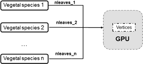
In this representation, the geometry that forms the foliage is stored once per vegetal species. In order to represent different instances of the same species, only the data used to retrieve the vertices of the current approximations are calculated for every one of the different representations, and these data are used to retrieve the appropriate LoD of each instance. Thus, by traversing the same vector ‘vertices’ with different retrieval information, different representations of the same vegetal species will be obtained. Figure 8 represents the data structure of PT involved in the rendering of a natural scene represented by three instances of the same species.

Figure 8. Representation of three instances of the same vegetal species with PT. Each instance is represented with a previously determined number of leaves (nleaves_1, nleaves_2, …).

The process of rendering a prairie using PT representation is very fast because the extraction time is virtually negligible. The bottleneck that exists in most representations due to the traffic of information from the CPU to the graphics system has been virtually eliminated by direct calculations on GPU. Moreover, the spatial cost of representing a forest formed by different representations of a single vegetal species is practically the same as if only one plant is rendered. The increment in the spatial cost is very small, because the geometry of the original model is stored only once in the GPU.

10. Progressive transmission

In virtual globes, it is usual to perform an initial render from a camera situated very far away, as in Google Earth™. In this case, the vegetation that can be seen is rendered with the coarser LoD. As the virtual globe camera becomes closer to the earth, these vegetal species change their resolution and more detail is needed in order to keep the realism. In order to adapt the LoD of each vegetal species to the required by the view conditions, some data that form the vegetal species have to be transmitted over the network, performing a progressive transmission of the geometry. The PT scheme presented here makes this possible, following a client–server architecture. The client computer determines the appropriate LoD for every one of the plants in the virtual landscape according to the rendering conditions, as can be the camera position (cam_position) and the plant position (plant_position). Algorithm 5 details the processes performed in the client computer.

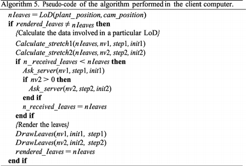
Every time the rendering conditions are changed, the number of leaves of every plant has to be established, according to its importance in the scene. If the rendered LoD has to be updated, the data required to render the new LoD are specified. Functions Calculate_stretch1 and Calculate_stretch2 calculate all the data involved in the rendering of that approximation. If the data stored in the client computer memory are not enough to render the required LoD, the client asks for this information to the server (Ask_server).

The processes performed in the server computer are detailed in the Algorithm 6.

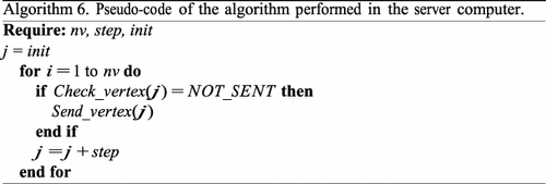
Each one of the required vertices is checked in order to determine if it has been previously sent to the client. If not, this vertex is sent and allocated in the vertex array of the client computer. If two stretches of the vertex array are required, this function is performed twice: one for checking the vertices that form the first stretch and another one for the vertices that form the second one. When the client has all the needed information, the required LoD is rendered, and the number of rendered leaves is updated.

This progressive transmission makes the PT scheme appropriate for rendering vegetation in virtual applications, such as Google Earth™.

11. Results

In order to prove the validity of the proposed model, we aim to verify not only the low storage cost and the fast extraction and visualisation processes, but also the visual quality of the resulting approximations. All the experiments were carried out using Windows 7 on a PC with a processor at 2.8 GHz, 6 GB RAM and an nVidia GeForce 480 GTX graphics card. The environment represented in our tests is the scenario surrounding the Palau of the Arts, in the city of the Arts and Science, Valencia, Spain (Figure 1). A virtual walk-through can be seen at http://cevi.dlsi.uji.es/walkthrough.avi.

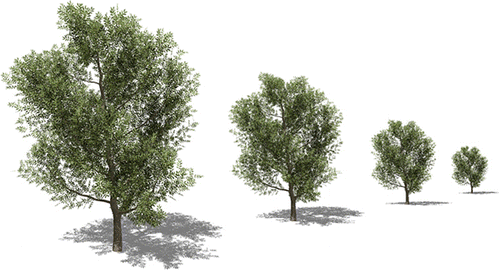
Figure 9 shows different levels of detail (from left to right 100%, 75%, 50% and 25% of the highest detail) of some of the different vegetal species used in our tests. The LoD of each tree is adjusted to the appropriate rendering distance in order to show the effective visual appearance of our rendering method. These results prove that our simplification algorithm is able to maintain the shape and the appearance of the original vegetal species even at 25%.

Figure 9. A composition of different vegetal species at different resolutions placed in the scene at different distances. From left to right, the approximations are represented by the 100%, 75%, 50% and 25% of leaves from the original representation.

Table 2 shows a comparative analysis of the storage cost of vegetal species with different amount of leaves. Here, the storage cost of our algorithm is less than the original unprocessed model. First, our plant representation scheme only uses three vertices per leaf instead of four. Moreover, the texture coordinates for each vertex are calculated in the vertex processing stage on the fly, using 1 byte per vertex for discriminating the vertices. Then our algorithm also saves the storage cost introduced by storing two floating-point values per vertex for texturing. The last column in Table 2 shows the transmission cost of each tree, using a progressive transmission approach, taking into account that 10 bits per vertex component are used to encode each leaf, which is proved to be precise enough for sparse geometry such as the foliage (see Akenine-Möoller et al. 2008 for details).

Table 2. Storage cost comparison (MB) between the original model (Xfrog), our method and the method using progressive transmission. The total number of leaves (Leaves) is also detailed in the table.

Vegetal species	Leaves	Xfrog (MB)	Our method (MB)	Progressive transmission (MB)
Spanish broom	10,740	1.55	0.73	0.30
Manna ash	28,645	4.15	1.96	0.81
Pistacia lentiscus	5594	0.81	0.38	0.16
Olive tree	16,107	2.33	1.10	0.46

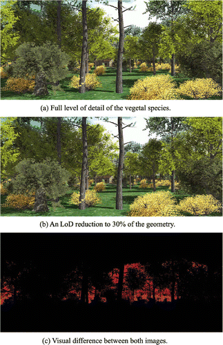
With the aim of showing the visual quality of our algorithm in a real application, we have constructed a forest composed of 1250 instances of different tree and shrub species (shown in Table 2). The amount of triangles used to represent the foliage of the whole scene is 37.5 million triangles. Figure 10 provides a visual analysis of this scene comparing the difference between full detailed representations and PT. Figure 10c shows the per pixel differences between both, showing that the LoD is adapted to the distance. It can be seen that our algorithm is able to reduce the overall geometry of the forest to a 30% of the original geometry without affecting the perceived appearance of the forest. Thus, it can be observed how the instances located in the background have a higher error and how this error is almost visually imperceptible.

Figure 10. A scene of a virtual landscape; Up: full level of detail of the vegetal species; middle: an LoD reduction to 30% of the geometry; down: visual difference between both images.

Finally, a performance comparison of our method with a no-LoD approach can be found in Figure 11. The scene used in this test is the forest shown in Figure 10 with a variable amount of tree instances. The performance of the test is measured taking into account the increasing number of trees in the scene. It can be seen that our method outperforms the approach without LoD in all cases, keeping the frame rate over the 24 fps mark, unlike the technique without LoD whose performance falls below the real-time frame rates.

Figure 11. Performance analysis of our method compared to an approach without LoD.

12. Conclusions and future work

A new continuous multi-resolution model for the representation of the foliage, called PT, has been presented in this paper. This LoD representation can be easily integrated in any virtual globe software, and it can represent interactive virtual species in a realistic way. This is due to the fact that PT considerably reduces the storage cost of the plant by allowing the application to change the detail of the object in a continuous way. The change from one resolution to another is made possible simply by performing some mathematical calculations, detailed in Section 7.2. The storage cost is then considerably reduced in comparison to the LoD schemes based on geometry that have appeared in the literature (Rebollo et al. 2007; Gumbau et al. 2011; Remolar et al. 2012). This is due to the fact that the data required to render a particular LoD is obtained in real time. Another advantage of the PT scheme is that it makes it possible to extract and render the required LoD in a negligible amount of time.

Moreover, PT allows the application to render ecosystems with hundreds of instances of the same vegetal species without increasing the storage cost. The multiple instances are rendered with the appropriate LoD by accessing the data about the object that have been previously stored in the GPU.

A progressive transmission of the geometry can also be performed by means of this multi-resolution model. This fact makes it appropriate to render vegetation in virtual globes. PT allows to visualise a coarse approximation of the plant, transmitting the vertices that form the most detailed approximation only, when these refined LoD are required. The detail of the vegetal species increases as the camera moves towards it. Finally, when the observer is close to the plant, this is rendered with its most detailed LoD.

As future research, we are working on the illumination and shadowing of outdoor scenes for virtual globes. We are working on improving the visual quality of real-time 3D representation of trees by adding to the presented LoD scheme other real-time techniques such as ambient occlusion, soft shadows on the leaves or transparencies.

Acknowledgements

This work was supported by the Spanish Ministry of Science and Technology (Project TIN2010-21089-C03-03) and Feder Funds and Generalitat Valenciana (Project PROMETEO/2010/028).

References

- Akenine-Möoller, T., E. Haines, and N. Hoffman. 2008. Real-Time Rendering. 3rd ed. Natick, MA: A.K. Peters, Ltd.
- Bailey, J. E., and A. Chen. 2011. “The Role of Virtual Globes in Geoscience.” Computers & Geosciences 37 (1): 1–2. doi:10.1016/j.cageo.2010.06.001
- Behrendt, S., C. Colditz, O. Franzke, J. Kopf, and O. Deussen. 2005. “Realistic Real-Time Rendering of Landscapes Using Billboard Clouds.” Computer Graphics Forum 24 (3): 507–516. doi:10.1111/j.1467-8659.2005.00876.x
- Castelló, P., M. Sbert, M. Chover, and M. Feixas. 2006. “Techniques for Computing Viewpoint Entropy of a 3D Scene.” In Lecture Notes in Computer Science 3992, edited by V. N. Alexandrov, G. D. Albada, P. A. Sloot, and J. Dongarra, 263–270. Berlin: Springer-Verlag.
- Cozzi, P., and K. Ring. 2011. 3D Engine Design for Virtual Globes. 1st ed. Boca Raton, FL: CRC Press.
- Dachsbacher, C., C. Vogelgsang, and M. Stamminger. 2003. “Sequential Point Trees.” ACM Transactions on Graphics 22 (3) 657–66210.1145/882262.882321.
- Decaudin, P., and F. Neyret. 2004. “Rendering Forest Scenes in Real-Time.” Rendering Techniques '04 (Eurographics symposium on Rendering), Eurographics Association, Norrköping, Aire-la-Ville, June 21, pp. 93–102.
- Decaudin, P., and F. Neyret, 2009. “Volumetric Billboards.” Computer Graphics Forum 28 (8): 2079–2089. http://hal.inria.fr/inria-00402067.
- Deng, Q., X. Zhang, G. Yang, and M. Jaeger. 2010. “Multiresolution Foliage for Forest Rendering.” Computer Animation and Virtual Worlds 21 (1): 1–23. doi:10.1002/cav.283
- Deussen, O., C. Colditz, M. Stamminger, and G. Drettakis, 2002. “Interactive Visualization of Complex Plant Ecosystems.” VIS'02: Proceedings of the conference on Visualization 2002, 219–226. IEEE Computer Society, Boston, MA, October 27.
- García, I., G. Patow, L. Szirmay-Kalos, and M. Sbert, 2007. “Multi-layered Indirect Texturing for Tree Rendering.” In Eurographics Workshop on Natural Phenomena, edited by D. Ebert and S. Mérillou, 55–62. Aire-la-Ville: Eurographics Association.
- Google Earth 6, 2012. http://www.google.com/earth/explore/showcase/trees.html.
- Gumbau, J., M. Chover, I. Remolar, and C. Rebollo. 2011. “View-Dependent Pruning for Real-Time Rendering of Trees.” Computers & Graphics 35 (2): 364–374. doi:10.1016/j.cag.2010.11.014
- Hoppe, H. 1996. “Progressive Meshes.” SIGGRAPH'96: Proceedings of the 23th annual conference on Computer Graphics and Interactive Techniques, New Orleans, LA, 99–108. Aire-la-Ville: ACM Press, August 4.
- Lacewell, J. D., D. Edwards, P. Shirley, and W. B. Thompson. 2006. “Stochastic Billboard Clouds for Interactive Foliage Rendering.” Journal of Graphics, GPU, and Game Tools 11 (1): 1–12. doi:10.1080/2151237X.2006.10129213
- Linz, C., A. Reche-Martinez, G. Drettakis, and M. Magnor. 2006. “Effective Multi-Resolution Rendering and Texture Compression for Captured Volumetric Trees.” In, Proceedings of the Eurographics Workshop on Natural Phenomena, edited by E. Galin and N. Chiba, 16–21. Aire-la-Ville: Eurographics Association.
- Mantler, S., and A. L. Fuhrmann. 2003. “Fast Approximate Visible Set Determination For Point Sample Clouds.” Proceedings of the workshop on Virtual environments 2003, EGVE'03, Zurich, 163–167. New York: ACM, May 22.
- Meyer, A., F. Neyret, and P. Poulin, 2001. “Interactive Rendering of Trees with Shading and Shadows.” Eurographics workshop on Rendering, London, 183–196. Aire-la-Ville: Springer-Verlag, June 25.
- Neubert, B., S. Pirk, O. Deussen, and C. Dachsbacher. 2011. “Improved Model and View-Dependent Pruning of Large Botanical Scenes.” Computer Graphics Forum 30 (6): 1708–1718. doi:10.1111/j.1467-8659.2011.01897.x
- Paraskevas, T. 2011. “Virtual Globes and Geological Modeling.” International Journal of Geosciences 2 (4): 648–656. doi:10.4236/ijg.2011.24066
- Rebollo, C., I. Remolar, M. Chover, J. Gumbau, and O. Ripollés. 2007. “A Clustering Framework for Real-Time Rendering of Tree Foliage.” Journal of Computers 2 (4): 57–67. doi:10.4304/jcp.2.4.57-67
- Reche, A., I. Martin, and G. Drettakis. 2004. “Volumetric Reconstruction and Interactive Rendering of Trees from Photographs.” ACM Transactions on Graphics (SIGGRAPH Conference Proceedings) 23 (3): 720–727. doi:10.1145/1015706.1015785
- Remolar, I., J. Gumbau, M. Chover, and C. Rebollo. 2012. “Efficient Management of Forests for Real Time Rendering.” IVAPP 2012: Proceedings of the international conference on Computer Graphics Theory and Applications and international conference on Information Visualization Theory and Applications, Rome, 87–96. Berlin: SciTePress, February 24–26.
- Ribelles, J., A. López, O. Belmonte, I. Remolar, and M. Chover. 2002. “Multiresolution Modeling of Arbitrary Polygonal Surfaces: A Characterization.” Computers & Graphics 26 (3): 449–462.
- SpeedTree, 2012. “Speedtree, Interactive Data Visualization Inc.” http://www.idvinc.com/speedtree/.
- Stamminger, M., and G. Drettakis. 2001. “Interactive Sampling and Rendering for Complex and Procedural Geometry.” In Proceedings of the 12th Eurographics Workshop on Rendering Techniques, edited by S. Gortler and C. Myszkowski, 151–162. London: Springer-Verlag.
- To, D. S. P., R. W. H. Lau, and M. Green. 1999. “A Method for Progressive and Selective Transmission of Multi-Resolution Models.” VRST'99: Proceedings of the ACM symposium on Virtual Reality Software and Technology, London, 88–95. New York: ACM Press, December 20–22.
- Wand, M., M. Fischer, I. Peter, F. Meyer auf der Heide, and W. StraBer. 2001. “The Randomized z-buffer Algorithm: Interactive Rendering of Highly Complex Scenes.” SIGGRAPH’ 01: Proceedings of the 28th annual conference on Computer Graphics and Interactive Techniques, Los Angeles, 361–370. New York: ACM Press, August 12–17.
- Xfrog, 2012. “Greenworks: Organic Software.” http://www.greenworks.de/.