Evaluation of global land cover maps for cropland area estimation in the conterminous United States

Abstract

Global land cover data could provide continuously updated cropland acreage and distribution information, which is essential to a wide range of applications over large geographical regions. Cropland area estimates were evaluated in the conterminous USA from four recent global land cover products: MODIS land cover (MODISLC) at 500-m resolution in 2010, GlobCover at 300-m resolution in 2009, FROM-GLC and FROM-GLC-agg at 30-m resolution based on Landsat imagery circa 2010 against the US Department of Agriculture survey data. Ratio estimators derived from the 30-m resolution Cropland Data Layer were applied to MODIS and GlobCover land cover products, which greatly improved the estimation accuracy of MODISLC by enhancing the correlation and decreasing mean deviation (MDev) and RMSE, but were less effective on GlobCover product. We found that, in the USA, the CDL adjusted MODISLC was more suitable for applications that concern about the aggregated county cropland acreage, while FROM-GLC-agg gave the least deviation from the survey at the state level. Correlation between land cover map estimates and survey estimates is significant, but stronger at the state level than at the county level. In regions where most mismatches happen at the county level, MODIS tends to underestimate, whereas MERIS and Landsat images incline to overestimate. Those uncertainties should be taken into consideration in relevant applications. Excluding interannual and seasonal effects, R² of the FROM-GLC regression model increased from 0.1 to 0.4, and the slope is much closer to one. Our analysis shows that images acquired in growing season are most suitable for Landsat-based cropland mapping in the conterminous USA.

Keywords:

• cropland area
• global land cover
• FROM-GLC
• area estimation
• NASS survey

1. Introduction

Covering about 12% of the Earth's land surface (FAO 2012), cropland experienced tremendous expansion in area and uneven geographical reallocation in the past decade (Foley et al. 2011). Changes in cultivated areas, both expansion and degradation, are related closely to social and ecological welfare of human society. Accurate and timely information on the coverage of agricultural lands over various areas of the world is important to a variety of end-users, such as farmers, crop yield predictors, food market researchers, and policy/decision-makers. As the world's population has already exceeded seven billion and continues to grow, monitoring of cropland changes becomes essential for ensuring global food security (Yu 2011; Thenkabail et al. 2012; Yu et al. 2013). In the meantime, issues such as water availability, nutrient runoff, carbon sequestration, and habitat fragmentation have also been cited as resulting from the extend and distribution changes of this land use activity. This causes severe ecosystem dis-service to nature and human health and making profound impacts on biogeochemial cycles and biodiversity (Matson et al. 1997; Tilman et al. 2001; Tscharntke et al. 2005; DeFries et al. 2007; Foley et al. 2011; Gong, Yin, and Yu 2011). The solutions to those problems will require measurements of cropland coverage over various spatial extents such as watersheds and eco-regions, or over political divisions, such as counties and states. Thus, spatially explicit, consistent, and accurate monitoring of the extent and changes of agricultural land is needed.

The value of remote sensing in the development of a viable crop estimator has long been recognized. For instance, since its launch in 1972, images from Landsat 1 were employed in agricultural inventory (Allen 1990; Battese, Harter, and Fuller 1988). Agricultural lands are changing continuously and intensively under the context of global warming and anthropogenic transformation. Cropland mapping at local and regional scales cannot meet the demands of global change studies (e.g. Zhong et al. 2011, 2012, 2014; Boryan et al. 2011), and until now, no effort has been devoted to the time-series fine-resolution global cropland mapping. Under these circumstances, continuously updated global land cover maps, which contain cropland layers at coarse and medium resolution, are alternatives to the monitoring of agricultural land coverage and changes.

Currently, there are four maps that contain dynamic global land cover information: the annual 500-m resolution MODIS land cover maps from 2001 to 2011 (Friedl et al. 2002, 2010); the 300-m resolution GlobCover land cover maps in 2006 and 2009 (Arino et al. 2008); the 30-m resolution Finer Resolution Observation and Monitoring of Global Land Cover (FROM-GLC) with an improved version (FROM-GLC-agg) in 2010 and the 2000 product to be released soon (Gong et al. 2013). Although independent validation efforts have been undertaken within each institution by using their own validation data-sets, performances could be different when evaluated with third-party data (Gong 2008). Additionally, the accuracy of area estimations is not fully compatible with site-specific accuracy results, especially when the accuracy is poor (Hollister et al. 2004).

Annual agricultural survey statistics released by the US Department of Agriculture's (USDA) National Agricultural Statistics Services (NASS) can be treated as good baseline data for area estimation assessment in the USA. Here, we compare those four global land cover products with this survey data to evaluate their performances in cropland area estimation. Because it is impossible to collect less-or-free-of-cloud Landsat images for the entire globe over a season or an individual year, we also assessed the interannual and seasonal effects on accuracy of area estimation from Landsat-based cropland maps. The two main objectives of this research are: (1) providing data selection guidance to users who require crop area estimates at the county or state levels, by characterizing the major strengths and weaknesses of different global land cover products in delivering such estimates; and (2) providing advice to future cropland mapping activities on selection of proper image dates and spatial resolution.

2. Data

2.1. NASS annual agricultural survey

NASS crop surveys are conducted annually by sending questionnaires to farming operations that are selected based upon farm size (>$1000 of agricultural products either produced or sold) and the ownership of commodities of interest. A sample of approximately 65,000–81,000 farm operators is selected, which accounts for approximately 3% of the total population in the USDA census report (USDA National Agricultural Statistics Service 2009). For each state, an adjustment factor is applied to compensate for potential errors introduced by non-responses or incomplete questionnaires, which is allocated subsequently to the county level with a weighting factor (Maxwell, Wood, and Janus 2008). To match the survey data with the cropland classes in the global land cover data-set, we first selected the herbaceous field crops that are equivalent to the cropland definitions in remote sensing products (Table 1). Then we acquired their survey statistics in year 2010 via the NASS web query interface (http://quickstats.nass.usda.gov/, as of 5 February 2013). For each county, we summed the planted acres of those listed items. The planted acres were used because this is more relevant to the land cover type that can be derived from remotely sensed data. Records containing no county name were excluded from the county-level-based analysis, but were agglomerated at the state level.

Table 1. Salient properties of analyzed land cover products and corresponding field crop commodities in the NASS survey data.

Data	Agricultural classes	Class definitions
NASS survey	Field crop commodities	Barley; Beans; Canola; Corn; Cotton; Flaxseed; Hay & haylage; Haylage; Hops; Lentils; Millet; Mint; Mustard; Oats; Peanuts; Peas; Rapeseed; Rice; Rye; Safflower; Sorghum; Soybeans; Sugarbeets; Sugarcane; Sunflower; Sweet corn, processing; Sweet potatoes; Taro; Tobacco; Wheat.
CDL		Alfalfa; Barley; Buckwheat; Camelina; Canola; Corn; Cotton; Double Crop Winter Wheat/Soybeans; Dry Beans; Durum Wheat; Fallow/Idle Cropland; Flaxseed; Hops; Lentils; Millet; Mint; Mustard; Oats; Other Crops; Other Hay/Non Alfalfa; Other Small Grains; Peanuts; Peas; Pop or Orn Corn; Potatoes; Rape Seed; Rice; Rye; Safflower; Sorghum; Soybeans; Speltz; Spring Wheat; Sugar beets; Sugarcane; Sunflower; Sweet Corn; Sweet Potatoes; Tobacco; Winter Wheat.
GlobCover	Post-flooding or irrigated croplands (or aquatic)	Irrigated tree crops; Irrigated shrub crops; Irrigated herbaceous crops; Post- flooding cultivation of herbaceous crops.
	Rainfed croplands	Rainfed shrub crops; Rainfed tree crops; Rainfed herbaceous crops.
	Mosaic cropland (50–70%)/vegetation (20–50%)	Cultivated and managed terrestrial areas/natural and semi-natural primarily terrestrial vegetation.
	Mosaic vegetation (50–70%)/cropland (20–50%)	Natural and semi-natural primarily terrestrial vegetation/cultivated and managed terrestrial areas.
MODIS	Croplands	Lands covered with temporary crops followed by harvest and a bare soil period (e.g. single and multiple cropping systems). Note that perennial woody crops will be classified as the appropriate forest or shrub land cover type.
	Cropland/natural vegetation mosaics	Lands with a mosaic of croplands, forests, shrubland, and grasslands in which no one component comprises more than 60% of the landscape.
FROM-GLC & FROM-GLC-agg	Rice fields	Land for rice cultivation.
	Other croplands	This category includes arable and tillage land.
	Bare herbaceous croplands	Just harvested, fallow land and all other types of land not covered by vegetation such as lake bottoms in dry season.

Note: Class name and definition of croplands in different products are directly copied from original references. Corresponding cropland commodities in NASS survey are under the group of field crops.

2.2. FROM‐GLC

FROM-GLC is a 30-m resolution global land cover map produced from 8903 scenes of Landsat TM/ETM+, of which, approximately three quarters is circa 2010 and one-quarter is circa 2000 (Gong et al. 2013). For the USA, approximately 57% of the images were acquired in 2010. The best overall accuracy (64.9%) checked against independent test samples collected following a systematic unaligned scheme was achieved with a support vector machine algorithm. The user's accuracy (UA) and producer's accuracy (PA) for cropland are 45% and 39%, respectively. This set of the FROM-GLC product shares three categories of croplands that can be matched to the NASS survey items: rice fields, other croplands, and bare herbaceous croplands.

2.3. FROM‐GLC‐agg

An improved version of FROM-GLC was released at the same time by integrating a map derived with a segmentation-based approach, a nighttime light impervious surface area map and a MODIS urban extent map (Yu et al. 2013). This aggregation map, called FROM-GLC-agg, was validated by the same set of test samples. The overall accuracy was raised to just 65.51%, but the UA and PA for cropland have been substantially improved to 58% and 67%, respectively. This improvement was due largely to the inclusion of both phenological information in the MODIS EVI time-series and bioclimatic variables in the classification (http://data.ess.tsinghua.edu.cn/, as of 29 October 2013). The classification system in FROM-GLC-agg was adopted from FROM-GLC, and thus the same set of classes is selected.

2.4. MODIS land cover product

The Collection 5.1 MODIS Global Land Cover Type product (MODISLC) has been generated on a calendar year basis from 2001 to 2011 at 500-m resolution using a supervised classification tree algorithm (Friedl et al. 2010). This product was refined by certain post-processing steps. For instance, year-to-year variation in land cover labels not associated with real land cover changes was constrained by a stabilization technique using posterior probabilities (Friedl et al. 2010). A 10-fold cross-validation resulted in 75% overall accuracy. We chose the land cover layer in year 2010 with the International Geosphere-Biosphere Programme classification scheme because its ancillary information, such as confusion matrix, had been provided by Friedl et al. (2010). This scheme distinguishes 17 categories of land cover of which cropland and cropland/natural mosaic are agricultural. The user's accuracies for the two classes are 83% and 60% and the producer's accuracies are 93% and 27%, respectively (recalculated from Table 4 in Friedl et al. 2010).

2.5. GlobCover 2009 product

GlobCover2009 is the second edition of the European Space Agency's global land cover maps produced with 300-m resolution MERIS fine resolution surface reflectance mosaic covering the entire year of 2009. The globe is split into 22 strata and a two-step classification was run for each stratum independently, which consists of a supervised step identifying poorly represented classes and an unsupervised clustering on the remaining pixels. The data coverage in the USA is uneven because of programmatic constraints, which give a relatively higher image acquisition rate in the northwest region and a lower rate in the southeast (Bontemps et al. 2011). The GlobCover 2009 legend follows the United Nations Land Cover Classification System (LCCS) with 22 classes, of which four are related to the NASS categories: post-flooding/irrigated croplands, rain-fed croplands, mosaic cropland (50–70%)/vegetation, and mosaic vegetation (50–70%)/cropland. In the validation report of GlobCover, we noticed that two LCCS types, ‘Irrigated tree crops’ and ‘Irrigated shrub crops’ are included in ‘Post-flooding or irrigated croplands (or aquatic)’, while ‘Rainfed shrub crops’ and ‘Rainfed tree crops’ are under ‘Rainfed croplands’. We realized that tree and shrub crops were not comparable with the selected NASS classes, but there is no feasible way for us to separate them from the remaining herbaceous crops with the current version. Thus, we expect that the assessment on GlobCover in this paper would be overestimated, but the magnitude is hard to estimate because there is no information about the area proportion of tree and shrub crops in each category. For consistency, we used the 2009 NASS survey data for assessment of the GlobCover product.

3. Methods

3.1. Area estimation from global land cover data

Various methods have been proposed for area estimation from remotely sensed data. The most intuitive approach is pixel counting. This method multiplies the number of pixels grouped into certain types by the area of each pixel, which can introduce bias either through the presence of mixed pixels or the misclassification of pure pixels (Czaplewski 1992; Carfagna and Gallego 2005). For coarse resolution maps like MODIS, this effect is even severe (Friedl et al. 2010). Some studies corrected the proportion of croplands in each pixel by looking up for their original legend descriptions (e.g. Hannerz and Lotsch 2008). This approach is feasible at small-scale studies where the landscape is relatively homogeneous, but would become problematic if the proportion of cropland and other land cover mosaic classes is not geographically even. Another way of calibration is to use confusion matrix (Stehman 2013), but this can be difficult because of the limited source of structured ground data applicable to multiple scales. An alternative is to use ratio estimators (Hanuschak et al. 1980), a ratio of the higher accuracy variable over a lower one, to adjust the area estimates (Lathrop 2006). It is suggested that misclassification bias in areal estimates from remotely sensed data can be corrected by employing statistically based calibration techniques and independent reference data (Czaplewski 1992). Here, the MODISLC and GlobCover estimates were treated as the low accuracy estimates because of their relative coarse resolution, while the NASS Cropland Data Layer (CDL) was considered as the approximately unbiased acreage estimates. As the resolution of the CDL is no higher than FROM-GLC, pixel counting was applied without the use of ratio calibration. The CDL is produced annually through a supervised classification at 30-m resolution, based primarily on data from the Indian Remote Sensing RESOURCESAT-1 sensor collected during the current growing season. The reported PA and UA are 85% to 95%, respectively, for major crop categories (Boryan et al. 2011). The cropland types in year 2010 CDL categories are summarized in Table 1.

The CDL-adjusted crop acreage for land cover products was expressed as a sum of the cropland area for the mixed subtypes, which are reweighted by their ratio estimators. Taking MODISLC for demonstration purposes, the function for the adjusted area estimation is:

(1)

where i is the subscript for county; is the CDL-adjusted cropland estimate for the county; Area_1(i) and are the area estimates for cropland and crop-natural vegetation mosaic, respectively, for the county; β₁ and β ₂ are two unknown ratio estimators, which are estimated by the method of least squares to best fit the model to the CDL survey statistics. The MODISLC and GlobCover adjusted area estimates are named as weighted MODISLC and weighted GlobCover.

3.2. Assessment with NASS survey

A linear regression model was fitted separately for the six pairs of data to capture the pattern of how land cover maps match the USDA NASS survey data at both county and state levels. A Student's t-test was applied to test for the level of significance for the coefficient of determination (R²) and slope. A significant and high R ² value implies that the model fits the data well and that a large proportion of the variability in the data can be explained by the linear model. A regression with a slope not significantly different from one indicates a desired relationship between the two area estimates. In addition to R² and slope, we employed three other indices to represent the direction and magnitude of the estimation differences. Mean deviation (MDev) is the difference between the two measurements, which indicates the overall pattern of a products' estimation: either positive or negative (Goslee 2011). Root mean square error (RMSE) is a generalized standard deviation that measures the absolute difference by squaring the deviation. MDev and RMSE are in units of percentage of county/state area. Relative difference (RD) is similar to MDev, but can indicate the effect of estimation for each political unit. We calculated RD on a county basis and divided the results into three levels: underestimation (RD < −20%), fair estimation (−20% < RD < 20%), and overestimation (RD > 20%). The functions for those calculations are:

(2)

(3)

(4)

where i is the subscript for county; n is total number of counties; and are the cropland acreage estimated from the land cover product and survey data, respectively.

3.3. Interannual and seasonality effects

MODISLC and GlobCover are generated based on an image assemblage collected within a target year. This is in contrast to FROM-GLC and FROM-GLC-agg, which were developed from a temporally patchy Landsat data-set due to limited data availability. It is unclear to what degree the interannual effect has on capacity of these products for cropland area estimation. Another factor that could affect image classification accuracy is the season of image acquisition. Generally speaking, without any time-series information input, the ideal time window for a synthesized global land cover map is the peak of the growing season, during which the spectral signals among various landscape elements are more distinctive. Since global mapping with finer resolution data of limited temporal capacity is emerging, it is necessary to assess these effects to provide guidance on data selection in future efforts of cropland monitoring.

Discounting the potential bias initiated from the sample size, we evaluated the interannual and seasonal effects by comparing the R² and slope of the linear regression model built from two restricted data-sets with those of the full data-set. The full data-set includes data for all counties, whereas the restricted one is its subset. The interannual restricted data-set contains only data from counties that fall completely into the FROM-GLC Landsat scenes collected in 2010, and the seasonal restricted data-set contains data from counties that intersect fully with Landsat images obtained during the growing months. In the USA, the growing season varies significantly depending on crop type and region. By rough reckoning from the USDA 2010 crop progress time-table, we treated May to August as the growing season for major crops (e.g. corn, winter wheat, soybean) (USDA, National Agricultural Statistics Service 2011). For the two comparisons, if significant improvement is found in the results of either restricted data-set compared with the full data-set, it implies that the Landsat-based products have space for further improvement by replacing the images acquired in years/seasons outside the mapping year/growing seasons, with those from the mapping year/growing seasons.

4. Results

4.1. Area estimation from global land cover data

The ratio estimators for MODISLC cropland and cropland mosaic are 0.7 and 0.2, respectively, and for GlobCover mosaic cropland (50–70%)/vegetation and mosaic vegetation (50–70%)/cropland are 0.58 and 0.38, respectively.

4.2. Assessment with NASS survey

County-by-county regressions between the six sets of remote sensing cropland area estimates and NASS cropland survey data are all significant but with large discrepancies (Figure 1 and Table 2). R² ranges from 0.1 to 0.67. Weighted MODISLC exhibits the most variance (0.67) and MODIS ranks third (0.46). Only the slope of MODIS is not significantly different from one, but its overall deviation is the greatest (MDev = 0.29 and RMSE = 0.38), whereas the weighted MODISLC displays the smallest overall deviation among all products. There is little difference in R² between the non-weighted (0.25) and the weighted (0.24) estimations for the two GlobCover sets, but the weighted results are closer to the survey statistics, as indicated by MDev and RMSE. FROM-GLC produces the lowest R² (0.1), whereas FROM-GLC-agg achieves high R² (0.51) and a reduced RMSE value (0.23).

Figure 1. Comparison between NASS cropland survey at county level and estimations from six datasets. Dashed line is 1:1 and the solid line is the regression line.

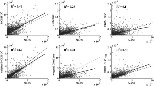
Table 2. Parameters of regression models building from six cropland area estimates and NASS survey at county level. Null hypotheses for the two student's t tests are separately (1) model is not significant and (2) slope is not significantly different from one. We treat p ≤ 0.001 as the significance level. Unite for intercept is 10,000 acre, and for MDev and RMSE is percentage of county area.

	R ^2	p	slope	p	MDev	RMSE
MODISLC	0.459	<0.001	1.021	0.377	0.285	0.381
Weighted MODISLC	0.669	<0.001	0.822	<0.001	0.007	0.113
GlobCover	0.246	<0.001	0.797	<0.001	0.112	0.236
Weighted GlobCover	0.242	<0.001	0.471	<0.001	−0.052	0.201
FROM-GLC	0.100	<0.001	0.584	<0.001	0.108	0.322
FROM-GLC-agg	0.510	<0.001	1.135	<0.001	0.158	0.232

When examined by state, all six data-sets achieve higher R² than those at the county level (Figure 2 and Table 3). FROM-GLC-agg obtains the highest R² (0.95), followed by GlobCover (0.83) and weighted GlobCover (0.81). The correlation coefficient for weighted MODISLC is 0.74. The two lowest values are obtained for MODISLC (0.59) and FROM-GLC (0.54). However, no slope of any of the six data-sets is significantly similar to one, and the absolute deviation of slope from one (y = x line) for all products is larger than that at county level. All data-sets have their MDev and RMSE decreased compared with those at the county level. They all tend to underestimate total cropland area since all MDev are negative.

Figure 2. Comparison between NASS cropland survey at state level and estimation from six datasets. Dashed line is 1:1 and the solid line is the regression line.

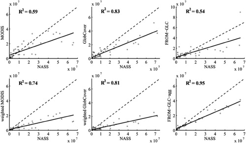
Table 3. Parameters of regression models building from six cropland area estimates and NASS survey at state level. Null hypotheses are the same as Table 2. Unit for intercept is 100,000 acre, and for MDev and RMSE is percentage of state area.

	R ^2	p	slope	p	MDev	RMSE
MODISLC	0.594	<0.001	0.459	<0.001	−0.205	0.317
Weighted MODISLC	0.744	<0.001	0.296	<0.001	−0.031	0.227
GlobCover	0.831	<0.001	0.536	<0.001	−0.105	0.217
Weighted GlobCover	0.806	<0.001	0.288	<0.001	−0.024	0.177
FROM-GLC	0.535	<0.001	0.566	<0.001	−0.089	0.300
FROM-GLC-agg	0.946	<0.001	0.570	<0.001	−0.107	0.205

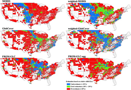
The RD between county-level area estimation and the survey data are diverse spatially (Figure 3). Weighted MODISLC, FROM-GLC-agg, and GlobCover show clusters of good estimation, defined by ±20% RD, in the upper middle-east region. Of the total targeted counties, 33% are well estimated by weighted MODISLC, 20% by FROM-GLC-agg, and 19% by GlobCover. The two lowest values are FROM-GLC (15%) and MODISLC (5%). Under most circumstances, potential users such as food safety managers would expect counties with vast agricultural coverage and higher productivity to be mapped more precisely. Thus, in terms of acreage, the land cover product that produces the highest percentage of well-estimated cropland acreage is weighted MODISLC (25%), followed by weighted GlobCover (16%). The percentage for GlobCover and FROM-GLC-agg are both 14%, and the two poorest performers remain FROM-GLC (11%) and MODIS (5%). Meanwhile, as revealed from Figure 3, in regions where most mismatches between the remote sensing estimation and survey data happen, MODIS tends to underestimate, whereas MERIS and Landsat images incline to overestimate.

Figure 3. Assessment of six datasets with NASS cropland survey at the county scale. The differences between NASS cropland survey and product estimations were represented by relative difference (RD). RD was divided into three levels. Counties with no available survey data are not colored.

4.3. Interannual and seasonality effects

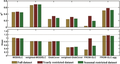
To assess the interannual effect, we compared the slopes and values of correlation coefficient derived from the regression analysis for the full data-set with the yearly and seasonal restricted data-sets (Figure 4). For MODISLC, weighted MODISLC and FROM-GLC-agg, the R² and slope of their two restricted data-sets are not significantly different from those of their full data-sets. In contrast, by using scenes from 2010 only, FROM-GLC shows the most evident improvement in R² and its slope is closer to one.

Figure 4. Bar charts representing R² and slope of the full data-set, yearly restricted data-set and season restricted data-set for each product. The number of counties in the full, yearly restricted, and seasonal restricted datasets are separately 2174, 1419 and 1483.

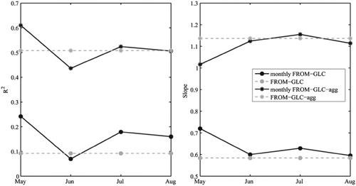
In terms of the evaluation of the seasonal effect, the two Landsat-based products FROM-GLC and FROM-GLC-agg show similar tendency in R² and slope changes (Figure 5). Both achieved the highest R² in May, followed by a significant drop in June, and then stabilized in July and August. The R² of FROM-GLC showed a substantial increase in all growing months except for June, and reached the highest value of 0.24 in May from 0.1 in the full data-set. Judging by the slope, both restricted data-sets have their slope closest to one in May, and slopes from June to August do not show obvious improvement over their full data-set.

Figure 5. Comparison of R² and slope between the full data-set and seasonality restricted data-set of FROM-GLC and FROM-GLC-agg. The gray and dashed lines represent the two full datasets of FROM-GLC and FROM-GLC-agg, while the black and solid lines represent the two restricted datasets. Lines with asterisk marks indicate data derived from FROM-GLC-agg, while lines with circles indicate data derived from FROM-GLC.

5. Discussion

All global land cover products achieve better performance in cropland area estimation at the state level than at the county level, which is manifested by higher correlation coefficients and smaller deviation. There are two possible explanations for this. First, the state-level estimates are considered more accurate than the county-level estimates (Maxwell, Wood, and Janus 2008). The adjustments for potential errors in the NASS survey were generated at the state level, and allocated subsequently to the county level. This design would undoubtedly better adjust the state-level data while introducing more uncertainties at the county level. Second, errors are not scale-invariant in the process of a bottom-up data aggregation unless no error exists, but instead, direct summation would either aggravate or reduce errors by canceling out positive and negative differences. In our case, data aggregation would reduce errors because most points are clustered around the y = x line, as revealed from the scatter plots. In addition, when regressing the country-supplied statistics from the FAO national surveys conducted in 2009 with estimations from FROM-GLC in the top 50 largest countries, the value of R² is up to 0.7 (Gong et al. 2013). However, it decreases to 0.54 at the state level, and to 0.1 at the county level.

We recognize that a better ratio estimator should be adjusted according to the landscape diversity, topographic complexity, and agricultural intensity. However, this paper is not aimed at finding new parameters. Instead, we check for the feasibility of applying ratio estimator to coarse resolution products. Not coincidentally, the ratio estimators for both MODISLC and GlobCover match well with the definitions of the mixed subtypes. For instance, the weights for GlobCover are 0.58 and 0.38, respectively, while the cropland cover in the mosaic cropland/vegetation type is 50–70% and in mosaic vegetation/cropland is 20–50%. This also proves the reliability of this approach. By applying the ratio estimators that are derived based on the 30-m resolution CDL to MODISLC, both MDev and RMSE decrease considerably, and the variance explained by the regression model increases by nearly 20% at both county and state levels. Nonetheless, this improvement is not significant for GlobCover, as revealed from the coefficient of determination, slope, MDev, and RMSE. One possible explanation is that GlobCover was produced based on the MERIS FR surface reflectance mosaics covering six periods in a year. It is quite possible that a county was classified using images from various seasons, and thus a unified ratio estimator applied to the entire country does not work efficiently when compared to MODISLC.

Although 2010 is the nominal mapping year for FROM-GLC and FROM-GLC-agg, Landsat data acquired in 2010 only occupy 33.5% of the total image collection globally, and for the conterminous USA, the proportion increases to 57%. In terms of the percentage of images acquired from May to August, it is 56% at the global level and 63.3% for conterminous USA. Our results indicate, for products without inclusion of any additional phenological information into the classification, both interannual and seasonal effects are significant. In contrast, considering MODISLC, weighted MODISLC, and FROM-GLC-agg, which used time-series information in the classification, their values of R² and slopes did not differ significantly between the restricted and full data-sets. By analyzing only the 2010 data, the R ² of the FROM-GLC increased from 0.1 to 0.4 and the slope improved from 0.35 to 0.98. A similar effect can also be seen when using the seasonal restricted data-set. This implies that with all the other control factors fixed, when determining the classification accuracy, there is plentiful space for improvements in FROM-GLC by using images from the optimal season and/or year. For the conterminous USA, images acquired in May work best because R² was improved significantly and because the slope became closer to one. In general, May is the month marking the onset of crop growth in the mid-latitudes of the Northern Hemisphere. The unique spectral properties of crops in the early growing season make it easier to be distinguished from areas of unmanaged natural vegetation, such as grassland, shrub, and forest, because they are still at the spring budburst stage without abundant biomass. This type of spectral difference will gradually diminish in June when most types of vegetation achieve full growth. After June, grasses become less vigorous, but forests and shrubs continue to thrive. However, confusion between crop and forest/shrub can be avoided better than can confusion between crop and grass by texture or vegetation biomass, and thus, images acquired in July and August are secondary alternates for image selection.

Although large discrepancies exist among these different products, they do show some common trends. They are all inclined to have better performance in topographically flat regions, such as Illinois, Indiana, Iowa, Missouri, South Minnesota, and East Nebraska. Another study in China, which compared estimates of total cropland area from NOAA AVHRR land cover maps with county-level agricultural census data for 1990, reached a similar conclusion (Frolking et al. 1999). They found high correlations between the two sources of data only in the North and Central plains of China, and much weaker correlations in the remaining regions. The mountainous areas of the USA were constituted with more complex and heterogeneous landscapes than flat plains, and the evaluation results of the global land cover products in those regions are distinct from each other, but none is satisfactory. MODIS underestimated a vast coverage of those regions, whereas MERIS and Landsat images showed overestimation. The diversity of terrain in mountainous regions and the fragmented cropland landscape makes it a challenge for land cover mapping using satellite remote sensing.

6. Conclusion

Land cover product can be used in cropland area measurement at various spatial units greater than the original pixel resolution. Crop area estimates at administrative levels (county, province, state, nation) are useful information in many applications such as production management, water resource planning, and disaster response. Using the USDA NASS survey data as a baseline for evaluating the four most recent global land cover products in cropland acreage estimation for the conterminous USA, we found:

1. Remote sensing-derived global land cover products gave better results at the state level than at the county level in cropland area estimation.

2. The choice of input data for downstream analyses depends on geographic regions, spatial extent, and application fields. Weighted MODISLC produces the highest percentage of well-estimated cropland acreage in the USA, followed by weighted GlobCover. For applications that require aggregated data at the county scale, weighted MODISLC will result in the least deviation from the survey, while at the state level, FROM-GLC-agg wins the vote.

3. County-by-county examination shows that the RDs between the cropland area estimated from the global products and the survey data varied spatially in the USA. The discrepancies are high among products. The proportion of counties that matched well with survey data ranges from 5 to 33%.

4. Our ratio estimator approach is feasible with the MODIS land cover product for cropland acreage estimation in the USA, but is not effective with the GlobCover product.

5. Images acquired at the beginning of the growing season are more suitable for cropland mapping with Landsat data in the USA.

6. The conclusions here may or may not be applicable in other parts of the world, since the estimation errors and uncertainties are determined by a large number of factors, such as the complexity of landscape pattern, the agricultural system, the timing, and the weather condition on the day of image acquisition, and the quality of training samples.

Acknowledgment

This research was supported by USGS (grant number G12AC20085). The authors would like to thank four anonymous reviewers for their valuable comments and suggestions to improve the quality of this paper.

References

- Allen, J. D. 1990. “A Look at the Remote Sensing Applications Program of the National Agricultural Statistics Service.” Journal of Official Statistics 6 (4): 393–409.
- Arino, O., P. Bicheron, F. Achard, J. Latham, R. Witt, and J. L. Weber. 2008. “GLOBCOVER the Most Detailed Portrait of Earth.” ESA Bulletin-European Space Agency 136: 24–31.
- Battese, G. E., R. M. Harter, and W. A. Fuller. 1988. “An Error-components Model for Prediction of County Crop Areas Using Survey and Satellite Data.” Journal of the American Statistical Association 83 (401): 28–36. doi:10.1080/01621459.1988.10478561.
- Bontemps, S., P. Defourny, E. Van Bogaert, O. Arino, V. Kalogirou, and J. Ramos Perez. 2011. “GlobCover 2009: Products Description and Validation Report.” European Space Agency. Accessed April 20. http://ionia1.esrin.esa.int/docs/GLOBCOVER2009_Validation_Report_2,2.
- Boryan, C., Z. Yang, R. Mueller, and M. Craig. 2011. “Monitoring US Agriculture: The US Department of Agriculture, National Agricultural Statistics Service, Cropland Data Layer Program.” Geocarto International 26 (5): 341–358. doi:10.1080/10106049.2011.562309.
- Carfagna, E., and F. J. Gallego. 2005. “Using Remote Sensing for Agricultural Statistics.” International Statistical Review 73 (3): 389–404. doi:10.1111/j.1751-5823.2005.tb00155.x.
- Czaplewski, R. L. 1992. “Misclassification Bias in Areal Estimates.” Photogrammetric Engineering and Remote Sensing 58 (2): 189–192.
- DeFries, R., A. Hansen, B. L. Turner, R. Reid, and J. Liu. 2007. “Land Use Change around Protected Areas: Management to Balance Human Needs and Ecological Function.” Ecological Applications 17 (4): 1031–1038. doi:10.1890/05-1111.
- FAO. 2012. FAO statistical yearbook 2012. Food and Agriculture Organization of the United Nations.
- Foley, J. A., N. Ramankutty, K. A. Brauman, E. S. Cassidy, J. S. Gerber, M. Johnston, N. D. Mueller, et al. 2011. “Solutions for a Cultivated Planet.” Nature 478 (7369): 337–342. doi:10.1038/nature10452.
- Friedl, M. A., D. K. McIver, J. C. F. Hodges, X. Y. Zhang, D. Muchoney, A. H. Strahler, C. E. Woodcock, et al. 2002. “Global Land Cover Mapping from MODIS: Algorithms and Early Results.” Remote Sensing of Environment 83 (1–2): 287–302. doi:10.1016/S0034-4257(02)00078-0.
- Friedl, M. A., D. Sulla-Menashe, B. Tan, A. Schneider, N. Ramankutty, A. Sibley, and X. Huang. 2010. “MODIS Collection 5 Global Land Cover: Algorithm Refinements and Characterization of New Datasets.” Remote Sensing of Environment 114 (1): 168–182. doi:10.1016/j.rse.2009.08.016.
- Frolking, S., X. Xiao, Y. Zhuang, W. Salas, and C. Li. 1999. “Agricultural Land-use in China: A Comparison of Area Estimates from Ground-based Census and Satellite-borne Remote Sensing.” Global Ecology and Biogeography 85: 407–416. doi:10.1046/j.1365-2699.1999.00157.x.
- Gong, P. 2008. “Accuracies of Global Land Cover Maps Checked against Fluxnet Sites.” Science Foundation in China 161: 31. doi:10.1088/1005-0841/16/1/003.
- Gong, P., J. Wang, L. Yu, Y. Zhao, Y. Zhao, L. Liang, Z. Niu, et al. 2013. “Finer Resolution Observation and Monitoring of Global Land Cover: First Mapping Results with Landsat TM and ETM+ Data.” International Journal of Remote Sensing 34 (7): 2607–2654. doi:10.1080/01431161.2012.748992.
- Gong, P., Y. Yin, and C. Yu. 2011. “China: Invest Wisely in Sustainable Water Use.” Science 331 (6022): 1264–1265. doi:10.1126/science.331.6022.1264-b.
- Goslee, S. C. 2011. “National Land-Cover Data and Census of Agriculture Estimates of Agricultural Land-Use Area Differ in the Northeastern United States.” Photogrammetric Engineering and Remote Sensing 77 (2): 141–147. doi:10.14358/PERS.77.2.141.
- Hannerz, F., and A. Lotsch. 2008. “Assessment of Remotely Sensed and Statistical Inventories of African Agricultural Fields.” International Journal of Remote Sensing 29 (13): 3787–3804. doi:10.1080/01431160801891762.
- Hanuschak, G. A., R. Sigman, M. E. Craig, M. Ozga, R. C. Luebbe, P. W. Cook, D. D. Kleweno, and C. E. Miller. 1980. “Crop-area Estimates from LANDSAT; Transition from Research and Development to Timely Results.” IEEE Transactions on Geoscience and Remote Sensing, IEEE Transactions on 2: 160–166.
- Hollister, Jeffrey W., M. Liliana Gonzalez, J. F. Paul, P. V. August, and J. L. Copeland. 2004. “Assessing the Accuracy of National Land Cover Dataset Area Estimates at Multiple Spatial Extents.” Photogrammetric Engineering and Remote Sensing 70 (4): 405–414.
- Lathrop, R. G. 2006. “The Application of a Ratio Estimator to Determine Confidence Limits on Land Use Change Mapping.” International Journal of Remote Sensing 27 (10): 2033–2038. doi:10.1080/01431160500497135.
- Matson, P. A., W. J. Parton, A. G. Power, and M. J. Swift. 1997. “Agricultural Intensification and Ecosystem Properties.” Science 277 (5325): 504–509. doi:10.1126/science.277.5325.504.
- Maxwell, S. K., E. C. Wood, and A. Janus. 2008. “Comparison of the USGS 2001 NLCD to the 2002 USDA Census of Agriculture for the Upper Midwest United States.” Agriculture, Ecosystems and Environment 1271: 141–145. doi:10.1016/j.agee.2008.03.012.
- Stehman, S. V. 2013. “Estimating Area from an Accuracy Assessment Error Matrix.” Remote Sensing of Environment 132: 202–211. doi:10.1016/j.rse.2013.01.016.
- Thenkabail, P. S., J. W. Knox, M. Ozdogan, M. K. Gumma, R. G. Congalton, Z. Wu, C. Milesi, et al. 2012. “Assessing Future Risks to Agricultural Productivity, Water Resources and Food Security: How can Remote Sensing Help?” Photogrammetric Engineering and Remote Sensing 788: 773–782.
- Tilman, D., J. Fargione, B. Wolff, C. D'Antonio, A. Dobson, R. Howarth, D. Schindler, W. H. Schlesinger, D. Simberloff, and D. Swackhamer. 2001. “Forecasting Agriculturally Driven Global Environmental Change.” Science 292 (5515): 281–284. doi:10.1126/science.1057544.
- Tscharntke, T., A. M. Klein, A. Kruess, I. Steffan-Dewenter, and C. Thies. 2005. “Landscape Perspectives on Agricultural Intensification and Biodiversity–Ecosystem Service Management.” Ecology letters 88: 857–874. doi:10.1111/j.1461-0248.2005.00782.x.
- USDA National Agricultural Statistics Service. 2009. 2007 Census of Agriculture. Washington, DC: USDA National Agricultural Statistics Service, vol. 1. Geographic Area Series Part 51, AC-07-A-51.
- USDA, National Agricultural Statistics Service. 2011. “Crop Progress Report.” USDA, National Agricultural Statistics Services. Assessed April 20. http://www.nass.usda.gov/Charts_and_Maps/Crop_Progress_and_Condition/2010/US_2010.pdf
- Yu, C., 2011. “China's Water Crisis Needs more than Words.” Nature 470 (7334): 307. doi:10.1038/470307a.
- Yu, L., J. Wang, N. Clinton, Q. C. Xin, L. H. Zhong, Y. L. Chen, and P. Gong. 2013. “FROM-GC: 30 m Global Cropland Extent Derived through Multi-source Data Integration.” International Journal of Digital Earth, 1–13 ( ahead-of-print).
- Zhong, L., P. Gong, and G. S. Biging. 2014. “Efficient Corn and Soybean Mapping with Temporal Extendability: A Multi-year Experiment Using Landsat imagery.” Remote Sensing of Environment 140: 1–13. doi:10.1016/j.rse.2013.08.023.
- Zhong, L. H., G. S. Biging, and P. Gong. 2012. “Phenology Based Crop Classification for Agricultural Water Use Estimation in Central California.” Photogrammetric Engineering and Remote Sensing 78 (8): 799–813.
- Zhong, L., T. Hawkins, G. Biging, and P. Gong. 2011. “A Phenology-based Approach to Map Crop Types in the San Joaquin Valley, California.” International Journal of Remote Sensing 32 (22): 7777–7804. doi:10.1080/01431161.2010.527397.