Agricultural growing season calendars derived from MODIS surface reflectance

Abstract

In order to secure the necessary image acquisitions for global agricultural monitoring applications, we must first articulate Earth observation (EO) requirements for diverse agricultural landscapes and cropping systems. Crucial to this task is the identification of agricultural growing season timing at a meaningful spatial scale, so as to better define the necessary periods of image acquisition. To this end, 10 years of MODIS Terra Surface Reflectance imagery have been used to determine phenological transition dates including start of season, peak period, and end of season at 0.5° globally. This is the first set of global, satellite-derived, cropland-specific calendar dates for major field crops within a 0.5°, herein called agricultural growing season calendars Preliminary comparison against ground-based crop-specific calendars is performed, highlighting the utility of this approach for articulating growing season timing and its interannual and within-region variability. This research provides critical inputs for defining the EO requirements for the Global Agricultural Monitoring initiative (GEOGLAM), an effort by the Group on Earth Observations (GEO) to synergize existing national and regional observation systems for improved agricultural production and food security monitoring.

Keywords:

• agriculture
• vegetation indices
• Earth observation
• data acquisition
• remote sensing

1. Introduction

Remote sensing has long been used by the research community for a variety of crop related applications, such as crop condition monitoring, yield forecasting and modeling, and planted area and crop-type area mapping (Allen, Hanuschak, and Craig 2002; Bastiaanssen, Molden, and Makin 2000; MacDonald and Hall 1980; Steven 1993). Despite the suite of fine-to-moderate (FTM, approximately 5–100 m) resolution sensors available to acquire imagery on a global basis, due to limited on-board storage and down-linking capabilities, some areas and/or time periods continue to be imagery-poor (Justice and Becker-Reshef 2007). This inconsistent and unequal allocation of imaging capabilities indicates the necessity of a synchronized constellation of sensors in order to obtain sufficient quantity and quality of Earth observations (EO) at FTM resolution (Duveiller and Defourny 2010; Justice and Becker-Reshef 2007). It is in this context and in the framework of GEOGLAM that there is a need for an image acquisition strategy specifically geared toward meeting EO requirements for global agriculture monitoring (Justice and Becker-Reshef 2007; Becker-Reshef et al. 2010a; Duveiller and Defourny 2010; Singh Parihar et al. 2012).

In order to articulate EO requirements and in turn develop an acquisition strategy designed especially for agricultural monitoring (excluding precision agriculture), one must identify at a meaningful spatial scale using repeatable methods both where and when crops are growing (Becker-Reshef et al. 2010a; Singh Parihar et al. 2012) – conditions which can be satisfied using satellite remote sensing (Lobell and Asner 2004; Pan et al. 2012; Zhang et al. 2003). From this point of departure, this research seeks to identify the start, peak period, and end of agricultural growing season phenological transition dates (PTDs) for global cropped areas using 10 years (2001–2010) of 8-day 250 m MODIS surface reflectance (MOD09Q1) data converted to NDVI and aggregated to 0.5°. This research presents the first steps toward developing a mature image acquisition strategy for global agriculture monitoring, which will, through future research, be refined with information on how frequently and at what spatial resolution imagery is required, as well as cloud cover considerations for optical missions. Additionally, while for certain monitoring applications (such as crop progress and condition) satellite data are necessary throughout most of or the entirety of the growing season, for others (such as early within-season crop area estimates), the bulk of data are required between the start of season (SOS) and NDVI peak. Breaking the season down by the PTDs SOS, peak period (the period during which the true NDVI maximum will likely exist), and end of season (EOS) provides information that will help scheduling acquisitions for these different applications (Table 1).

Table 1. A list of the phenological transition date parameters used in this research, accompanied by their biophysical definitions, as well as their algorithm specifications.

PTD parameter name	PTD parameter definition and algorithm specification
Start of season (SOS)	Greenness onset; emergence of above ground biomass; first point at which an upward trending NDVI which precedes the NDVI maximum (peak) surpasses a given threshold
Peak period start (PPS)	Onset of green leaf area maximum; start of the period during which the NDVI maximum is likely to occur; first point above 75% of annual range in NDVI which precedes the NDVI maximum (peak)
NDVI maximum (Peak)	The NDVI maximum observed within a given growing season
Peak period end (PPE)	Onset of senescence; end of the period during which the NDVI maximum is likely to occur; last point above 75% of annual range in NDVI which follows the NDVI maximum (peak)
End of season (EOS)	End of senescence; termination of photosynthetic activity; last point at which a downward trending NDVI which follows the NDVI maximum (peak) dips below a given threshold

The use of remote sensing data for the production of global agricultural phenology provides the unique benefits of a finer spatial resolution than existing ground-based information on agricultural phenology and of information on interannual variability in PTDs and peak timing. Ground-based crop calendars have been the primary source of information about the timing and duration of agricultural growing seasons to date. They are crop-specific, only representing one cropping cycle as opposed to the two or three per year (or five every two years) that can exist in multicropping systems (Biradar and Xiao 2011), and typically involve a large amount of spatial interpolation from survey-based dates to provide regional- or national-level coverage (Sacks et al. 2010), thereby missing within-region variations in growing season periods. For the conterminous United States (CONUS), the United States Department of Agriculture National Agricultural Statistics Service (USDA-NASS) has developed good quality crop calendar information at the state-level, detailing the ranges of planting and harvesting dates for a variety of commonly cultivated field crops (USDA-NASS 1997, 2010). It should be noted, however, that these data still rely considerably on spatial interpolation of census-based data and while they provide perhaps the best comparison dataset, they should not be considered completely correct in all cases (Stehfest et al. 2007). Meanwhile, outside of the CONUS, information on crop timing is limited and often unreliable, as existing crop calendars have unclear/unknown data sources, are often out of date, are poorly documented, generally lack subnational growing season characterization, and are not spatially explicit (Portmann, Siebert, and Döll 2010; Sacks et al. 2010; Stehfest et al. 2007). In an attempt to generate a global product that also considers geographical variations in climate, Stehfest et al. (2007) modeled planting dates at 30 arc minutes (0.5°) for several major crops by choosing the highest modeled yield's associated planting month, delivering a product that was global in extent. However, such an approach made no attempt to identify the peak or the harvesting periods, which are essential in defining the periods of necessary image acquisition, and due to the lack of existing observed planting dates at a sufficiently fine resolution, they were unable to evaluate the reliability of this modeled approach. Lack of data for comparison or validation is an issue common to phenological studies (Sakamoto et al. 2005, 2010; Wardlow, Kastens, and Egbert 2006).

The stated goal of articulating growing season timing and duration for a spatial unit relevant to FTM imaging swaths precluded use of existing crop calendars for these three primary reasons: (1) crop calendars, particularly outside of the US, are heavily interpolated and contain little to no regional variation; (2) crop calendars often represent outdated cropping systems, and accordingly may no longer be valid (Stehfest et al. 2007), providing the impetus for the creation of growing season calendars (GSCs) globally from a recent and consistent data source; and (3) the compilation of existing crop calendars, reliability issues aside, into a single product that encapsulates the entire growing season/all cropping cycles is inherently subjective and dependent upon the criteria chosen by the analyst. For example, an analyst could compile multiple crops’ crop calendar dates (e.g. USDA-NASS (1997) planting/harvest ranges, as digitized by Sacks et al. (2010)) based on harvested area fractions (e.g. Monfreda, Ramankutty, and Foley [2008]). However, choosing the crops to be included, as well as the threshold of acceptable harvested area fraction, would lead to a veritable myriad of outputs, all of which would contain large, continuous blocks of dates with little to no variation within or across states. Furthermore, there are no peak period dates or any crop-biophysical equivalent thereof for crops available globally. These inadequacies of present crop calendar products for the purpose of defining the agricultural growing season as input into an acquisition strategy necessitate a different approach.

With these limitations of crop calendars for the purpose of defining the necessary period of image acquisition in mind, the research presented here introduces a set of GSCs. Rather than defining planting and harvest dates for a single crop, these GSCs seek to identify the SOS, peak period, and EOS dates for all crops in a geographical area appropriate for both FTM resolution sensors’ imaging swaths and regional agricultural variations. For this purpose, the selected resolution is 0.5°, roughly 56 km at the Equator, which falls between the swath widths of very high resolution commercial sensors (e.g. Ikonos at 11 km) and those of moderate resolution sensors (e.g. Landsat at 185 km or AWIFS at 720 km), and is roughly equivalent to the USDA Foreign Agriculture Service's (USDA-FAS) IJ units, their smallest aggregations of international agricultural information within their global analysis system (Becker-Reshef et al. 2010a).

This approach is a fundamental departure from past investigations into general land surface phenology (which looked at all vegetation types; see Reed, Schwartz, and Xiao 2009 or Zhang et al. 2003) or crop-specific phenology (see Sakamoto et al. 2005, 2010 and Xiao et al. 2005), in that it identifies the entire agricultural growing season for all major crop rotations within a given geographical area, providing the SOS of the earliest cropping cycle and EOS for the latest cropping cycle, and summarizing the growing season period for a given spatial unit (0.5°). Additionally, data acquired during the NDVI peak (maximum) period provide particularly important inputs to yield models, as well as planted area mapping (Becker-Reshef et al. 2010b; Boken and Shaykewich 2002; Ozdogan 2010; Wardlow and Egbert 2008). However, as NDVI data are known to saturate in areas with high leaf area index (LAI; Huete et al. 2002), and as the mixing of multiple crop signals together can change apparent timing of the NDVI maximum, the approach taken here is to identify a broader time period in which the maximum is likely to occur. This period is here referred to as the ‘peak period,’ and is presented with a discussion of caveats associated with detecting the peak period in areas with multiple cropping cycles. Concise definitions of these phenological parameters can be found in Table 1.

Due to reliability issues as well as thematic differences in types of existing studies of land surface phenology, no appropriate global comparison data exist for these growing season calendars. Vegetation phenology is too general, and the disagreement/agreement between the GSCs and any set of compiled crop calendars would really only be meaningful in areas of homogeneous crop-type cover (e.g. the US Corn Belt). Further, the degree of agreement between the GSCs and the comparison data would vary with the latter's compilation approach (i.e. for areas with multiple crops, which crop's calendar dates should be used for comparison?). Additionally, a quantitative validation between these existing crop calendars and finer resolution GSCs would be negatively impacted by the lack of within-region variation in the crop calendars (Wardlow, Kastens, and Egbert 2006; Sakamoto et al. 2010), something that will be discussed and addressed in Section 3.1.1. For this reason, a quantitative comparison will only be provided for the CONUS where Sacks et al. (2010) have digitized USDA-NASS (1997) usual planting and harvest dates. It should be noted that those data represent larger geographic areas (i.e. US states) and have narrower thematic definitions (crop-specific, rather than all crop cycles) than do the GSCs, and so even in this case the comparison is not perfect. To illustrate the sensitivity of GSCs to interannual variability, as well as to within-region heterogeneity in phenology, correlations with USDA-NASS Quick Stats yearly crop progress are presented and discussed. To address this lack of validation outside of the United States, the global calendar dates which are presented in this paper are in the process of being reviewed by agricultural experts around the world in the framework of the GEOGLAM initiative and are considered as a ‘beta’ version until further vetting can take place.

2. Methods

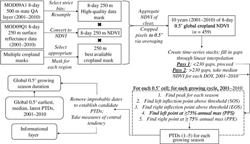
The processing steps and the general logic behind the phenological transition dates extraction algorithm are outlined in Figure 1. We begin with a description of the generation of the growing season calendars (Sections 2.1–2.2), followed by a discussion of the PTDs in the context of known cropland phenology in the CONUS (Section 3.1). This analysis is furthered by a quantitative comparison against usual planting and harvest dates for corn and soy in the US Corn/Soy Belt (USDA-NASS 1997; Section 3.l), and the PTDs are analysed for their sensitivity to interannual and regional variability in cropland phenology (Section 3.1.1). This is followed by a discussion of growing season duration (3.2), as well as peak period timing and duration (3.3), which is accompanied by a preliminary analysis of the impact of multiple crop presence on PTD detection (3.4).

Figure 1. A flowchart depicting the pre-processing and data preparation steps, the basic logic of the PTD extraction algorithm, as well as the steps leading to the generation of the final data products. Intermediate data products and steps are in solid rectangles, actions are connecting arrows accompanied by italicised text, and final data products are in soft-cornered rectangles.

2.1. Data pre-processing and preparation

Ten years (2001–2010) of global, 250 m 8-day surface reflectance data (MOD09Q1) were converted to normalized difference vegetation index (NDVI; Rouse et al. 1974), and then were adjusted through the application of strict quality assessment (QA) bits from the state QA layer for MOD09A1 (Vermote, El Saleous, and Justice 2002) which had been resampled from 500 m to 250 m. The data were not, however, adjusted for the effects of bidirectional reflectance. Data converted to NDVI have been shown to be less impacted by variable view and azimuth angles throughout the growing season than the Enhanced Vegetation Index (EVI), or red and near-infrared channel data alone, at least partially justifying the lack of bidirectional reflectance distribution function (BRDF) adjustment (Bréon and Vermote 2012; Sims et al. 2011).

Before aggregating from 250 m to 0.5° to create a cropland-specific NDVI, cropland pixels needed to be identified. A suite of cropland masks and land cover products were used to do so, all produced in 2001 or more recently, with preference given to those products which were percentage or probability products. For example, in the CONUS, the cropland layer from the National Land Cover Database (NLCD-2001; Homer et al. 2007) was used by resampling from crop/non-crop values at 30–250 m, with only those 250 m pixels which were ≥80% cropped being aggregated to 0.5° through averaging. Due to some spatial gaps left after the analysis using NLCD-2001, an additional ‘background’ layer was generated from Pittman et al.'s (2010) discrete cropland mask to generate more complete coverage. The cropland mask used for each 0.5° grid cell is identified in a supplementary informational layer.

Each resulting time series of these 0.5° 8-day QA-adjusted cropland NDVI images had a number of temporal gaps due to the stringent QA requirements. These gaps as well as those values which dropped below the mean annual minimum NDVI (2001–2010) for that grid cell (perhaps due to errors in cloud screening; Huete et al. 2002) were replaced using linear interpolation, so as not to distort the annual ranges of NDVI. This gap-filled time series of 0.5° cropland NDVI was run through the PTD extraction algorithm during Pass 1. Those 0.5° grid cells for which >50% (n = 230) of the 10-year time series was missing (largely due to chronic cloud cover) were initially not processed for PTDs in Pass 1. A subsequent pass (Pass 2 in Figure 1) at processing was carried out for these areas in which a single year-long time series was constructed out of the median NDVI value for each compiling day of the year (DOY) over 10 years and then processed for PTDs. This latter pass yielded useable dates for many areas, but still left some persistently cloudy areas (e.g. central Africa, parts of Southeast Asia) without PTDs.

2.2. Extracting phenological transition dates from time series NDVI

NDVI is a metric which has long been used as an indicator of above ground green biomass (AGB), vigor, stress, photosynthetic capacity, and leaf area index (LAI), and as a proxy for vegetation health (Baret and Guyot 1991; Jackson 1986; Rouse et al. 1974; Sellers 1985; Tucker 1979; Tucker et al. 1981; Wiegand and Richardson 1990). The Moderate Imaging Spectroradiaometer (MODIS), with improved radiometric and geometric properties and atmospheric correction, has provided higher quality data, which have proven useful for land biophysical applications (Justice et al. 1998; Vermote, El Saleous, and Justice 2002; Wardlow, Kastens, and Egbert 2006). The NDVI was chosen because it has been shown to be suitable for studying phenology in the CONUS (Goward, Tucker, and Dye 1985), and involves only the two MODIS bands which have 250 m (231.65635 m, precisely) resolution, whereas the Enhanced Vegetation Index (EVI) would require the incorporation of coarser 500 m data (Huete et al. 2002), in addition to being less resistant to BRDF effects (Sims et al. 2011). In areas where croplands are small and fragmented and the agricultural landscape is heterogeneous, the use of finer resolution data can potentially reduce the inclusion of non-cropped surfaces (Townshend and Justice 1988; Duveiller and Defourny 2010; Duveiller, Baret, and Defourny 2011; Pittman et al. 2010; Wardlow, Egbert, and Kastens 2007), justifying the choice of 250 m over 500 m observations.

Planting and harvest are processes, which are not easily detected by moderate-to-coarse sensors such as the MODIS instruments, as planting does not result in instantaneous crop-specific above-ground biomass (AGB) generation, and harvesting often leaves a large volume of AGB present, continuing to influence reflectance for some time after the end of the cropping season (B. C. Reed et al. 1994; Wardlow, Kastens, and Egbert 2006). Furthermore, soil background and in some cases non-crop vegetation can influence the signal in advance of and immediately after planting (Galford et al. 2008; Wardlow, Kastens, and Egbert 2006). For these reasons, this analysis identifies a series of PTDs (Table 1) that can be related to cropping practices: first, the start of growing season (SOS) has been identified as the point when an up-sloping NDVI surpasses a certain threshold (for background vegetation) in a period preceding an annual maximum (peak) NDVI. This point describes the onset of photosynthetic activity, also known as the greenup (Zhang et al., 2003), and marks the beginning of a crucial time for monitoring crop development (Becker-Reshef et al. 2010a). Second, the end of growing season (EOS) is considered the point at which a down-sloping NDVI drops below a certain threshold in the period following the annual peak, marking the end of senescence and the termination of photosynthetic activity for the crops (Zhang et al. 2003). The thresholds used in detection of SOS and EOS were determined through an iterative process and were instituted largely to avoid the detection of volunteer weeds, which precede the green-up of actual crops and would bias the SOS earlier, an issue which is likely to be more impactful in areas with high precipitation where tilling is not used (Galford et al. 2008; Wardlow, Kastens, and Egbert 2006). Finally, the peak timing and duration have been identified as the period during which NDVI is ≥75% of its annual range falling around the apparent NDVI maximum. This ‘peak’ metric is unique to satellite data, with Zhang et al. (2003) having described a conceptually similar period (for all vegetated surfaces, not just crops) as representative of the period between the onset of green leaf maximum for a vegetated surface (peak period start; PPS), and the onset of senescence and subsequent rapid decline of photosynthetic activity (peak period end; PPE). Therefore, SOS and EOS dates span the entire active growing season, and are rough estimators of planting and harvest, with SOS theoretically occurring after the actual planting, while the peak period bounds the portion of the growing season during which the LAI maximum will occur (Zhang et al. 2003).

Multiple methods have been established in the literature for extracting phenological information from temporal curves of NDVI, primarily using thresholds, inflection points, largest increases/decreases, and divergence from an established trend (e.g. Jönsson and Eklundh 2004). Lloyd (1990), Fischer (1994), and White, Thornton, and Running (1997) all used NDVI thresholding approaches to detect seasonal changes in vegetation, wherein a certain NDVI value is assumed as indicative of a change in vegetation stage, while Moulin et al. (1997) identified as beginning, peak, and end of season the sign changes (inflection points) of the first derivative of the NDVI curve. The methodology adopted for this study can be described as a combination of the application of thresholds with detection of inflection points.

It should be emphasized and reiterated that there is an additional difference between what this research aims to detect (the timing of the agricultural growing season for the purpose of understanding the necessary periods of satellite imagery acquisition), and what traditional crop calendars are describing (the timing of a single crop's planting, vegetative, maturing, flowering, silking, doughing, transplanting etc. stages, and harvesting). In all but perhaps the most homogenous cropping landscapes, the 0.5° grid cell is comprised of more than one single crop type often with different phenologies, particularly if there is a mix of winter and spring/summer crops (Ozdogan 2010; Pan et al. 2012). The problem of subpixel heterogeneity in cultivated areas is frequently encountered in crop type mapping and monitoring (Duveiller and Defourny 2010; Lobell and Asner 2004; Ozdogan and Woodcock 2006; Pax-Lenney and Woodcock 1997), and it is expected that the mixing of these signals will similarly impact the apparent timing of these different PTDs, with the extent to which these signals are mixed, changing the extent to which the PTDs deviate from existing crop calendars. That is, a 0.5° cell for which the majority of the 250 m cropped pixels’ crop type is corn will yield PTDs closer to that of corn's crop calendar than will an area that is equal parts corn and winter wheat (Pan et al. 2012). A test of the effects of mixing known winter and spring crops’ signals (from USDA-NASS Cropland Data Layer 2006, 2007) in different proportions on PTD determination has been performed for a few sites in Kansas and Missouri to give preliminary insight into this complex topic (see Section 3.4).

2.3. Growing season calendar compilation

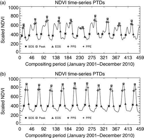
For each 0.5° grid cell, the PTD detection algorithm yielded up to 10 viable SOS and EOS dates, as well as 10 viable PPS and PPE (Figure 2(a) and 2(b)). When defining the agricultural growing season for the purpose of satellite imagery acquisition, cost and operational constraints are critically important and as such the exclusion of even potentially spurious dates is crucial from a strategic standpoint. Outlier removal is challenging and problematic in very dynamic cropping systems with high interannual variability, but is justifiable in the context of developing an image acquisition strategy, where imaging resource and cost constraints must be considered. Accordingly, measures of central tendency were taken to identify and remove dates which fell more than one median absolute deviation from the median. From this ‘cleaned-up’ set of PTD candidates, the earliest, median, and latest SOS, and EOS dates were extracted for each 0.5° grid cell. Two separate growing season duration metrics were calculated: first, the median observed growing season duration from a single season was taken (i.e. each season's detections were analysed separately); and secondly, the number of days between the earliest SOS and the latest EOS date was taken, regardless of whether those observations were from the same season, in order to give an idea of the maximum possible period of time for which observations would be necessary. Meanwhile, the median peak period duration within a single season was extracted, and the corresponding PPS and PPE dates were preserved.

Figure 2. Plots of the gap-filled time series of 8-day composites of scaled NDVI (× 1000), 2001–2010 (46 per year × 10 years = 460 values), from which PTDs were detected. (a) NDVI time series from a location in Southern Kansas, providing an example of a winter wheat dominated landscape, with the SOS being detected in the October-November time period, and the EOS being detected in the June–July time period. The algorithm selects the post-dormancy resumption of growth (Miller 1999) of the crop as the peak period, and in 2001 places the SOS in March (contemporaneous with this post-dormancy re-emergence) due to the true SOS taking place in 2000, before the initiation of the time series. (b) NDVI time series from a location in central Indiana, providing an example of a corn/soy mix, with the SOS being detected in April-May, and the EOS being detected in October.

To accompany these GSCs, an informational map layer was stored which tracks for each 0.5° grid cell the use of quality assessment bits, the impacts of cloud cover, the crop mask used, the degree of interpolation (‘gap-filling’) necessary, as well as measures of central tendency for the dates detected for each cell. Both this information layer as well as the dataset itself can be obtained by contacting the first author.

3. Results

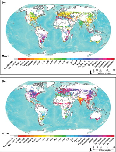
Broadly speaking, the agricultural growing season spans the spring to fall period for northern and southern hemispheres, with notable exceptions for areas of known winter crop (e.g. wheat) cultivation in Australia, the southern Plains/Pacific Northwest of the US, and in areas of southern Europe (Figure 3(a) and 3(b)). For summer/spring crop cultivating areas, we find that the PTDs follow broad patterns of climate limitation, with later SOS and earlier EOS for areas which are further inland (continental climate), more arid (dryer), and/or further from the Equator (lower winter temperatures). Other factors, such as ability to irrigate, selection of seed varieties, and farmer decision making are likely implicated in these regional variations, but analysis of these factors is outside the scope of this paper.

Figure 3. The global median, (a) SOS date, and (b) EOS date, as observed between 2001 and 2010. The PTDs are natively at 0.5°, but the inclusions of even a single 250 m cropped pixel in any of those half-degree grid cells would lead to a large overestimation of cropland extent. In this global view, a cropland indicator mask (GLAM-UMD; unpublished) at 0.05° has been overlaid to provide a more realistic extent of cropland area. Some grid cells (shown in grey) had no detection over 2001–2010, despite having at least some cropland present. If greater than 50% of a grid cell's time series was missing due to insufficient observations (cloud cover presence, low quality observation) that grid was not processed for PTDs.

As discussed above, there are no reliable data against which the global product can be compared. For this reason, these GSCs are in the process of being vetted by regional and national experts within the GEO Agriculture Community of Practice, whose evaluations of the product's accuracy and suggested changes will be in ingested into the final product. Preliminary discussion with experts in areas of Australia, Canada, Argentina, Uruguay, Ukraine, and Russia show that the time periods encapsulated by these GSCs are indeed representative of the periods during which satellite imagery are necessary for their respective areas. For the CONUS, however, this paper presents a comparison of GSC dates against crop calendar dates for a few states in the US Corn Belt from Sacks et al. (2010) digitization of USDA-NASS (1997). Additionally, state-level crop progress data (each state's crop's planting, emergence, and harvesting progress) from USDA-NASS from 2001 to 2010 are compared with each individual year's PTDs to illustrate the GSCs sensitivity to interannual variability.

3.1. Geographical patterns of PTDs observed in the CONUS

Including small contributions from Alaska and Hawaii, an average of 98.9 million hectares were harvested in the USA each year between 2001 and 2010, including those areas for which there were multiple crop rotations and for which each harvest's area was counted. More than 80% of total area harvested is accounted for by three crops: maize (30.9%), soybeans (29.8%), and wheat (both winter & spring varieties, 20.4%), the remainder being largely composed of seed cotton (4.7%), sorghum (2.7%), barley (1.5%), and rice (1.3%; FAOSTAT 2012). A majority of the cultivation is spring and summer crops, although winter wheat and barley are commonly cultivated in the southern half of the CONUS, with much of the west coast states cultivating specialty crops throughout the year (USDA-NASS 1997, 2010).

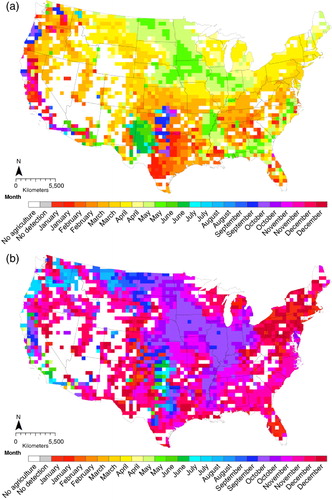
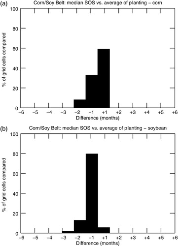
As is expected, the GSCs show that much of the US is dominated by spring and summer crop cultivation, with clear winter crop dominated cultivation in the southern Plains states (Texas, Oklahoma, Kansas), as well as in some portions of the Pacific States, where SOS dates come between August and December (Figure 4(a) and 4(b)). The major corn and soybean producing states are well-characterized with the earliest SOS dates falling generally in April to May and the median SOS dates falling predominately in late May. Meanwhile, the median EOS dates fall in late-September and the latest EOS season dates fall from October to November, which align well with planting ranges (April–May) and harvest ranges (September–November) articulated by USDA-NASS (1997, 2010). In Illinois, Iowa, and Indiana, corn is planted 2–3 weeks before and harvested 1–2 weeks after soybeans. It is expected, then, that SOS dates – which by accounting for multiple crops on the landscape and by approximating emergence are expected to come a few weeks after planting – will fall after corn planting and right around soy planting. Meanwhile, EOS is a rough approximation of harvest without a specified direction of disagreement, and thus EOS should fall sometime around soybean harvest and just before corn harvest. Both of these expectations are represented in the GSCs, as shown through comparison with USDA-NASS's (1997) average planting and harvest dates for corn (Figure 5(a) and 5(d)) and soybean (Figure 5(b)–(c)), respectively, for Illinois, Indiana and Iowa (n = 161 0.5° cells). Each of these states produces large quantities of corn and soybean relative to other crops, meaning that their relative homogeneity makes them an appropriate area for comparing single crop calendars with the GSCs.

Figure 4. For the CONUS, the median (a) SOS date, and (b) EOS date, as observed between 2001 and 2010. The GSCs are shown at their native resolution (0.5°) without any post-processing application of a finer scale cropland mask to account for true cropland extent estimation (as in Figure 3(a) and 3(b)).

Figure 5. Histograms of GSCs minus Sacks et al. (2010)/USDA (1997) planting or harvest dates for a part of the Corn Belt (Illinois, Indiana, Iowa), where a negative value indicates an earlier GSC and a positive value indicates a later GSC relative to planting or harvest dates. Very few 0.5° grid cells agreed perfectly, and so were placed in the +1 month category if they existed. Clockwise from top left: (a) median SOS date minus average corn planting date; (b) median SOS date minus average soybean planting date; (c) median EOS minus average soybean harvesting date; (d) median EOS minus average corn harvesting date.

Beyond the major corn and soy producing states of the CONUS, there also exist three major areas of cotton cultivation – Western Texas (TX), along the Mississippi River (Louisiana, Arkansas, and Mississippi), and in the southeast (Southern Georgia and Eastern Carolinas). In TX, the most active planting takes place in May-June, with the most active harvest period taking place during November, while in both the southeast and the states along the Mississippi River, planting takes place during April-May with harvest occurring in October-November in the former case, and primarily October in the latter case (USDA-NASS 1997). All of these dates are accurately represented by the GSCs.

In California (CA), the existence of a climate that is amenable to year-round cultivation leads to a more variable suite of suitable crops, including a wide variety of specialty crops. According to USDA-NASS (1997), in CA planting spans the entire year, while harvesting spans from 1 April (sugarbeets) until 10 December (sugarbeets), and this is not to mention specialty crops (e.g. grapes, berries) growing in the state. The GSCs reflect these dynamics, even detecting rice cultivation in the Sacramento River Valley, spanning from May until October. With respect to the northeast, the majority of cultivation in that area is actually alfalfa hay (year round cultivation) with a small area of corn production in New York, for which the corresponding USDA-NASS (1997, 2010) crop calendar dates (April/May to October/November) are closely approximated in the GSCs, April/May to November/December. From an Earth observations perspective, this area is not a high priority due to its low production of food crops, and therefore, does not merit further investigation for the purpose of this study.

3.1.1. Sensitivity of GSCs to interannual and regional phenological variations

The USDA-NASS's Usual Planting and Harvesting Dates for US Field Crops (1997, 2010) referenced in this paper, give ranges of observed planting and harvest dates for entire states for a given crop, aggregating information from multiple geographic locations and multiple years. These roughly decadal releases are based off of yearly crop progress data on state-wide percentage of crop type that have been planted, emerged, and harvested. This means that for a given year, a single set of progress information exists for an entire state despite the percentage planted/emerged/harvested values themselves essentially being representations of aggregated geographic variations in planting, emergence, and harvest timing across a state (that is to say, the progress data indicates on a certain day of the year, 20% of the state has been planted, but there is no spatial information on which areas that 20% occupies). In contrast, the GSCs are at a finer resolution (0.5°), meaning that they avoid this geographic aggregation and provide insight into within-state variations in phenological transitions.

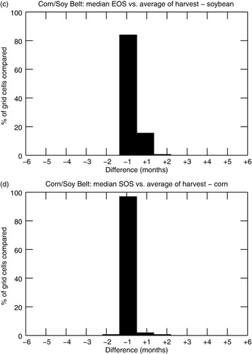
For Illinois, Indiana, and Iowa, we have taken the days of year which correspond with five thresholds (0–20%, 20–40%, 40–60%, 60–80%, and 80–100%) of area planted and area emerged corn progress data for each year 2001–2010 (USDA-NASS Quick Stats 2013), and correlated them with SOS dates to try to determine whether the GSC PTDs are sensitive to interannual variability in cropping dynamics. The same approach has been taken with area harvested thresholds and EOS dates. Because of the geographic aggregation present in the state-level corn progress data, it is expected that certain percent planted/emerged/harvested thresholds will produce better correlations with SOS/EOS dates. Figure 6(a)–(c) show the maximum correlation value (0–1), as well as that maximum value's corresponding crop progress threshold. Keeping in mind that this is a correlation for only corn, and not soybeans or winter wheat or any other crop that may exist in these states, the GSC PTD algorithm is fairly sensitive to interannual variability in cropping dynamics, particularly with percent emerged and percent harvested emergence and harvest. This not only demonstrates that the GSC PTD algorithm is sensitive to interannual variability in cropping dynamics, but also clearly illustrates the utility of this type of finer scale analysis of cropland phenology over previous articulations, particularly in the context of planning fine resolution/small swath satellite image acquisitions.

Figure 6. Maps of yearly GSC 0.5° grid cells correlated with different crop progress percentages from state-level USDA-NASS yearly crop progress data, both sets from 2001 to 2010. On the right is the maximum correlation value from the five crop progress percentage thresholds, and on the left is the crop progress threshold for which that maximum correlation value exists. (a) Yearly percent planted correlated with yearly SOS; (b) yearly percent emerged with yearly SOS; (c) yearly percent harvested with yearly EOS. As expected, SOS has higher correlation with emergence than it does with planting. EOS dates, with their consistently high correlation with harvesting dates, show particular sensitivity to interannual variability in phenology.

3.2. Duration of the agricultural growing season

From an imaging perspective, the duration of the agricultural growing season is important as it indicates the total number of days for which satellite imagery would be needed for agricultural monitoring, with the acknowledgement that not all monitoring applications require imagery throughout the entire growing season. There are several ways to define the duration of the agricultural growing season when there are several years of SOS and EOS PTDs. For example, the maximum possible number of days for which imagery would be required could be taken as the number of days between the earliest SOS and the latest EOS date observed between 2001 and 2010, regardless of whether those dates are from the same growing season or not. This, however, might yield an artificially long growing season due to interannual variability in cultivation practices. Instead, presented here is median growing season duration observed in a single season between 2001 and 2010 (Figure 7).

Figure 7. The median duration of the agricultural growing season (SOS to EOS from the same growing season), 2001–2010. As in Figure 3(a) and 3(b), the GLAM-UMD cropland indicator mask at 0.05° is overlaid the native 0.5° GSCs to more accurately represent cropland extent.

While the agricultural growing seasons range from 96 to 352 days in duration, the mean growing season length for the entire world is 216 days (median = 224 days), which is just over seven months. Generally speaking, areas with cooler winters (e.g. higher latitudes, areas of higher elevation) and/or less precipitation (e.g. the Sahel) have shorter growing season durations, while areas which are characterized by a warmer and wetter climate have longer growing seasons. The shortest growing seasons are found in the Peace River Valley in Canada, as well as in eastern Russia, north of China. While certain winter crop (e.g. wheat) cultivating areas have apparently shortened growing season durations due to the post-dormancy resumption of growing being tagged as the SOS (Section 3.4), this at least highlights the most active period of the AGS for monitoring and is important and new information.

These relationships hold in the CONUS, where growing season durations follow a geographic pattern largely dictated by regional climate, ranging 96–304 days. The mean growing season length for the CONUS is ∼205 days, or just shy of seven months, with 3.0% of the 0.5° grid cells having growing seasons lasting 3–4 months, 12.9% of grid cells lasting 4–5 months, 15.7% lasting 5–6 months, 19.2% lasting 6–7 months, 26.8% lasting 7–8 months, 15.2% lasting 8–9 months, and 7.3% lasting 9–10 months. For Midwestern states characterized by a continental climate and limited by very cold winters, the growing season tends to be shorter (3–6 months), while those areas characterized by a warmer or less variable year-round climate (West Coast and Southern states) tend to have longer growing seasons (up to 10 months). Exceptions to these rules are found in Western Texas and the Arkansas/Mississippi/Louisiana border, each of which are heavy cotton cultivating areas with 4–5 month growing periods (USDA-NASS 1997). Somewhat surprisingly, longer growing seasons are found in the north eastern CONUS, where a distinct seasonality and cold winter would suggest a shorter, climate-limited growing season. In fact, as stated in Section 3.1, the cultivation of alfalfa hay along with some corn is responsible for this seemingly unusual growing season duration (USDA-NASS 1997).

3.3. Peak period timing and duration

The period during which green leaf area is highest is contemporaneous with the NDVI maximum (Zhang et al. 2003). For reasons identified above, it is important to determine the period during which this NDVI maximum is most likely to occur. However, at 0.5° resolution, an area over which many 250 m pixels potentially representing a variety of crop types have been averaged, the relationship between apparent NDVI maximum and individual crop's LAI maximum is perhaps more tenuous as out-of-sync NDVI maxima are blended to form a flatter and broader peak period. To allow for this flattening and broadening effect and encompass a broader period during which the maximum NDVI is likely to occur, the peak period was defined as the period for which NDVI is ≥75% of the annual NDVI range (between the peak period start (PPS) and the peak period end (PPE); Figure 8(a)–(c)). This value – 3/4 maximum – was selected through an iterative process, so as to simply define a period of time just broad enough to likely bound the NDVI maximum. Ten years of PPS and PPE dates were detected, and compiled similar to the SOS/EOS dates (see Section 2.3).

Figure 8. The median (a) peak period start date and, (b) peak period end date as observed between 2001 and 2010, as well as (c) the median peak period duration for that period, which is the number of days between (a) and (b). As in Figures 3(a), 3(b), and 8, the GLAM-UMD cropland indicator mask at 0.05° is overlaid the native 0.5° GSCs to more accurately represent cropland extent.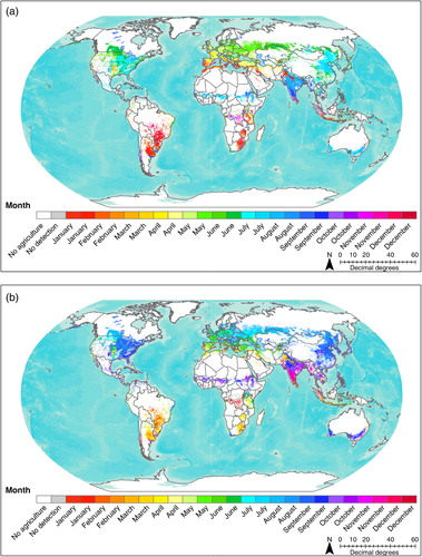

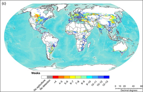
For most of the world, the ≥75% of the annual NDVI range peak period lasts between 4 and 12 weeks, with longer peak periods typically occurring in the same areas that have longer growing season durations and/or that are known to have multiple crops present on the landscape. Within the CONUS, there are two areas with distinctly shorter peak period durations: (1) the major winter wheat cultivation area in Kansas/Oklahoma (KS/OK), and, (2) the Montana (MT) and western North/South Dakotas (ND/SD). In the former case, the shortened peak period corresponds with the steeper, shorter (duration) peak associated with the winter wheat's post-dormancy resumption of growth. In the latter case, MT and western ND cultivate almost solely wheat (spring variety) and spring barley, which have nearly identical calendars (USDA-NASS 1997). In contrast, eastern ND/SD have large areas of sugar beet, corn, and soybean cultivation in addition to wheat (spring in ND, winter and spring in SD) and barley (mostly ND), and accordingly have longer peak period durations, illustrating how multiple crops’ signals, even when somewhat similarly timed, can combine to create a broader, longer apparent peak NDVI period.

In areas for which multiple, distinct cropping cycles, and therefore distinct peaks exist, the peak period approach weakens as the algorithm considers only the dates that surround the annual maximum NDVI rather than allowing for multiple peaks in a year. In the KS/OK area dominated by winter wheat production, the peak period is capturing the winter wheat cultivation's peak; however, there is considerable corn and soy cultivation there as well, and, as discussed in the following Section 3.4, the extent to which the increases in corn/soy NDVI impact the apparent timing of the winter wheat NDVI peak is contingent upon the relative proportions of winter versus spring crops.

3.4. Winter wheat presence and impacts on PTD detection

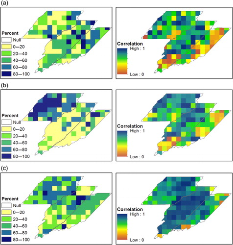
When comparing a corn & soybean only compilation of Sacks et al.'s (2010) digitization of USDA-NASS (1997) usual planting and harvest dates with the GSCs, moving toward areas with a larger winter wheat presence, such as Kansas, Eastern Colorado, Western Nebraska, South Dakota, and Southern Illinois, the GSC SOS dates begin to come before the start of planting dates for corn and soy, which illustrates that winter crop presence causes an earlier SOS detection, although the extent of this impact is contingent upon the ratio of winter to spring/summer crops in an area (Figure 9). In fact, it is not until Southern Kansas, Central Oklahoma, and the Texas/Oklahoma border – where winter wheat becomes the dominant crop – that the GSC PTDs begin to correspond more strongly with known winter wheat calendar dates (September planting, June/July harvesting; USDA-NASS 1997).

Figure 9. The earliest SOS date (2001–2010) minus a corn & soybean-only compilation of the Start of Planting period (based on maximum harvested area fraction, Monfreda, Ramankutty, and Foley (2008)) for the CONUS’ Corn Belt. A negative number indicates an earlier GSC SOS date relative to the start of the planting period, while a positive number indicates a later GSC SOS date versus the start of the planting period.

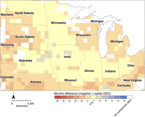
After planting and an initial emergence, winter wheat enters a period of dormancy during winter and resumes growth in early spring (Miller 1999). It is not uncommon that this initial emergence does not produce a sufficiently large increase in NDVI to be detected and classified as a start of season, particularly if within the same 0.5° grid cell there is a large spring/summer crop presence, as the spring/summer crop's contemporaneous NDVI decrease from end of season senescence and harvesting further mutes any NDVI increase. Due to these factors, the GSC's often detect an SOS date for an area with a considerable winter crop presence as late as the end of March, which in reality is the point in time when the crop resumes growth after dormancy. This phenomenon is present in Ukraine and parts of Russia (Figure 3(a)), as well as in certain areas of Kansas, Oklahoma, Colorado, and Missouri, where winter wheat is grown alongside a large quantity of spring/summer crops (primarily corn and soy, though in some cases also sorghum). This phenomenon lends itself to a high level of disagreement between a typical winter wheat planting date in September or October and its associated emergence (SOS) date. While the majority of agricultural monitoring applications only require imagery during the most active part of the growing season (from post-dormancy resumption of growing until end of season), biophysical growth models rely on crop biophysical information throughout the growing season including initial emergence/SOS (e.g. Brisson et al. 1998; Jones et al. 2003), and crop type identification applications rely on observations during the SOS, meaning delayed SOS detections are impactful and require attention.

As a preliminary investigation into the impacts of mixed signals on PTD detection, we have used the USDA-NASS Cropland Data Layers from 2006 to 2007 for the Kansas and Missouri areas, extracting 250 m time series for a handful of adjacent corn, soy, and winter wheat cultivating areas (USDA-NASS Cropland Data Layer 2006, 2007), and processing these ‘pure’ pixel signals for crop-specific PTDs using the same algorithm as for the general agricultural GSCs. In order to better understand how grid cells of varying winter wheat proportion diverge from ‘pure’ wheat pixel's PTDs, these corn, soy, and wheat NDVI values have been added together in different ratios and processed for PTDs to create simulations of the various mixed pixels that can exist. Preliminary results show that the proportions of winter wheat required to result in the detection of a PTD equivalent to that of a ‘pure’ wheat pixel varies for SOS, peak of season (NDVI maximum; POS), as well as EOS. For SOS, the required winter wheat proportion is 33–75%, for POS is 33–50%, and for EOS is 67–85%. Meanwhile, even a small proportion of wheat was capable of changing apparent PTDs by one compositing period (8 days) for corn (SOS: 25–50%; POS: 5–17%; EOS: 7–33%) or soy (SOS: 9–25%; POS: 5–20%; EOS: 5–50%). These findings are from only a small sample of sites and are very preliminary, but serve to suggest that in the context of deriving PTDs, the proportions of crops that make up the unit of analysis do matter and merit further investigation.

4. Discussion, known issues, and future research

The research presented here includes a suite of results that improve our understanding of the agricultural growing season worldwide. First and foremost, it provides a set of GSCs at 0.5°, providing SOS and EOS PTDs detected between 2001 and 2010 from MODIS surface reflectance data. This information enables us to identify the period during which FTM Earth observations for agriculture monitoring are required. Additionally, it identifies those periods of the growing season (e.g. SOS as onset of emergence, peak period as ‘bounding box’ for the NDVI maximum, EOS as approximation of harvesting period) for which imaging is critically important. For the purpose of developing an image acquisition strategy for agriculture monitoring, this study has articulated the timing of necessary image acquisitions for the global agricultural regions, providing the foundation for a continued investigation into the frequency of necessary observations, as well as the necessary spatial and spectral (optical vs. active/microwave) resolutions as inputs to a global agriculture monitoring imaging constellation system.

There remain a few areas for which no viable detection was possible, usually due to persistent cloud cover creating too many gaps in the time series. Tandem efforts exist at the International Rice Research Institute (IRRI) for the production of rice crop calendars. As many of the areas lacking dates are rice cultivating – for example, coastal West Africa and Southeast Asia – this provides a remedy. In fact, for major rice producing areas, these calendars should be substituted regardless, as the highly variable year-to-year sowing dates for rice and year-round cultivation are not adequately accounted for by the PTD detecting algorithm described above.

As discussed above and demonstrated by a preliminary analysis (Section 3.4), the impacts of multiple cropping's mixed signals on PTD detection are present, but their magnitude is not well-understood. In the future, a more in-depth analysis of these impacts for a larger sample of sites would provide insight into the limitations of coarser spatial resolution analyses of croplands in general and phenology in particular.

In addition to farmer decision making and farming systems, climatic variables such as temperature and precipitation are known to impact observed SOS and EOS dates both across regions and between years. An analysis of the relationships between climatic variables and PTDs merits further research, but is beyond the scope of this paper.

While the emphasis of this research is on defining the growing season from the perspective of developing a viable image acquisition strategy for agriculture monitoring in the context of GEOGLAM, the growing season calendar and its associated methodology could be useful as inputs for other applications. This is particularly true if attempts are made to separate out the major crops and move back into the realm of crop-specific growing season calendars, research that would be facilitated by crop-specific masks, which currently do not exist globally at a sufficiently fine resolution. The present resolution (0.5°) was chosen to fall within the swath widths of FTM sensors, but the PTD detection algorithm is suitable for use at any resolution. As the algorithm has been shown to reasonably model known cropland phenology and to account for regional and interannual variability in cropping practices (at least in the Corn Belt of the CONUS), it can and should be applied to crop-specific time series in order to generate fine resolution, spatially explicit crop-specific crop calendars to accompany the general agricultural GSCs presented herein.

Acknowledgements

The authors would like to thank NASA for the support for this research (NNX11AL56H). Additionally, the authors would like to acknowledge Louis Giglio of the University of Maryland, College Park Department of Geographical Sciences for technical guidance, as well as those in the Group on Earth Observations Agricultural Monitoring Community of Practice for their ongoing review of the growing season calendars.

Additional information

Funding

This work was supported by the National Aeronautics and Space Administration [grant number NNX11AL56H].

References

- Allen, Rich, George Hanuschak, and Mike Craig. 2002. History of Remote Sensing for Crop Acreage in USDA's National Agricultural Statistics Service. NASS.
- Baret, Fred, and Gerard Guyot. 1991. “Potentials and Limits of Vegetation Indices for LAI and APAR Assessment.” Remote Sensing of Environment 35 (2): 161–173. doi:10.1016/0034-4257(91)90009-U.
- Bastiaanssen, Wim G. M., David J. Molden, and Ian W. Makin. 2000. “Remote Sensing for Irrigated Agriculture: Examples from Research and Possible Applications.” Agricultural Water Management 46 (2): 137–155. doi:10.1016/S0378-3774(00)00080-9.
- Becker-Reshef, Inbal, Eric Vermote, Mark Lindeman, and Christopher Justice. 2010a. “A Generalized Regression-based Model for Forecasting Winter Wheat Yields in Kansas and Ukraine Using MODIS Data.” Remote Sensing of Environment 114 (6): 1312–1323. doi:10.1016/j.rse.2010.01.010.
- Becker-Reshef, Inbal, Chris Justice, Mark Sullivan, Eric Vermote, Compton Tucker, Assaf Anyamba, Jen Small, Ed Pak, Ed Masuoka, and Jeff Schmaltz. 2010b. “Monitoring Global Croplands with Coarse Resolution Earth Observations: The Global Agriculture Monitoring (GLAM) Project.” Remote Sensing 2 (6): 1589–1609. doi:10.3390/rs2061589.
- Biradar, Chandrashekhar M., and Xiangming Xiao. 2011. “Quantifying the Area and Spatial Distribution of Double- and Triple-cropping Croplands in India with Multi-temporal MODIS Imagery in 2005.” International Journal of Remote Sensing 32 (2): 367–386. doi:10.1080/01431160903464179.
- Boken, Vijendra K., and Carl F. Shaykewich. 2002. “Improving an Operational Wheat Yield Model Using Phenological Phase-based Normalized Difference Vegetation Index.” International Journal of Remote Sensing 23 (20): 4155–4168. doi:10.1080/014311602320567955.
- Bréon, Franccois-Marie, and Eric Vermote. 2012. “Correction of MODIS Surface Reflectance Time Series for BRDF Effects.” Remote Sensing of Environment 125: 1–9. doi:10.1016/j.rse.2012.06.025.
- Brisson, Nadine, Bruno Mary, Dominique Ripoche, Marie Hélène Jeuffroy, Franccoise Ruget, Bernard Nicoullaud, Philippe Gate, Florence Devienne-Barret, Rodrigo Antonioletti, and Carolyne Durr. 1998. “STICS: A Generic Model for the Simulation of Crops and Their Water and Nitrogen Balances. I. Theory and Parameterization Applied to Wheat and Corn.” Agronomie 18 (5–6): 311–346. doi:10.1051/agro:19980501.
- Duveiller, Grégory, Frédéric Baret, and Pierre Defourny. 2011. “Crop Specific Green Area Index Retrieval from MODIS Data at Regional Scale by Controlling Pixel-target Adequacy.” Remote Sensing of Environment 115 (10): 2686–2701. doi:10.1016/j.rse.2011.05.026.
- Duveiller, Grégory, and Pierre Defourny. 2010. “A Conceptual Framework to Define the Spatial Resolution Requirements for Agricultural Monitoring Using Remote Sensing.” Remote Sensing of Environment 114 (11): 2637–2650. doi:10.1016/j.rse.2010.06.001.
- FAOSTAT. 2012. “Agriculture Organization of the United Nations.” Statistical Database.
- Fischer, Alberte. 1994. “A Model for the Seasonal Variations of Vegetation Indices in Coarse Resolution Data and Its Inversion to Extract Crop Parameters.” Remote Sensing of Environment 48 (2): 220–230. doi:10.1016/0034-4257(94)90143-0.
- Galford, Gillian L., John F. Mustard, Jerry Melillo, Aline Gendrin, Carlos C. Cerri, and Carlos E. P. Cerri. 2008. “Wavelet Analysis of MODIS Time Series to Detect Expansion and Intensification of Row-crop Agriculture in Brazil.” Remote Sensing of Environment 112 (2): 576–587. doi:10.1016/j.rse.2007.05.017.
- Goward, Samuel N., Compton J. Tucker, and Dennis G. Dye. 1985. “North American Vegetation Patterns Observed with the NOAA-7 Advanced Very High Resolution Radiometer.” Plant Ecology 64 (1): 3–14. doi:10.1007/BF00033449.
- Homer, Collin, Jon Dewitz, Joyce Fry, Michael Coan, Nazmul Hossain, Charles Larson, Nate Herold, Alexa McKerrow, J. Nick VanDriel, and James Wickham. 2007. “Completion of the 2001 National Land Cover Database for the Counterminous United States.” Photogrammetric Engineering and Remote Sensing 73 (4): 337.
- Huete, A., Kamel Didan, Tomoaki Miura, E. Patricia Rodriguez, Xiang Gao, and Laerte G. Ferreira. 2002. “Overview of the Radiometric and Biophysical Performance of the MODIS Vegetation Indices.” Remote Sensing of Environment 83 (1): 195–213. doi:10.1016/S0034-4257(02)00096-2.
- Jackson, Thomas J. 1986. “Soil Water Modeling and Remote Sensing.” IEEE Transactions on Geoscience and Remote Sensing GE-24 (1): 37–46. doi:10.1109/TGRS.1986.289586.
- Jones, James W., Gerrit Hoogenboom, Cheryl H. Porter, Ken J. Boote, William D. Batchelor, Tony Hunt, Paul W. Wilkens, Upendra Singh, Arjan J. Gijsman, and Joe T. Ritchie. 2003. “The DSSAT Cropping System Model.” European Journal of Agronomy 18 (3): 235–265. doi:10.1016/S1161-0301(02)00107-7.
- Jönsson, Per, and Lars Eklundh. 2004. “TIMESAT—A Program for Analyzing Time-series of Satellite Sensor Data.” Computers & Geosciences 30 (8): 833–845. doi:10.1016/j.cageo.2004.05.006.
- Justice, Christopher O., and Inbal Becker-Reshef. 2007. “Report from the Workshop on Developing a Strategy for Global Agricultural Monitoring in the Framework of Group on Earth Observations (GEO).” UN FAO, July.
- Justice, Christopher O., Eric Vermote, John R. G. Townshend, Ruth DeFries, David P. Roy, Dorothy K. Hall, Vincent V. Salomonson, et al. 1998. “The Moderate Resolution Imaging Spectroradiometer (MODIS): Land Remote Sensing for Global Change Research.” IEEE Transactions on Geoscience and Remote Sensing 36 (4): 1228–1249. doi:10.1109/36.701075.
- Lloyd, Daniel. 1990. “A Phenological Classification of Terrestrial Vegetation Cover Using Shortwave Vegetation Index Imagery.” Remote Sensing 11 (12): 2269–2279. doi:10.1080/01431169008955174.
- Lobell, David B., and Gregory P. Asner. 2004. “Cropland Distributions from Temporal Unmixing of MODIS Data.” Remote Sensing of Environment 93 (3): 412–422. doi:10.1016/j.rse.2004.08.002.
- MacDonald, Robert B., and Forrest G. Hall. 1980. “Global Crop Forecasting.” Science 208: 670–679. doi:10.1126/science.208.4445.670.
- Miller, Travis D. 1999. “Growth Stages of Wheat: Identification and Understanding Improve Crop Management. Texas Agricultural Extension Service, the Texas A&M University System”. SCS-1999-16.
- Monfreda, Chad, Navin Ramankutty, and Jonathan A. Foley. 2008. “Farming the Planet: 2. Geographic Distribution of Crop Areas, Yields, Physiological Types, and Net Primary Production in the Year 2000.” Global Biogeochemical Cycles 22 (1): GB1022. doi:10.1029/2007GB002947.
- Moulin, Sophie, Laurent Kergoat, Nicolas Viovy, and Gerard Dedieu. 1997. “Global-scale Assessment of Vegetation Phenology Using NOAA/AVHRR Satellite Measurements.” Journal of Climate 10 (6): 1154–1170. doi:10.1175/1520-0442(1997)010%3C1154:GSAOVP%3E2.0.CO;2.
- Ozdogan, Mutlu. 2010. “The Spatial Distribution of Crop Types from MODIS Data: Temporal Unmixing Using Independent Component Analysis.” Remote Sensing of Environment 114 (6): 1190–1204. doi:10.1016/j.rse.2010.01.006.
- Ozdogan, Mutlu, and Curtis E. Woodcock. 2006. “Resolution Dependent Errors in Remote Sensing of Cultivated Areas.” Remote Sensing of Environment 103 (2): 203–217. doi:10.1016/j.rse.2006.04.004.
- Pan, Yaozhong, Le Li, Jinshui Zhang, Shunlin Liang, Xiufang Zhu, and Damien Sulla-Menashe. 2012. “Winter Wheat Area Estimation from MODIS-EVI Time Series Data Using the Crop Proportion Phenology Index.” Remote Sensing of Environment 119: 232–242. doi:10.1016/j.rse.2011.10.011.
- Pax-Lenney, Mary, and Curtis E. Woodcock. 1997. “The Effect of Spatial Resolution on the Ability to Monitor the Status of Agricultural Lands.” Remote Sensing of Environment 61 (2): 210–220. doi:10.1016/S0034-4257(97)00003-5.
- Pittman, Kyle, Matthew C. Hansen, Inbal Becker-Reshef, Peter V. Potapov, and Christopher O. Justice. 2010. “Estimating Global Cropland Extent with Multi-year MODIS Data.” Remote Sensing 2 (7): 1844–1863. doi:10.3390/rs2071844.
- Portmann, Felix T., Stefan Siebert, and Petra Döll. 2010. “MIRCA2000—Global Monthly Irrigated and Rainfed Crop Areas Around the Year 2000: A New High-resolution Data Set for Agricultural and Hydrological Modeling.” Global Biogeochemical Cycles 24 (1): GB1011. doi:10.1029/2008GB003435.
- Reed, Bradley C., Jesslyn F. Brown, Darre VanderZee, Thomas R. Loveland, James W. Merchant, and Donald O. Ohlen. 1994. “Variability of Land Cover Phenology in the United States.” Journal of Vegetation Science 5: 703–714. doi:10.2307/3235884.
- Reed, Bradley C., Mark D. Schwartz, and Xiangming Xiao. 2009. “Remote Sensing Phenology.” Phenology of Ecosystem Processes 231–246. doi:10.1007/978-1-4419-0026-5_10.
- Rouse, John W., Robert H. Haas, John A. Schell, Donald W. Deering, and James C. Harlan. 1974. Monitoring the Vernal Advancement and Retrogradation (Greenwave Effect) of Natural Vegetation. Remote Sensing Center, College Station, TX: Texas A & M University. http://library.wur.nl/WebQuery/clc/154154.
- Sacks, William J., Delphine Deryng, Jonathan A. Foley, and Navin Ramankutty. 2010. “Crop Planting Dates: An Analysis of Global Patterns.” Global Ecology and Biogeography 19 (5): 607–620. doi:10.1111/j.1466-8238.2010.00551.x.
- Sakamoto, Toshihiro, Brian D. Wardlow, Anatoly A. Gitelson, Shashi B. Verma, Andrew E. Suyker, and Timothy J. Arkebauer. 2010. “A Two-step Filtering Approach for Detecting Maize and Soybean Phenology with Time-series MODIS Data.” Remote Sensing of Environment 114 (10): 2146–2159. doi:10.1016/j.rse.2010.04.019.
- Sakamoto, Toshihiro, Masayuki Yokozawa, Hitoshi Toritani, Michio Shibayama, Naoki Ishitsuka, and Hiroyuki Ohno. 2005. “A Crop Phenology Detection Method Using Time-series MODIS Data.” Remote Sensing of Environment 96 (3): 366–374. doi:10.1016/j.rse.2005.03.008.
- Sellers, Piers J. 1985. “Canopy Reflectance, Photosynthesis and Transpiration.” International Journal of Remote Sensing 6 (8): 1335–1372. doi:10.1080/01431168508948283.
- Sims, Daniel A., Abdullah F. Rahman, Eric F. Vermote, and Zuoning Jiang. 2011. “Seasonal and Inter-annual Variation in View Angle Effects on MODIS Vegetation Indices at Three Forest Sites.” Remote Sensing of Environment 115 (12): 3112–3120. doi:10.1016/j.rse.2011.06.018.
- Singh Parihar, Jai, Chris Justice, Jo Soares, Olivier Leo, Pascal Kosuth, Ian Jarvis, Derrick Williams, Wu Bingfang, John Latham, and Inbal Becker-Reshef. 2012. “GEO-GLAM: A GEOSS-G20 Initiative on Global Agricultural Monitoring.” 39th COSPAR Scientific Assembly, Mysore, India, July 14–22, 2012. Abstract D2.2-9-12, P.1451, 39:1451. http://adsabs.harvard.edu/abs/2012cosp…39.1451S.
- Stehfest, Elke, Maik Heistermann, Joerg A. Priess, Dennis S. Ojima, and Joseph Alcamo. 2007. “Simulation of Global Crop Production with the Ecosystem Model DayCent.” Ecological Modelling 209 (2–4): 203–219. doi:10.1016/j.ecolmodel.2007.06.028.
- Steven, Michael D. 1993. “Satellite Remote Sensing for Agricultural Management: Opportunities and Logistic Constraints.” ISPRS Journal of Photogrammetry and Remote Sensing 48 (4): 29–34. doi:10.1016/0924-2716(93)90029-M.
- Townshend, John R. G., and Christopher O. Justice. 1988. “Selecting the Spatial Resolution of Satellite Sensors Required for Global Monitoring of Land Transformations.” International Journal of Remote Sensing 9 (2): 187–236. doi:10.1080/01431168808954847.
- Tucker, Compton J. 1979. “Red and Photographic Infrared Linear Combinations for Monitoring Vegetation.” Remote Sensing of Environment 8 (2): 127–150. doi:10.1016/0034-4257(79)90013-0.
- Tucker, Compton J., Brent N. Holben, James H. Elgin, and James E. McMurtrey. 1981. “Remote Sensing of Total Dry-matter Accumulation in Winter Wheat.” Remote Sensing of Environment 11: 171–189. doi:10.1016/0034-4257(81)90018-3.
- USDA-NASS. 1997. “Harvesting Dates for US Field Crops.” US Department of Agriculture National Agricultural Statistics Service.
- USDA-NASS. 2010. Usual Planting and Harvesting Dates for US Field Crops.
- USDA-NASS Cropland Data Layer. 2006. Published Crop Specific Data Layer [Online]. Washington, DC: USDA NASS. Accessed March 4, 2013. http://nassgeodata.gmu.edu/CropScape/.
- USDA-NASS Cropland Data Layer. 2007. Published Crop Specific Data Layer [Online]. Washington, DC: USDA NASS. Accessed March 4, 2013. http://nassgeodata.gmu.edu/CropScape/.
- USDA-NASS Quick Stats. 2013. Crop Progress and Condition, 2001–2010 [Online]. Washington, DC USDA-NASS. Accessed August 16, 2013. http://www.nass.usda.gov/Charts_and_Maps/Crop_Progress_&_Condition/.
- Vermote, Eric F., Nazmi Z. El Saleous, and Christopher O. Justice. 2002. “Atmospheric Correction of MODIS Data in the Visible to Middle Infrared: First Results.” Remote Sensing of Environment 83 (1): 97–111. doi:10.1016/S0034-4257(02)00089-5.
- Wardlow, Brian D., and Stephen L. Egbert. 2008. “Large-area Crop Mapping Using Time-series MODIS 250 m NDVI Data: An Assessment for the U.S. Central Great Plains.” Remote Sensing of Environment 112 (3): 1096–1116. doi:10.1016/j.rse.2007.07.019.
- Wardlow, Brian D., Stephen L. Egbert, and Jude H. Kastens. 2007. “Analysis of Time-series MODIS 250 m Vegetation Index Data for Crop Classification in the US Central Great Plains.” Remote Sensing of Environment 108 (3): 290–310. doi:10.1016/j.rse.2006.11.021
- Wardlow, Brian D., Jude H. Kastens, and Stephen L. Egbert. 2006. “Using USDA Crop Progress Data for the Evaluation of Greenup Onset Date Calculated from MODIS 250-meter Data.” Photogrammetric Engineering and Remote Sensing 72 (11): 1225–1234. doi:10.14358/PERS.72.11.1225.
- White, Michael A., Peter E. Thornton, and Steven W. Running. 1997. “A Continental Phenology Model for Monitoring Vegetation Responses to Interannual Climatic Variability.” Global Biogeochemical Cycles 11 (2): 217–234. doi:10.1029/97GB00330.
- Wiegand, Craig L., and Arthur J. Richardson. 1990. “Use of Spectral Vegetation Indices to Infer Leaf Area, Evapotranspiration and Yield: I. Rationale.” Agronomy Journal 82 (3): 623–629. doi:10.2134/agronj1990.00021962008200030037x.
- Xiao, Xiangming, Stephen Boles, Jiyuan Liu, Dafang Zhuang, Steve Frolking, Changsheng Li, William Salas, and Berrien Moore III. 2005. “Mapping Paddy Rice Agriculture in Southern China Using Multi-temporal MODIS Images.” Remote Sensing of Environment 95 (4): 480–492. doi:10.1016/j.rse.2004.12.009.
- Zhang, Xiaoyang, Mark A. Friedl, Crystal B. Schaaf, Alan H. Strahler, John CF Hodges, Feng Gao, Bradley C. Reed, and Alfredo Huete. 2003. “Monitoring Vegetation Phenology Using MODIS.” Remote Sensing of Environment 84 (3): 471–475. doi:doi:10.1016/S0034-4257(02)00135-9.