Prevalence of the terrain reversal effect in satellite imagery

Abstract

The terrain reversal effect is a perceptual phenomenon which causes an illusion in various 3D geographic visualizations where landforms appear inverted, e.g. we perceive valleys as ridges and vice versa. Given that such displays are important for spatio-visual analysis, this illusion can lead to critical mistakes in interpreting the terrain. However, it is currently undocumented how commonly this effect is experienced. In this paper, we study the prevalence of the terrain reversal effect in satellite imagery through a two-stage online user experiment. The experiment was conducted with the participation of a diverse and relatively large population (n = 535). Participants were asked to identify landforms (valley or ridge?) or judge a 3D spatial relationship (is A higher than B?). When the images were rotated by 180°, the results were reversed. In a control task with ‘illusion-free’ original images, people were successful in identifying landforms, yet a very strong illusion occurred when these images were rotated 180°. Our findings demonstrate that the illusion is acutely present; thus, we need a better understanding of the problem and its solutions. Additionally, the results caution us that in an interactive environment where people can rotate the display, we might be introducing a severe perceptual problem.

Keywords:

• terrain reversal
• relief inversion
• false topographic perception phenomenon
• photo interpretation
• visual illusion
• user study

Introduction and background

Perceptual issues, including optical illusions, have been a topic in visualization research for decades (e.g. Wood 1968; Arnheim 1976; Gilmartin 1981; Cleveland 1983; Pinna and Mariotti 2006). This study assesses the prevalence of a particular optical illusion in geovisualization displays. In this paper, we present results from a two-stage online user experiment concerned with a widely known but poorly understood phenomenon about depth perception in geographic visualizations, commonly referred to as the relief inversion effect (e.g. Imhof 1967; Bernabé-Poveda, Manso-Callejo, and Ballari et al. 2005; Patterson 2013). This phenomenon has been termed the terrain reversal effect (Zhou, Zhang, and Gao 2006; Bernabé-Poveda, Sánchez-Ortega, and Çöltekin 2011), relief inversion fallacy (Kettunen and Sarjakoski 2009), or false topographic perception phenomenon (Saraf et al. 1996). The term relief inversion is also used for physical changes on the surface of the earth, e.g. as a result of an earthquake (e.g. Amit et al. 1999), as a geomorphic process (Pain, Clarke, and Thomas 2007; Pain and Clarke 2009) or as a component of landscape evolution (Pain and Oilier 1995). Throughout this manuscript, we will use the term ‘terrain reversal effect’ because it clearly expresses the experience in geographic contexts and it is nonambiguous.

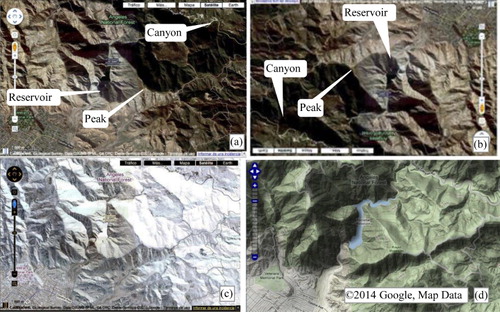
The terrain reversal effect occurs in various geographic visualizations, including artificially lit shaded relief maps and contour maps, as well as in naturally lit imagery, causing the landforms to appear inverted, e.g. valleys are perceived as ridges and vice versa (Figure 1a). While a cartographer can control the artificial lighting fairly easily in shaded relief maps, addressing the issues around natural lighting is often much more complicated. However, satellite images and aerial photographs are commonly used for everyday geographic tasks (e.g. Boer, Çöltekin, and Clarke 2013), and we dedicate considerable computational resources and bandwidth to be able to use them (e.g. Çöltekin and Reichenbacher 2011). Therefore, it needs to be established if, and how severely, we are susceptible to this illusion when we view satellite images and aerial photographs. For example, perceiving mountains as valleys (and vice versa) can be critically misleading in photo interpretation and similar visuospatial tasks.

Figure 1. (a) Pacoima Reservoir, Los Angeles National Forest, as seen on Google Maps. Rivers appear to follow ridges and the reservoir lake in the middle appears as a crater lake. (b) 180° rotation of the same image (without any other alterations) can remove the illusion. Now rivers are in the valleys and the reservoir lake ‘makes more sense’. (c) A negative of the image (again, without further alteration) also removes the illusion (not rotated). (d) The reference terrain represents the real landforms.

Besides the visual interpretation, Saraf et al. (2007) state that the uncorrected light–shade relationships in such geographic imagery may lead to imperfections in image classification and landform delineation tasks. Further systematic tests are necessary to establish the true extent of the terrain reversal effect in image classification tasks; however, the proposition by Saraf et al. (2007) proposition suggests that the problem may be relevant not only to visual but also to computational tasks. In addition to the geographic visualizations, the terrain reversal effect occurs in extraterrestrial imagery such as the Mars or Moon images (e.g. Saraf et al. 2011; Wu, Li, and Gao 2013).

It appears that rotating the image (Figure 1b) or presenting a negative of it (Figure 1c) inverses the perception; i.e. corrects it in this case but adds the illusion in some other cases. These inversions introduced by straightforward geometric and radiometric processes imply that the viewing angle (as obtained by rotating the image) and the color or light information used in shading (as obtained by creating a negative of the image) are likely to be critical to the correct perception of landforms. This is true also for other forms – in fact shape from shading is an important research topic in overall depth perception that is directly related to terrain reversal effect (e.g. Kleffner and Ramachandran 1992; Howard 2002; Liu and Todd 2004; Prados and Faugeras 2006). Therefore, not surprisingly, the terrain reversal effect is frequently linked to the direction of illumination (e.g. Khang, Koenderink, & Kappers 2006; Bernabé-Poveda, Manso-Callejo, and Ballari 2005). Similarly, in cartography literature, Imhof (1967) observes that ‘obliquely lit model images are prone’ to this optical illusion (Imhof 1967, 173). It is demonstrated in literature that when illuminated from the southeast, a north-oriented relief map or image will produce the terrain reversal effect on the viewer (Imhof 1967; Jenny and Patterson 2007; Patterson 2013). Terrain reversal effect is believed to occur frequently in particular in the northern hemisphere (NH; Saraf et al. 2007; Rudnicki 2005; Toutin 1998). The illusion can be very strong and evidently can be critical in map reading and interpretation.

Despite its seemingly obvious importance, we could not identify any study in the literature that demonstrates the prevalence of the terrain reversal effect, neither in a given set of geographic imagery nor in a population of map users. When there is an illusion, the majority of people are expected to experience it; however, in satellite images, this may not be straightforward mainly because the land-cover information sometimes allows people to interpret the spatial relationships in the image, thus bypassing the perceptual signals that would normally lead to the terrain reversal effect. Establishing the prevalence of the illusion in a population of map users would help us understand whether it is only relevant to a special group or if it is a generalizable phenomenon; thus if it is worthwhile (or even necessary at all) to reflect on developing and applying solutions to correct for this perceptual issue. For similar reasons, it is important to establish what proportion of the visualizations, in particular the naturally lit satellite images, seem to lead to this illusion. In this study, we address these research gaps through a qualitative analysis based on an image survey to obtain preliminary answers to the questions ‘what percentage of the images lead to this illusion?’ and ‘is the illusion more common in the NH than in the southern hemisphere?’ (SH) and a two-stage online user experiment to obtain an answer to ‘what percentage of people experience this illusion?’. The user experiment is the main contribution of this paper.

Methods

As a first step, we conducted a qualitative review of popular online map providers to understand whether the problem occurs commonly among the satellite images found online. Further, we randomly sampled 340 locations using one of these map providers and subjectively assessed how frequently the terrain reversal effect occurs among the sampled imagery (‘image survey’). Following this, we surveyed a total of 535 participants in a two-stage online user experiment to infer the prevalence of the terrain reversal effect among the tested people (‘user survey’). While it was not an original objective in the study, we also conducted an exploratory analysis to identify whether we could observe group differences among our participants based on their background, i.e. by age, gender, education, and expertise.

The main methodological approach in this paper is an online user experiment consisting of two structured questionnaires. These questionnaires were delivered in a between-subject manner (i.e. there were two groups of people; the first group worked with original images while the second group worked with 180°-rotated images). The data from the two questionnaires were statistically analyzed.

Determining the frequency of terrain reversal effect in satellite imagery

The prevalence of the terrain reversal effect can be understood in two ways: How common is it in a population (how many people experience the illusion?), and how common is it in a dataset (how many of the images would lead to such an illusion?).

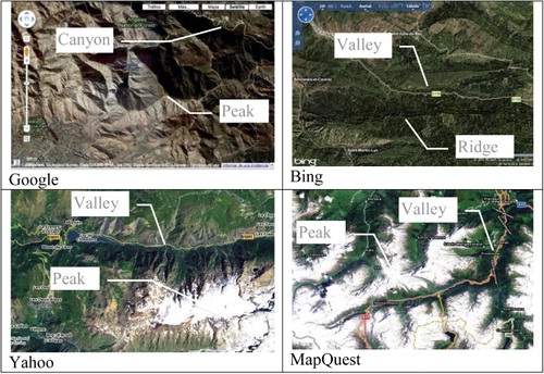
As mentioned earlier, we attempt to answer the first question via a systematic two-stage online user experiment. Regarding the second question, we do not report on a rigorous study but a preliminary subjective analysis. In this preliminary analysis, we first scanned (eyeballing) the satellite view in a selected set of popular map services in random locations; i.e. we visited Google Maps, Bing Maps, Yahoo Maps and MapQuest. The objective here was to determine if we could locate reversed landforms around 10 randomly determined hilly regions. We used land-cover cues (snow/vegetation) and other terrain features (e.g. rivers, which are typically found in valleys) to judge if the illusion was present. This initial assessment was qualitative (one person studying the displays), and its purpose was to decide whether to proceed with the next step. This assessment confirmed that the next steps were well-justified and indicated that the NH locations were more likely to lead to the studied effect in comparison to the SH locations, as previous literature suggested. Following this, to further explore the frequency of the effect in satellite imagery in the NH and SH, we sampled 340 random locations (170 in NH, 170 in SH) on Google Earth. Two people viewed each of these 340 locations, searched for the 3D landforms and reported if they had experienced the illusion based on their judgment of valleys and ridges. To verify the perceptual judgment of the landform, sometimes vegetation and land cover as well as other features such as rivers were used as references, as well as Google Earth's altitude information. We did not introduce a clear spatial or temporal limit. The researcher could ‘give up’ if the terrain was too flat. If (despite hilly terrain) there was no illusion, two participants marked ‘no’ in a spreadsheet, and if they found at least one illusion, they marked ‘yes’. Results from this survey are used as a preliminary indication of the frequency of the terrain reversal effect in satellite imagery in the NH and SH (a more systematic study is currently being conducted).

User experiment

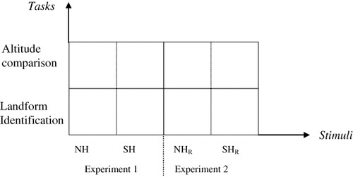
The user experiment consisted of a two-stage online study containing two complementary questionnaires (one questionnaire in each stage) delivered in a between-subject manner (Figure 4). Even though the experimental design was between-subject, the images and questions were essentially repeated in the second survey to ensure consistency; the only thing that varied was the 180° rotation of the images. The questionnaires were advertised via professional email lists as well as via our personal networks to a mixed global audience, and in total 535 participants responded over a period of 6 weeks.

Stimuli and tasks

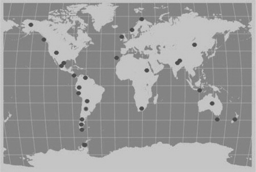
The two questionnaires were designed to include 36 images, distributed all over the globe; more specifically 17 images in the NH, three in the equatorial region, and 16 in the SH (Figure 2). When sampling the images, we took the direction of illumination theory in connection with earth's relative position to sun, some examples in the literature (e.g. Imhof 1967; Saraf et al. 2007), and our perceptual judgment into account. Based on this selection, we expect the NH images to lead to the illusion in the original set, while SH images should not.

Figure 2. Studied locations (where the screenshots were produced). Not all of the 36 locations are indicated in this illustration, as some of them would occlude each other.

At this point, it is important to note that not all imagery from the NH will lead to terrain reversal illusion nor are all the SH images free from it. This distinction (starting with a batch of images which hypothetically should lead to terrain reversal and another batch which should not, based on our own perceptual judgment) allows more control in the experiment. The reason we used samples from the NH and SH is that there appear to be considerably more images in the NH with the terrain reversal illusion.

When selecting the stimuli, we made sure to include a diverse set of landforms to obtain balanced patterns of visual texture. For example, deserts such as Alice Springs, Lhasa, and Port Sudan; wooded areas such as Acapulco and Tasmania; tropical forests such as Puerto Cabello; areas with sudden relief changes such as La Palma, Pichincha, and the Himalayas; or areas with smoother relief changes such as Sonsonate and Loch Loynes were represented in the study. Images were well distributed at different elevation levels to avoid possible bias from the proximity (or remoteness, i.e. the ‘zoom’ levels). We avoided completely flat areas as the terrain reversal effect is much less relevant in such topography, and we qualitatively tried to keep the scene contents comparable in terms of altitude variation in the scene and land-cover cues such as snow, rivers, or vegetation changes. Following the image selection process, screenshots were prepared as static images and later used as stimuli in the two online questionnaires.

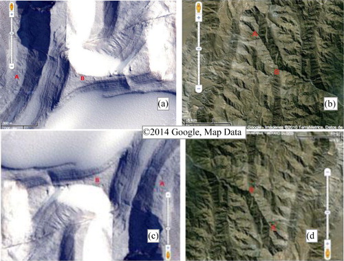
In Experiment 1, participants (n = 253) were presented the original 36 screenshots, as served by the map provider. Participants were asked a 3D landform identification question on the presented satellite image, i.e. whether they see a valley or a ridge. Alternatively, half of the questions were formulated as judgments of 3D spatial relationships, i.e. whether a marked location was higher or lower than another (Figure 3). The alternative answers were presented using a pull-down menu in a binary fashion. Different wording was necessary to correspond with the landforms, and also served as further experimental control, addressing a possible bias in case the wording influences the participants in subtle ways. The landform features were marked with letters. Examples from the stimuli used in the questionnaires and the wording of the tasks can be seen in Figure 3 and its caption.

Figure 3. (a) and (b) are example stimuli from the first questionnaire, and (c) and (d) are examples from the second. Example questions for these stimuli are: (a) and (c) Point A is located in a place higher/lower than B (b) and (d) Line AB looks like a valley/ridge.

In Experiment 2, to avoid a learning effect, another group of participants (n = 282) viewed the same set of images; however, the images were rotated 180°. This experiment measured the effect of the 180° rotation and serves as a control condition. The questions remained identical. Figure 4 shows the basic experimental design; the original imagery are labeled as NH and SH (used in Experiment 1) and 180°-rotated imagery as NH_R and SH_R (used in Experiment 2). We expect to see opposite results for NH-SH, NH-NH_R, SH-SH_R, and NH_R- SH_R.

Figure 4. Basic experimental design. NH_R: Northern Hemisphere rotated 180°, SH_R: Southern Hemisphere rotated 180°.

Procedure

The questions were prepared in Spanish and English. The questionnaires were presented online with a publicly accessible web-based interface. Following experimental best practices, anonymity was ensured and declared in written form, and participants were informed about the approximate length of the study. Before the terrain reversal questions, the participants were asked to report their age, gender, level of education, level of geographic information (GI)–related training or experience and level of familiarity with online maps and virtual globes, whether they felt confident in photo interpretation tasks, as well as whether they had diagnosed problems with their vision (color or otherwise). Demographic questions such as age and gender are standard procedures. Expertise and confidence questions were asked to test for a possible overinterpretation by the professionals (we expected that experts would be more likely to study the terrain closely to identify landforms and maybe use their skills and knowledge instead of perceptual cues). The color vision question was necessary to explain possible outliers. Following this, the stimuli were presented, and participants answered the two types of questions as they viewed 36 images. The responses were automatically fed into a database for follow-up analyses.

Participants

A total of 535 (n = 253 for Experiment 1, n = 282 for Experiment 2) participants responded to the questionnaires (Table 1). Participants were recruited from professional as well as personal circles, resulting in a mix of GI Science, cartography and geovisualization professionals as well as people with no background in these areas. By distributing the invitation in different circles (professional discussion lists, family and friends, etc.), we attempted to diversify the participants; however, we did not counterbalance for group differences. Table 1 provides an overview of the participant demographics in terms of age, higher education, GI specialization, and gender. These categories were later analyzed in an exploratory manner for possible leads for further studies.

Table 1. Participant information in the experiments

	Experiment 1		Experiment 2
Participant information	Number	%	Number	%
Age
<19	0	0	76	27.5
20–29	60	23.9	31	11.2
30–39	115	45.8	52	18.8
40–49	44	17.5	62	22.5
50–59	24	9.6	40	14.5
>60	8	3.2	15	5.5
	253	100	282	100
Education
University	239	94.8	185	65.6
No university	14	5.2	97	34.4
	253	100	282	100
Specialization
Trained in GI	189	75	94	33.3
Not trained in GI	63	25	188	66.7
	253	100	282	100
Gender
Male	178	70.6	164	58.1
Female	74	29.4	118	41.9
	253	100	282	100

GI: Geographic Information Science.

Total number of participants in the two experiments: 535.

Results

Frequency of the terrain reversal effect in satellite imagery

During the initial qualitative review, we observed that it was possible to find perceptually reversed landforms in the NH in the four studied map providers without difficulty approximately within 30 seconds (see Figure 5 for examples). Exploring the SH did not yield to very many perceptually reversed landforms; however, we were able to find some cases even if it took considerably longer to find them.

Figure 5. Examples from four different online map providers demonstrating that the terrain reversal effect can be found in many of the current services (web services accessed in June 2014).

In the second stage, we sampled 170 locations in the NH and 170 in the SH. After removing the areas with flat or near-flat terrains (the illusion is more subtle with such terrains), we analyzed the percentages of images both viewers marked as ‘yes’. For NH, 94 locations remained, and two viewers agreed that 56/94 (%59.6) of the images had the illusion, 19/94 (20.2%) did not have it, and for 19/94 (20.2%) locations, the two viewers disagreed (one marked ‘no’, the other ‘yes’ or vice versa). For the SH, 120 locations were usable, and an overwhelming 111/120 (92.5%) images did not have the illusion for either of the viewers, 3/120 (2.5%) were reversed for both, and for 6/120 (5%) the two viewers disagreed.

These results are from a nonrigorous exercise. Nonetheless, they encourage us to continue with further testing. First, they support the ‘reasonable doubt’ that while the SH is not entirely free from this illusion, terrain reversal occurs considerably more in the NH samples (which originates from the direction of illumination theory), and second, the findings allow us to hypothesize that this perceptual problem is possibly not a rare artifact, and worth studying further, because it occurs often enough.

User experiment: Prevalence of the illusion among the participants

Experiment 1 was initiated by 253 persons and was completed by 224 (11.46% drop). Experiment 2 was initiated by 282 participants and completed by 251 (10.99% drop). In the data preprocessing stage, we removed the participants who did not complete the questionnaires. Following this, we created an initial interaction plot to view how the accuracy changed based on the independent (manipulated) variables (Figure 6).

Figure 6. Interaction plot showing how the percentage of correct answers changes over all tasks in the two experiments. NH and SH images have clearly opposite success rates and after the rotation, SH images lead to more incorrect answers while NH images lead to more correct answers. The three images from the equator do not show a similarly strong tendency.

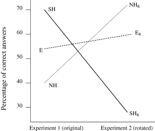
Figure 6 reveals that 180° rotation did not affect the results at the equator (E) nearly as much as in the NH and SH images. This could mean more ambiguity ‘in the middle’; however, at this point we decided not to include the three images that were taken from the equator region (located at 0° latitude) in further analysis, and to focus on the NH and SH images. This decision was motivated by the fact that the stimuli sample from the equator region was too small (n = 3). For the NH and SH images, and for the rotated NH and SH images (NH_R and SH_R), Figure 6 clearly shows what we expected to see: participants make more mistakes in identifying the landforms with the NH set before rotation, and fewer mistakes after; this is reversed for the SH set.

Main hypothesis testing

The interaction plot (Figure 6) indicates that the variables in the experiment led to a change in performance; however, this does not demonstrate if the results are statistically significant or not. Therefore, at this stage, we address two main questions based on inferential statistics: (1) whether the majority of the participants experience terrain reversal illusion in the NH sample and do not experience the illusion in the SH sample and (2) whether rotating the images 180° reverses the results for the majority of the tested population and the majority of the images. However, before we conducted inferential statistics, to understand the ‘spread’ of the correct/incorrect answers per stimuli group, we obtained a (descriptive) box-and-whisker plot of the raw data (Figure 7).

Figure 7. Box-and-whisker plots of raw data showing percentage of correct answers per stimuli group. The solid line inside the box is the median. Boxes cover the interquartile range, whiskers extend 1.5 interquartile range from the boxes, and outliers outside this range are indicated with points.

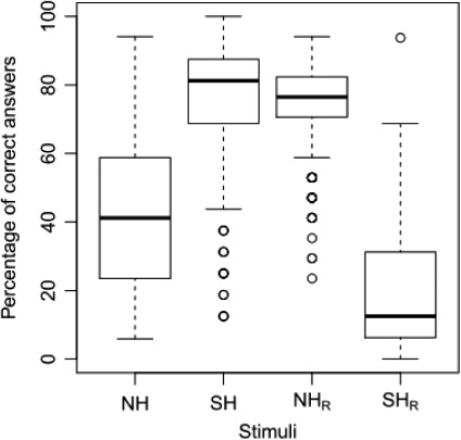
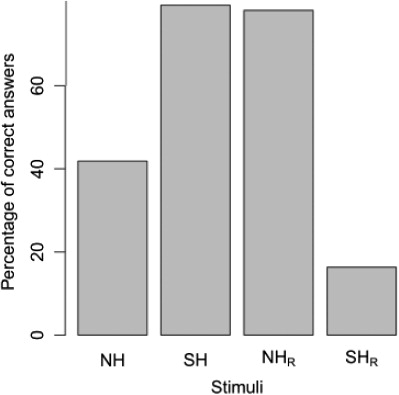
When participants viewed the original NH images, only 40.3% of the landforms are correctly identified (60.7% were not). The percentage of correct answers rose to 75.5% in the original SH sample (only 24.5% incorrect answers). In Experiment 2, where stimuli were rotated 180°, the results were practically reversed: 72% of participants correctly identify the terrain features in the rotated NH images (NH_R) and only 28% in the rotated SH images (SH_R) (Figure 7).

To test the reliability of the differences observed in Figure 7, we analyzed the data by means of inferential statistics using the generalized linear mixed-effect model as implemented by Bates et al. 2013 in R (R Core Team 2014). We fit a linear model with binomial errors (logistic regression) where we specify ‘image’ and ‘participant’ as ‘random effects’. In the current analysis, we do not focus on the difficulty of a particular image or individual differences, but the difficulty of images grouped according to the NH and SH, NH_R and SH_R. The estimates in Table 2 confirm that the illusion is more prevalent in the images from the NH in a statistically significant manner. That is, people are less likely to respond correctly to the questions when presented with the images from the NH sample while the images from the SH sample are more likely to be interpreted correctly. We can also confirm that the rotation reverses these predictions in a statistically significant manner.

Table 2. Estimates of fixed-effect parameters of binary generalized linear mixed-effect models on questionnaire data.

	Estimate	Standard error	z value	p value
Intercept (NH)	−0.33	0.17	−1.90	0.057
SH	1.68	0.24	6.87	6.61 × 10^−12
NHR	1.60	0.07	21.90	<2 × 10^−16
SHR	−4.58	0.08	−55.82	<2 × 10^−16

Although one can reach these conclusions from Table 2 and can see the certainty of the estimates, the outcome of the binomial regression is somewhat difficult to map directly to the problem we have at hand. To aid the interpretation of the model's results, we present the model's predictions (for each case we are interested in) in Figure 8, confirming and explicitly communicating the same message as Table 2.

Figure 8. Estimated correct answer rates based on inferential statistics for images from NH and SH before and after the rotation (NH_R and SH_R). The values were obtained from the generalized linear model estimates presented in Table 2 and transformed back to the response scores (expected success rate).

Exploratory analysis of group differences

As mentioned earlier, the experimental design does not control for group differences, i.e. we recruited participants without counterbalancing for different characteristics. However, after testing for the main effects, we conducted exploratory analyses on the possible group differences as we have the background data (Table 1), because such analyses may lead to new hypotheses. Utilizing ordinary least squares regression, the question differences were collapsed into a single rate of success per participant. Since the number of participants was fairly high, the binomial distribution is well approximated by a normal distribution, and the model diagnostics also confirm this. We first present a model where success rate was predicted by all individual characteristics asked prior to the completion of the questionnaires; namely age, gender, education, specialization (geopro), experience in using 3D graphics (threeD), confidence in photo interpretation (photoconf), and whether there were known problems with their color vision (colorvision). The model estimates are presented in Table 3.

Table 3. Estimates of full model

	Estimate	Standard error	t value	Pr(>∣t∣)
(Intercept)	0.2283	0.1457	1.57	0.1173
Age	0.0001	0.0001	0.60	0.5499
Gender:male	0.0416	0.0209	1.99	0.0471
Education	0.0036	0.0264	0.14	0.8902
Geopro	0.0315	0.0156	2.02	0.0437
ThreeD	0.0099	0.0154	0.64	0.5206
Photoconf	0.0032	0.0261	0.12	0.9010
Colorvision	0.0426	0.0497	0.86	0.3908

Note: Except gender, all other variables take numeric values. R² = 0.02, Adj-R² = 0.01, F(7,940) = 2.847, p value = 0.006.

In this analysis, we find significant effects due to gender (men seem to make fewer mistakes at first sight) and profession (geoprofessionals seem to make fewer mistakes at first sight). However, it is critical to note that the percentage of the variation explained by this model is only about 2%, indicating that essentially none of the individual characteristics that we recorded had a substantial effect. According to this model, the effect sizes for the two significant effects due to gender and profession are rather low: we expect male participants to answer 4% more correctly, and for each step of the five-level variable geoprofessional, we expect a 3% increase in correct responses. Furthermore, since our experimental design is not counterbalanced (in the sample, we have more males who are geoprofessionals), drawing conclusions from this analysis is not viable. To investigate the two strongest predictors in some more detail, we ran another analysis where we used only these two predictors and their interaction. Table 4 presents the estimates of an ordinary least squares regression model that predicts rate of success from gender and geoprofessional variables and their interactions.

Table 4. Estimates of the model with gender and geoprofession as predictors.

	Estimate	Standard error	t value	Pr(>∣t∣)
(Intercept)	0.3815	0.0727	5.24	<0.0001
Gender:male	−0.0214	0.0932	−0.23	0.8181
Geopro	0.0290	0.0172	1.69	0.0918
Gender:male × Geopro	0.0149	0.0217	0.69	0.4927

Note: R² = 0.02, Adj-R² = 0.02, F(3,944) = 6.305, p value = 0.0003.

The variation explained does not decrease and this indicates that most of the (rather small) variation explained by individual differences is indeed due to these two variables. Furthermore, the smaller model reveals the fact that the significant differences due to gender found in the full model are probably due to sampling bias (more males in the ‘geopro’ sample). Although the estimates now are even less certain, the significance of the estimate due to gender is reversed, further indicating that the reason for the higher rate of success by male participants is likely due to the fact that more of the male participants work in geo-related professions in comparison to the female participants in our study. The fact that the ‘geopro’ group seem to make fewer mistakes might be because they interpret land-use/land-cover cues more carefully, or they take the task seriously and search for the location (the location names were known to the participants) by other means.

Discussion

In summary, our findings give three main results: First, our qualitative image surveys suggest that the illusion appears to be indeed more common when viewing the NH images. Further systematic and rigorous studies are necessary to confirm this and assess exactly where (at which latitudes) the illusion occurs most commonly; nonetheless, our findings allow us to hypothesize that the terrain reversal is more commonly experienced in the NH. Several other researchers suggested this in the literature. However, previous studies were mainly without empirical evidence, either based on direction of illumination theory or qualitative reasoning (e.g. Saraf et al. 1996; Berbané-Poveda, Manso-Callejo, and Ballari 2005). Our findings show that the SH is not entirely free from the illusion; however, there are considerably fewer instances than in the NH according to our observations. Again, further studies are needed to document the true extent of the issue in the SH. Second, the online user experiment empirically confirms that the majority of people will experience this illusion when presented with images sampled form the NH and 180°-rotated SH images (SH_R). Third, 180° rotation is a ‘strong fix’ for this illusion where the illusion is present (NH → NH_R), but where the illusion is not present in the original imagery, it introduces a strong terrain reversal effect (SH → SH_R), which is undesirable (Figure 7).

The terrain reversal effect is most relevant when the terrain is rugged, however, even with rugged terrains; we observe that when one individual experiences terrain reversal with one image, another individual may not. With this study, we were able to empirically confirm that the majority of people experience the illusion when viewing the same images. One should also note that we did not control for the scene content, that is, we did not account for dominant landforms, their orientation, and seasonality of the images in this study. Therefore, the land cover (snow, vegetation, rivers, and similar) may have given ‘logical’ top-down (cognitive, instead of perceptual) cues for some people to reconsider their bottom-up perception. In other words, the top-down cognitive signal might be suppressing the bottom-up perceptual signal. For example, participants may perceive a valley, but if there is snow on the valley floor and just next to it a green belt, they may think ‘this is probably a trick question’, and respond ‘ridge’. Similarly, if there is a river that appears to follow a ridge, this allows for interpretation that this feature is most likely a valley. We believe it is especially likely with geoprofessionals to double check against their perception, because they are trained to interpret the terrain features and could find resources to confirm. Yet another factor might be that some participants are possibly familiar with the region, thus may know the ‘correct answer’ already. However, all these factors clearly do not detract from our results. Such cues would help people make fewer mistakes, thus we might currently have ‘false success’ in our results. If we had controlled for these factors, we might have found an even stronger difference, and therefore, our findings would be further confirmed, not challenged. A follow-up controlled laboratory study with eye tracking is in progress which will allow us to account for these factors, as well as possible explanations about the behavior of those participants who seemingly do not experience this illusion.

Exploration of group differences yielded interesting but inconclusive results in this study. What we can say at the moment is that people experience this illusion, regardless of their background. This might change in a study that is optimized to measure group differences. At this point, we observe a weak positive effect based on expertise; which suggests that the experts may be using their previous knowledge about landforms and land cover to override the perceptual signals. However, properly establishing the impact of expertise on experiencing the terrain reversal effect remains to be explored in a follow-up study in a controlled laboratory environment.

The main message in this paper is that the majority of participants failed to identify the landform correctly in the original NH sample and in the rotated SH_R imagery, regardless of their background. This also happened despite several auxiliary cues in some of the imagery such as rivers, roads, and lakes in odd positions or unrealistic distribution of snow/vegetation cover on mountains/valleys. These findings indicate that the effect is very strong and very commonly experienced. We need further studies to establish the exact locations (and recording time) of the satellite images for the NH imagery and seek solutions, and we need to find out how to deal with interactive globes where people may rotate the display and ‘create’ this illusion unintentionally.

Conclusions and outlook

The study presented in this paper directly contributes to geovisual analytics and digital earth research as it establishes the prevalence of a perceptual phenomenon, i.e. helps in pinning down the importance of the terrain reversal effect for geovisualization displays (specifically in naturally lit satellite imagery). The results motivate and validate efforts to solve the issue, as well as helping to raise awareness among the map providers and map users who work with visual analysis and photo interpretation. Now with empirical evidence, we can say that this phenomenon should not be neglected, especially if/when the photo interpretation is of critical importance.

At this point, the question of ‘how to “fix” the problem?’ arises. Rotating the display is not a good solution; first of all, as this study confirms, it can introduce terrain reversal effect where it was not present, but also we lose our conventional North reference by rotating the display (and ‘mental rotation’ is a hard task). Inverting the colors (‘negative’ of the image) is clearly not a usable solution because we rely on color information to perceive classes and patterns. Several solutions based on selective modification of color information and use of hypsographic coloring have been proposed in literature regarding this problem (see Wu, Li, and Gao 2013; Bernabé-Poveda, Sánchez-Ortega, and Çöltekin 2011; Saraf et al. 2007; Kettunen and Sarjakoski 2009); however, none of them are user tested at this point. Another follow-up study will be on user testing the proposed solutions and assessing them for their ease of implementation.

Acknowledgements

Authors wish to express their sincere gratitude to Dr Çağrı Çöltekin for statistics advice, Ms Laura Blumenthal for language revisions, Mr Iván Moya Honduvilla for helping with data collection, Ms Juliette Marx for her valuable help as a participant in qualitative reviews of landforms, and the anonymous reviewers for their valuable feedback on various important issues of clarification and consistency.

References

- Amit, R., E. Zilberman, N. Porat, and Y. Enzel. 1999. “Relief Inversion in the Avrona Playa as Evidence of Large-Magnitude Historical Earthquakes, Southern Arava Valley, Dead Sea Rift.” Quaternary Research 52: 76–91. doi:10.1006/qres.1999.2050.
- Arnheim, R. 1976. “The Perception of Maps.” Cartography and Geographic Information Science 3: 5–10. doi:10.1559/152304076784080276.
- Bates, D., M. Maechler, B. Bolker, and S. Walker. 2013. lme4: Linear Mixed-Effects Models Using Eigen and S4. R package version 1.0-4. http://cran.r-project.org/web/packages/lme4/index.html.
- Bernabé-Poveda, M. A., M. A. Manso-Callejo, and D. Ballari. 2005. “Correction of Relief Inversion in Imaes Served by a Web Map Server.” In Proceedings of the International Cartographic Conference, ICC 2005, A Caruna, Spain.
- Bernabé-Poveda, M. A., I. Sánchez-Ortega, and A. Çöltekin. 2011. “Techniques for Highlighting Relief on Orthoimagery.” Procedia – Social and Behavioral Sciences 21: 346–352. doi:10.1016/j.sbspro.2011.07.028.
- Boer, A., A. Çöltekin, and K. C. Clarke. 2013. “Evaluating Web-based Geovisualizations Online: A Case Study with Abstraction-Realism Spectrum in Focus.” In Proceedings of the International Cartographic Conference, ICC 2013, Dresden, Germany.
- Cleveland, W. S. 1983. “A Color-Caused Optical Illusion on a Statistical Graph.” The American Statistician 37: 101–105.
- Çöltekin, A., and T. Reichenbacher. 2011. “High Quality Geographic Services and Bandwidth Limitations.” Future Internet 3: 379–396. doi:10.3390/fi3040379.
- Gilmartin, P. P. 1981. “The Interface of Cognitive and Psychophysical Research in Cartography.” Cartographica: The International Journal for Geographic Information and Geovisualization 18: 9–20. doi:10.3138/BN50-8GU9-226R-62K1.
- Howard, I. P. 2002. “Shading and Shadows.” In Seeing in Depth, Vol 1. Basic Mechanisms, edited by Ian P. Howard, 391–399. Toronto: I.Porteous.
- Imhof, E. 1967. “Shading and Shadows.” In Cartographic Relief Representation, edited by H. J. Steward, 159–212. Redlands, CA: ESRI Press.
- Jenny, B., and T. Patterson. 2007. “Introducing Plan Oblique Relief.” Cartographic Perspectives Spring, 21–40.
- Kettunen, P., and T. Sarjakoski. 2009. “Cartographic Portrayal of Terrain in Oblique Parallel Projection.” In Proceedings of the International Cartographic Conference, Santiago, Chile, November 15–21.
- Khang, B.-G., J. J. Koenderink, and A. M. L. Kappers. 2006. “Perception of Illumination Direction in Images of 3-D Convex Objects: Influence of Surface Materials and Light Fields.” Perception 35: 625–645. doi:10.1068/p5485.
- Kleffner, D., and V. S. Ramachandran. 1992. “On the Perception of Shape from Shading.” Perception & Psychophysics 52: 18–36. doi:10.3758/BF03206757.
- Liu, B., and J. T. Todd. 2004. “Perceptual Biases in the Interpretation of 3D Shape from Shading.” Vision Research 44: 2135–2145. doi:10.1016/j.visres.2004.03.024.
- Pain, C., J. Clarke, and M. Thomas. 2007. “Inversion of Relief as a Geomorphic Process on Mars and Its Relevance to Landing Site Selection.” In Australian Mars Exploration Conference (AMEC), 4–10, Perth, Australia, July 13–15.
- Pain, C. F., and J. D. A. Clarke. 2009. “Relief Inversion: Australian Analogs of a Common Feature of Martian Landscape Evolution.” In Lunar and Planetary Science Conference, 5–6, The Woodlands, TX, March 23–27.
- Pain, C. F., and C. D. Oilier. 1995. “Inversion of Relief — a Component of Landscape Evolution.” Geomorphology 12 (2): 151–165. doi:10.1016/0169-555X(94)00084-5.
- Patterson, T. 2013. Illumination. ShadedReliefArchive.com—A Digital Repository for Cartographic Relief Art. Accessed October 14. http://www.shadedrelief.com/retro/discussion.html
- Pinna, B., and G. Mariotti. 2006. “Old Maps and the Watercolor Illusion: Cartography, Vision Science and Figure-Ground Segregation Principles.” In Systemics of Emergence: Research and Development, edited by G. Minati, E. Pessa, and M. Abram, 261–278. New York, NY: Springer US.
- Prados, E., and O. Faugeras. 2006. “Shape from Shading.” In Handbook of Mathematical Models in Computer Vision, edited by N. Paragios, Y. Chen, and O. Faugeras, 375–388. New York, NY: Springer Science+Business Media.
- R Core Team. 2014. R: A Language and Environment for Statistical Computing. R Foundation for Statistical Computing. http://www.r-project.org/
- Rudnicki, W. 2005. “Perspective Views and Panoramas in Presentation of Relief Forms in Poland.” In Proceedings of the International Cartographic Conference (ICC), A Coruna, Spain, July 9–16.
- Saraf, A. K., J. D. Das, B. Agarwal, and R. M. Sundaram. 1996. “False Topography Perception Phenomena and Its Correction.” International Journal of Remote Sensing 17: 3725–3733. doi:10.1080/01431169608949180.
- Saraf, A. K., S. T. Sinha, P. Ghosh, and S. Choudhury. 2007. “A New Technique to Remove False Topographic Perception Phenomenon and Its Impacts in Image Interpretation.” International Journal of Remote Sensing 28: 811–821. doi:10.1080/01431160701269796.
- Saraf, A. K., M. Zia, J. Das, K. Sharma, and V. Rawat. 2011. “False Topographic Perception Phenomena Observed with the Satellite Images of Moon's Surface.” International Journal of Remote Sensing 32: 9869–9877. doi:10.1080/01431161.2010.550950.
- Toutin, T. 1998. “Depth Perception with Remote Sensing Data.” In Proceedings of the 17th EARScL Symposium on Future Trends in Remote Sensing, edited by Gudmandsen, 401–409. Lyngby, Demark: A.A. Balkema/Rotterdam/Brookfield.
- Wood, M. 1968. “Visual Perception and Map Design.” The Cartographic Journal 5: 54–64. doi:10.1179/caj.1968.5.1.54.
- Wu, B., H. Li, and Y. Gao. 2013. “Investigation and Remediation of False Topographic Perception Phenomena Observed on Chang'E-1 Lunar Imagery.” Planetary and Space Science 75: 158–166. doi:10.1016/j.pss.2012.10.018.
- Zhou, A., X. Zhang, and L. Gao. 2006. “DEM Terrain Reversal.” Geography and Geo-Information Science 22: 42–44.