Rapid, high-resolution detection of environmental change over continental scales from satellite data – the Earth Observation Data Cube

ABSTRACT

The effort and cost required to convert satellite Earth Observation (EO) data into meaningful geophysical variables has prevented the systematic analysis of all available observations. To overcome these problems, we utilise an integrated High Performance Computing and Data environment to rapidly process, restructure and analyse the Australian Landsat data archive. In this approach, the EO data are assigned to a common grid framework that spans the full geospatial and temporal extent of the observations – the EO Data Cube. This approach is pixel-based and incorporates geometric and spectral calibration and quality assurance of each Earth surface reflectance measurement. We demonstrate the utility of the approach with rapid time-series mapping of surface water across the entire Australian continent using 27 years of continuous, 25 m resolution observations. Our preliminary analysis of the Landsat archive shows how the EO Data Cube can effectively liberate high-resolution EO data from their complex sensor-specific data structures and revolutionise our ability to measure environmental change.

KEYWORDS:

• Earth Observation Data Cube
• HPD
• HPC
• surface water
• Landsat
• Australia

1. Introduction

Satellite Earth Observation (EO) data have long been recognised for the unique, globally consistent information that they contain. However, the wealth of information available in EO data, especially records with a long time-series, wide extent and high (<100 m) spatial resolution (e.g. Landsat, SPOT, ASTER archives) is yet to be fully exploited. In addition to their size, these EO data represent a particular type of highly structured data that present challenges for their integration, analysis and application (Wulder and Coops 2014). This is compounded by variability in the observing conditions (e.g. atmospheric conditions, obscuration by clouds and changes in viewing geometry) and differences between individual sensors used to collect observations from multiple spacecraft (e.g. different spatial, spectral and radiometric resolutions).

Most applications of satellite data involve transformation of the signals collected by the sensor (‘Level 0’ raw data) to geophysical measurements of physical properties of the Earth's surface (‘Level 3’ gridded, calibrated measurements). Other applications involve multistage processes of generating and refining geophysical models through iterative comparison and regression of simulated data with observed Level 1, 2 and 3 measurements (Teixeira et al. 2014). These processes are time-consuming and therefore costly, and greatly increase the volume of data to be managed. Consequently, despite the potential value of these data, few continental-scale datasets have been developed at the spatial resolution of Landsat observations (Lehmann et al. 2013) and there are no continental-scale time-series that utilise all the available observations over decadal time-spans.

Here we provide an initial overview of our innovative approach to the processing, restructuring and analysis of EO data in an integrated High Performance Computing – High Performance Data (HPC-HPD) environment. To demonstrate the speed and utility of this approach we present the preliminary results of the analysis of surface water across the entire Australian continent (7.6 million km²) using the full 27 years of Landsat Thematic Mapper observations. Importantly, algorithms that identify the dynamics of other land cover themes can be applied to the same EO data. Our approach significantly progresses the concept of Digital Earth by enabling more effective and efficient analysis of EO data over their full spatial and temporal dimensions.

2. Data

The Australian Landsat archive, acquired continuously from 1987 to 2014 (25 m resolution; observation frequency: 8–16 days) includes data from the Landsat 5 Thematic Mapper (TM) and Landsat 7 Enhanced Thematic Mapper Plus (ETM+) sensors (archive details available at http://dx.doi.org/10.4225/25/5487CC0D4F40B). The data were moved from tape archives at Geoscience Australia to the National Computing Infrastructure (NCI) Facility at the Australian National University.

3. Method

To very rapidly convert the Landsat data archive into useful geophysical variables, processing and analysis were performed on the integrated HPC-HPD resources at the NCI. The data were placed on NCI's site-wide persistent high bandwidth Lustre file system, connected with I/O speeds of 56 GBytes/sec. The file system is mounted on a High Performance Cloud, using OpenStack software with 3000 Intel SandyBridge cores. This provides a hybrid of HPC and data-intensive computation infrastructure (Evans et al. 2015) that allows users and data services to interactively invoke different forms of computation, in situ, over large-volume data collections.

3.1. Data processing

The following steps were undertaken to calibrate and restructure the archive at the NCI:

Step 1: The conversion of data from satellite telemetry to geometrically corrected images utilised the Level 1 Product Generation System code developed by the United States Geological Survey (Loveland and Dwyer 2012).

Step 2: An automated spectral calibration and quality assessment of the observations included correction for atmospheric interference and for illumination and viewing angles (Li et al. 2012). This produced a standardised measure of surface reflectance, with data quality flagged for each pixel (e.g. presence of cloud) (Sixsmith, Oliver, and Lymburner, 2013).

Step 3: Data within each satellite image were spatially segmented into 1° × 1° tiles, the tiles forming a grid that covers the Australian continent (Figure 1). This restructuring is based on an equal-angle global grid tessellation that enables efficient use of the parallel capabilities of HPC.

Figure 1. Landsat scenes compared with the 1° × 1° data tiles employed in the EO Data Cube. The Landsat scenes capture Brooks Island in Lake Eyre in 2009. The spatial footprint of Landsat scenes changes over time, while the data tiles maintain a constant footprint.

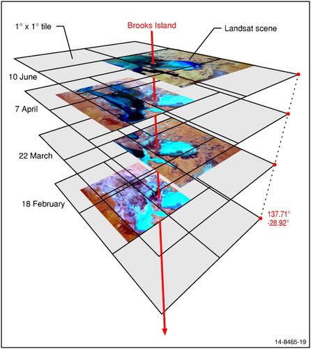
The reformatted data were indexed in a PostgreSQL relational database, with the 1,744,884 1° × 1° tiles stored on the Lustre file system (details of the output data are available at http://dx.doi.org/10.4225/25/5487CC0D4F40B). The output represents a space-time EO Data Cube in which the time-series of calibrated surface reflectance observations (pixels) of the same location are captured in a series of data tiles that have an identical geospatial footprint (Figure 1).

3.2. Surface water analysis

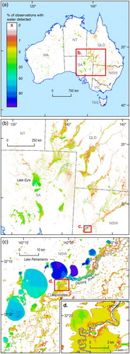
This analysis was undertaken to demonstrate the application of the EO Data Cube. To detect surface water, a regression tree classification analysis was undertaken on the Landsat surface reflectance observations (Step 3 output). Data were rapidly distributed across thousands of compute nodes for parallel computation, underpinned by the high-performance Lustre file system. Training data for the classification algorithm were selected from a total of 59 Landsat scenes and a separate set of 34 scenes were used to test the accuracy of the algorithm. The resulting decision tree used a combination of four Thematic Mapper bands and three Normalized Difference Indices to classify observations as ‘water’ or ‘non-water’, with an overall accuracy of 97%. Errors occurred where there was both water and vegetation within a pixel and due to low sunlight. The classification was summarised across the temporal range for every pixel as the ratio of water to non-water observations (Figure 2; details of the methods are available at http://dx.doi.org/10.4225/25/5487D7B920F51).

Figure 2. Landsat observations of surface water across Australia, expressed as a percentage of the 27 years of observations for every 25 m pixel. (a) The extensive arid areas are clearly identified (colour key applies to all figures). (b) The highly ephemeral character of rivers and lakes and diffuse flow patterns of rivers are evident. (c) The Menindee Lakes water storage contrasts with the surrounding low-relief landscape that experiences highly infrequent but extensive occurrence of surface water. (d) An example of the fine-scale resolution of observations for the Darling River floodplain.

4. Results

Over 10¹² individual observations were processed to complete the initial surface water analysis (Figure 2), drawn from over 300,000 Landsat scenes, yet the processing was completed in less than 6 hours. Fundamental to this computational efficiency is the spatial segmentation of the calibrated Landsat data into 1° × 1° tiles, a structure independent of the original scene-based format (Figure 1).

The presence and frequency of occurrence of surface water is shown across spatial scales ranging from a few tens of metres to the entire continent (Figure 2(a)–(d)). For many regions in Australia the spatial and temporal extents of significant stream flows and floods have never been mapped in this robust, detailed way (Figure 2(b), (c)). Clearly visible is the infrequent detection of water, reflecting the highly ephemeral nature of river flows across most of the Australian continent.

5. Discussion

In our analysis of the Landsat archive, over 600 possible observations were available per pixel, and up to 1200 observations in areas where adjacent satellite paths overlap. In contrast, a more traditional scene-based sampling approach (e.g. Masek et al. 2008) would only use about 60 observations over 27 years, limiting the ability to detect change.

The Landsat EO Data Cube comprises geometrically and spectrally calibrated surface reflectance observations related to the WGS84 datum, providing a robust, authoritative dataset for the Australian continent (cf., Google Earth Engine Landsat archive). Importantly, the Landsat 1° × 1° data tiles have a fixed and consistent footprint and are linked in a relational database, providing a highly efficient structure for EO data analysis in an integrated HPC-HPD environment, key elements of the EO Data Cube. This approach could similarly be applied in other continents and to other types of EO data to more effectively and rapidly analyse the dynamics of important land cover themes (e.g. forest cover and land-use change).

6. Summary

To enable the rapid analysis of high-resolution EO data, we have developed a HPD structure, set within a high performance, data-intensive computing system. Data are assigned to a common grid framework that spans the full geospatial and temporal extent of the observations. This approach is pixel-based and incorporates the calibration and quality assurance of each Earth surface reflectance measurement, transforming EO Big Data into data that can be accessed and rapidly analysed in integrated HPC-HPD environments.

Acknowledgments

Thanks to Bryan Lawrence (University of Reading), Clinton Foster and David Lescinsky (GA) and two anonymous reviewers for useful comments, and Chris Evenden (GA) for drafting the figures. This research was funded by the Commonwealth of Australia and the ANU's NCI Facility. GA staff publish with permission of the Chief Executive Officer, Geoscience Australia.

Disclosure statement

No potential conflict of interest was reported by the authors.

References

- Evans, B., L. Wyborn, T. Pugh, C. Allen, J. Antony, K. Gohar, D. Porter, et al., 2015. “The NCI High Performance Computing (HPC) and High Performance Data (HPD) Platform to Support the Analysis of Petascale Environmental Data Collections.” In Environmental Software Systems: Infrastructures, Services and Applications, edited by Ralf Denzer, Robert M. Argent, Gerald Schimak, and Jiří Hřebíček, 569–577. Springer. http://link.springer.com/chapter/10.1007%2F978-3-319-15994-2_58.
- Lehmann, E. A., J. F. Wallace, P. A. Caccetta, S. L. Furby, and K. Zdunic. 2013. “Forest Cover Trends from Time Series Landsat Data for the Australian Continent.” International Journal of Applied Earth Observation and Geoinformation 21: 453–462. doi: 10.1016/j.jag.2012.06.005
- Li, F., D. L. Jupp, M. Thankappan, L. Lymburner, N. Mueller, and A. Lewis. 2012. “A Physics-Based Atmospheric and BRDF Correction for Landsat Data over Mountainous Terrain.” Remote Sensing of the Environment 124: 756–770. doi: 10.1016/j.rse.2012.06.018
- Loveland, T. R., and J. L. Dwyer. 2012. “Landsat: Building a Strong Future.” Remote Sensing of the Environment 122: 22–29. doi: 10.1016/j.rse.2011.09.022
- Masek, J. G., C. Huang, W. B. Cohen, J. Kutler, F. G. Hall, R. Wolfe, and P. Nelson. 2008. “North American Forest Disturbance Mapped from a Decadal Landsat Record: Methodology and Initial Results.” Remote Sensing of the Environment 112: 2914–2926. doi: 10.1016/j.rse.2008.02.010
- Sixsmith, J., S. Oliver, and S. Lymburner. 2013. “A Hybrid Approach to Automated Landsat Pixel Quality.” Geoscience and Remote Sensing Symposium (IGARSS), 2013 IEEE International, Melbourne, VIC, July 21–26, 4146–4149. http://ieeexplore.ieee.org/xpl/login.jsp?tp=&arnumber=6723746&url=http%3A%2F%2Fieeexplore.ieee.org%2Fxpls%2Fabs_all.jsp%3Farnumber%3D6723746.
- Teixeira, J., D. Waliser, R. Ferraro, P. Gleckler, T. Lee, and G. Potter. 2014. “Satellite Observations for CMIP5: The Genesis of Obs4MIPs.” Bulletin American Meteorological Society 95: 1329–1334. doi: 10.1175/BAMS-D-12-00204.1
- Wulder, M. A., and N. Coops. 2014. “Satellites: Make Earth observations open access.” Nature 513: 30–31. doi: 10.1038/513030a