Forward a spatio-temporal trend surface for long-term ground-measured albedo upscaling over heterogeneous land surface

ABSTRACT

Upscaling ground albedo is challenged by the serious discrepancy between the heterogeneity of land surfaces and the small number of ground-based measurements. Conventional ground-based measurements cannot provide sufficient information on the characteristics of surface albedo at the scale of coarse pixels over heterogeneous land surfaces. One method of overcoming this problem is to introduce high-resolution albedo imagery as ancillary information for upscaling. However, due to the low frequency of updating of high-resolution albedo maps, upscaling time series of ground-based albedo measurements is difficult. This paper proposes a method that is based on the idea of conceptual universal scaling methodology for establishing a spatiotemporal trend surface using very few high-resolution images and time series of ground-based measurements for spatial-temporal upscaling of albedo. The construction of the spatiotemporal trend surface incorporates the spatial information provided by auxiliary remote sensing images and the temporal information provided by long time series of ground observations. This approach was illustrated by upscaling ground-based fine-scale albedo measurements to a coarse scale over the core study area in HiWATER. The results indicate that this method can characterize the spatiotemporal variations in surface albedo well, and the overall correlation coefficient was 0.702 during the study period.

KEYWORDS:

• Trend surface
• upscaling
• spatiotemporal
• heterogeneous
• albedo

1. Introduction

Surface albedo determines the amount of solar radiation absorbed by the land surface (Dickinson 1995; Liang 2003; Souza et al. 2006; Liu et al. 2009; Wen et al. 2009). It is a key factor in determining the surface energy budget and is often used in applications such as climate, hydrological and biogeochemical models. Satellite remote sensing products provide a unique way to acquire surface albedo globally (Liang 2001, 2005). However, these products suffer from lots of uncertainties, due to the inherent complexity of the relevant physical processes and their parameterizations. In addition, these uncertainties continuously affect quantitative remote sensing applications. In general, the accuracy and uncertainty of satellite albedo products should be assessed using reliable reference or ground truth data. This process is termed validation.

One of the important steps in validation is performing spatiotemporal matching between the satellite albedo products and ground-based albedo measurements. The literature (Jin et al. 2003; Wang et al. 2004; Stroeve et al. 2005; Chen et al. 2008; Wang et al. 2010; Stroeve et al. 2013) shows that the mismatches in spatial scale between satellite-based albedo and ground-based albedo over homogeneous land surfaces can be ignored when the ground-based albedo is considered to be spatially representative. However, it presents important challenges over heterogeneous land surfaces, because the spatial scale of ground-based albedo is so small compared with the spatial resolution of coarse-scale satellite pixels that it cannot represent the true value at the coarse-pixel scale. Thus, upscaling fine-scale ground-based albedo measurements to the coarse-pixel scale obtained from satellite has become an important scientific issue in the process of validation.

The main challenge involved in upscaling is that the ground-based measurements cannot provide sufficient heterogeneous information extending to the pixel scale over heterogeneous land surfaces (Román, Gatebe, and Shuai 2013). An alternative method is known as multi-scale validation (Liang et al. 2002; Peng et al. 2014; Mira et al. 2015). In this case, an albedo map with high spatial resolution provides the spatial distribution characteristics of the surface albedo and thus captures its heterogeneity. It is used as a bridge for upscaling to reduce the scale discrepancy between fine-scale ground-based and coarse-scale satellite-based observations. In this method, ground-based albedo is used to calibrate high-resolution albedo maps. The calibrated high-resolution albedo maps are aggregated (i.e. averaged) to provide the relative truth at the coarse-pixel scale. However, in this process, the errors from both the high-resolution albedo maps and the calibration coefficients will deviate from the ‘truth’ at coarse-pixel scale and introduce uncertainty into the validation results. Another method is regression kriging (RK) (Hengl, Heuvelink, and Rossiter 2007), which divides the land surface parameter into the trend surface and residuals. Crow et al. (2012), Kang, Jin, and Li (2015) and Ge et al. (2015) have applied RK technique to upscale soil moisture and sensible heat fluxes over heterogeneous land surfaces and confirmed that the residuals are more realistic to satisfy the assumption of stationarity of kriging. The albedo trend surface is established based on high-resolution albedo imagery, which is equivalent to the calibration process. On the other hand, the residuals represent the bias between the ground-based albedo and the trend surface, which is the counterpart of the errors remaining in the multi-scale validation method. Thus, the RK technique can compensate for the errors remaining in the multi-scale validation (Wu et al. 2016).

However, upscaling processes of multi-scale validation and RK technique are heavily dependent on the quality of high-resolution satellite albedo. And its low update frequency will prevent coarse-scale albedo product validation continuously over long time periods. The temporal-scale mismatch between the coarse-pixel albedo products and the high-resolution albedo maps can result in uncertainty in the validation, due to the inability to characterize the dynamic change of land surfaces (Camacho et al. 2013). Thus, neither the multi-scale validation nor the RK technique can satisfy the requirement for an overall validation for albedo remote sensing products, which should involve not only a complete spatial validation including different typical land covers, but also a complete temporal validation over a typical cycle period.

Wang, Xie, and Li (2014) proposed the concept of geographic trend surfaces and established a universal scaling methodology. In this conceptual methodological framework, the geographic trend surface is constructed first. It is then adjusted within spatial and temporal frames fusing temporally varying records. Finally, the land surface parameters can be derived at the desired scales. This methodology lays the foundation for addressing problems related to a lack of information or key information reservation in scaling. Nevertheless, this theory has not been put into practice.

Stemming from the methodology of geographic trend surface, this paper aims to develop a method for identifying spatiotemporal trend surface that supports upscaling ground-based albedo spatially and temporally to derive ground albedo truth at coarse-pixel scales for validation of coarse-scale satellite albedo products over heterogeneous land surfaces. The spatiotemporal trend surface, which is independent of the frequency and absolute value of high-resolution albedo maps, is proposed to characterize the spatiotemporal heterogeneous component of surface albedo. Further, its performance is assessed by comparing it with temporally continuous ground-based measurements. This method is illustrated using one Compact Airborne Spectrographic Imager (CASI) image and the wireless sensor network (WSN)-based ground data over the core study area of HiWATER (Li et al. 2013). Section 2 of the paper describes the study area and the data. Section 3 explains the method used to construct the spatiotemporal trend surface. Section 4 shows the resulting trend surface, the upscaling results and a preliminary validation of multiple types of coarse-scale albedo products. A brief conclusion is provided at the end.

2. Study area and data

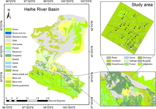
The study area is located in the middle reaches of the Heihe River Basin, which is a typical inland river basin that has served as an experimental region for integrated watershed studies, as well as remote sensing research (Li et al. 2013). A 5.5*5.5 km area (Figure 1) covering the region bounded by 38°50′–38°54′ N and 100°19′–100°24′ E was selected as the albedo product validation region. Many land cover types are present within this region (Figure 1), including cornfields, wheat fields, vegetable fields and orchards. Additionally, buildings, roads, and greenhouse and irrigation channels are also present. The WSN observations extend from 10 June 2012 to 16 September 2012, which correspond to day of year (DOY) 162 to DOY 260. These observations were made at 17 nodes that were distributed according to the distribution of, for example, crop structure, windbreaks, residential areas, soil moisture and irrigation status (Xu et al. 2013; Liu et al. 2016). Of these nodes, node 1 is in a vegetable field, node 4 is within a built-up area, node 17 is in an orchard, and the others are in corn fields.

Figure 1. Map of the study area and the distribution of the WSN nodes (projection: WGS_1984_UTM_Zone_47N)

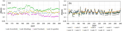
Each node was instrumented with Kipp and Zonen radiometers measured the total downward and upward shortwave radiation. Details of the performance of the radiometers and inter-comparisons of radiometers can be found in (Xu et al. 2013). Both radiometers were mounted 3 m above the canopy and have a footprint of approximately 26 m in diameter (Sailor, Resh, and Segura 2006). These radiometers take radiation measurements at 10-min intervals. As the satellite products provide local solar noon albedo values, the average downward and upward radiation values around local solar noon under clear-sky conditions were extracted to generate ground-based albedo on a daily basis. The surface albedo over the study area is highly spatially variable both intra-type and inter-types. Different surface types show albedo values with differences of approximately 40% (Figure 2(a)). Even for the cornfields, albedo values from the different regions display approximately 20% differences, owing to differences in growth status and field management (irrigation, fertilization, etc.) (Figure 2(b)).

Figure 2. Time series of surface albedo over different surface types and the same surface type. (a) Time series of albedos from a cornfield, a building, an orchard, and a vegetable field. (b) Albedo values from different cornfields.

A CASI airborne albedo image was obtained using the Land cover-type-based Linear BRDF Unmixing method (You et al. 2015) and the data that were acquired on 29 June 2012 (DOY 181) at a ground spatial resolution of 1 m. The CASI image was geometrically corrected to a standard Earth-centred coordinate system using a digital elevation model and ground control points. Atmospheric corrections were implemented using the Second Simulation of the Satellite Signal in the Solar Spectrum (6S) radiative transfer code (Vermote et al. 1997; Kotchenova et al. 2006) with atmospheric parameters measured synchronously from the ground to obtain the CASI bidirectional function factor at the surface. The CASI albedo used in this study was resampled at a spatial resolution of 25 m, using a UTM projection to match the footprint of the ground observations.

Coarse-scale albedo products, including MCD43A3 (V006) (Lucht, Schaaf, and Strahler 2000; Schaaf et al. 2002; Mira et al. 2015), GLASS (Qu et al. 2014) and MuSyQ (Wen et al. 2016), are validated as a preliminary example of the application of the results of the proposed upscaling method. The GLASS and MuSyQ albedo products have a spatial resolution of 1 km. In addition, MCD43A3 (V006) was also used at a spatial resolution of 1 km for comparison with the GLASS and MuSyQ albedo products to demonstrate their characteristics. MCD43A3 (V006), GLASS and MuSyQ have daily, 8-day and 5-day temporal resolutions, respectively. The specifications of these three albedo products are summarized in Table 1. The blue-sky albedo of these albedo products were calculated through combining of the black-sky albedo and the white-sky albedo with the ratio of diffuse radiation, which is dependent on the solar zenith angle and the atmospheric optical depth (AOD). The AOD information is obtained from MODIS daily aerosol products (Collection V005, at 550 nm).

Table 1. List of coarse-scale albedo products used in this study.

Product	Sensor	Spatial resolution	Temporal resolution	Algorithm	Reference
MCD43A3 (V006)	MODIS	500 m	Daily	BRDF angular modelling	Schaaf et al. (2002)
GLASS	MODIS	1 km	8-Day	Direct-estimation algorithm	Qu et al. (2014)
MuSyQ	MODIS, VIIRS, AVHRR, MERIS	1 km	5-Day	BRDF angular modelling combined with net information index	Wen et al. (2016)

As shown in Table 1, the three albedo products are different in terms of the retrieval algorithm and data sources. First, both the MODIS and MuSyQ albedo algorithms use a kernel-driven semiempirical BRDF model (Schaaf et al. 2002; Wen et al. 2016), whereas the GLASS albedo algorithm is a direct-estimation method (Qu et al. 2014); Second, both the MODIS and GLASS albedo products are derived from MODIS reflectance data; however, the MuSyQ albedo uses reflectance data from MODIS, VIIRS of NPP, AVHRR and MERSI (which is onboard China’s FY3 satellite) as input. Additionally, their temporal composite methods are also different. Both the MODIS and MuSyQ albedo are calculated from multi-day accumulated observations. In contrast, the GLASS albedo is derived by averaging the intermediate daily albedo products over a 17-day temporal filter window (Liu et al. 2013).

3. Method

The foundation of the method to establish the spatiotemporal trend surface arose from the universal scaling methodology (Wang, Xie, and Li 2014), which integrates the spatial information provided by auxiliary remote sensing images and the temporally varying information provided by long time series of ground-based observations. In this study, the construction of the spatiotemporal trend surface mainly utilized the spatial regression relationship between the ground-based albedo and high-resolution ancillary images and the temporal regression relationship between the ground observations collected on each two neighbouring clear-sky days.

3.1. The construction of spatiotemporal trend surfaces and upscaling predictions

The CASI albedo imagery was used to establish the initial trend surface through a linear regression model with ground observed albedo at the exact acquisition time of the CASI image (denoted as day ). Based on the temporal correlation of ground albedo measurements on two neighbouring clear-sky days, it is reasonable to linearly correlate the ground observed albedo on day with the ground observed albedo on day . The spatiotemporal trend surface can then be established by incorporating the initial trend surface with the temporal correlation of ground observed albedos. The flowchart of the upscaling process through constructing the spatiotemporal trend surface is shown in Figure 3.

Figure 3. Flowchart of the proposed method for establishing the spatiotemporal trend surface and the corresponding upscaling method.

Step 1. Calibration modelling: The relationship between the CASI albedo and ground observed albedo is modelled using linear regression:(1) where is the CASI albedo extracted by the th node at location , and is the ground observed albedo on day .

The two coefficients, and , are estimated using the ordinary least squares (OLS) method. The CASI albedo image is then calibrated using(2) where is the calibrated CASI albedo image, which can be conceptualized as the albedo trend surface on day at location .

Step 2. Spatiotemporal trend surface modelling: The ground observed albedos on day are assumed to be correlated with those on day , and the relationship between them can be modelled using linear regression:(3) where and are the coefficients to be estimated on day , which are calculated with the OLS method. Because the footprints of ground observed albedo are consistent with the calibrated CASI albedo, the relationship in Equation (3) can be applied to the calibrated CASI albedo:(4)

Combined with Equation (2), the albedo trend surface on day can be estimated as(5)

The ground observed albedos on are linearly correlated with ground observed albedo on day :(6)

After the coefficients and have been estimated, the trend surface on day can be estimated by assuming that the temporal relationship of ground observed albedo is applicable to the trend surface:(7)

Based on this hypothesis, Equation (8) holds:(8) where is the spatiotemporal trend surface, and the coefficients are derived from time series of ground observed albedo.

Step 3. Residual calculation and kriging: The residuals on any day can be calculated by removing the trend surface from ground observed albedos:(9) where is the residual at location on day and is the trend surface value at location on day .

Assuming that the residuals are second-order stationary, the residual value at any location on day can be estimated as a linear combination of the residuals at the WSN nodes:(10) where is the vector of the kriging weights for the prediction at .

Step 4: Upscaling predictions: The spatial resolutions of the trend surface and the residuals are 25 m. Both the trend surface and the residuals can be aggregated to coarse resolutions (i.e. 1 km) by averaging the pixels within the footprint of a coarse pixel. The estimated value of albedo at this coarse scale can be obtained by adding the regression estimations (step 2) after aggregation to the residual results (step 3) at the corresponding scale:(11) where and are the coarse-resolution trend surface part and the interpolated residual, respectively, at locationon day .

3.2. Evaluation of the spatiotemporal trend surface

It is essential to evaluate the performance of the spatiotemporal trend surface throughout the study period. However, it is challenging to assess the accuracy of the spatiotemporal trend surface because of the inaccessibility of the actual spatiotemporal trend surface over this large area. In fact, the absolute values of the trend surface in time series are not a focus of this paper, because the trend surface provides only the spatiotemporal distribution characteristics of the surface albedo over this area. Thus, the evaluation is employed to check the temporal consistency between the trend surface and the ground albedo measurements through the correlation coefficient (R) over the different land cover types. Further, its overall agreement with the ground observed albedo was also calculated to test its effectiveness in characterizing the spatiotemporal variations in the surface albedo.(12) where and are the trend surface value and ground observed albedo value on the th day, respectively. and are the average value of the trend surface and the ground observed albedo over time, respectively. is the length of the time series of the trend surface.

4. Results and discussion

4.1. Trend surface initialization

The regression (calibration) model and the regression coefficients between the CASI albedo and WSN-based albedo acquired on the same day (DOY 181) are displayed in Figure 4. The high coefficient of determination (0.70) and the low P-value of 0.00 indicate a significant correlation between the CASI albedo and WSN-based albedo. The CASI albedo can then be calibrated using the inferred slope and intercept, which are 0.742 and 0.033, respectively. The calibrated CASI albedo map, known as the initial trend surface, can then be used as a benchmark to establish the spatiotemporal trend surface over long time series.

Figure 4. The OLS regression model between the CASI albedo and ground-based albedo and the results of a significance test.

4.2. Spatiotemporal trend surface construction

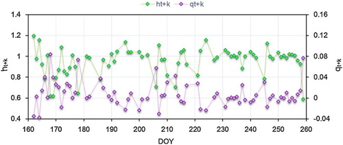
 Figure 5 shows the regression coefficients of the ground-based albedo on each two neighbouring clear-sky days. Most of the slope coefficients ( in Equation (7)) are larger than 0.8 throughout the study period, which meets with the general expectation that the surface albedo values on two neighbouring clear-sky days should be positively correlated with each other. The intercepts ( in Equation (7)) can be thought as the compensation of the linear correlation. Most of the intercepts in the time series are approximately distributed about 0, which indicates that the surface albedos are largely determined by its neighbouring clear-sky days’ surface albedo values.

Figure 5. The OLS regression models’ coefficients between the WSN-based albedos for each two neighbouring clear days.

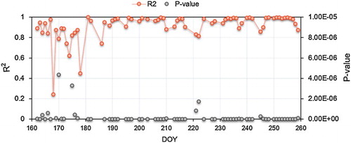
 Figure 6 shows the significance values and determination coefficients of the linear regression models between the ground observed albedos on each two neighbouring clear days. The determination coefficients of the regression models are larger than 0.8 in most cases. In addition, the P values from the F-test are close to 0 for the entire time series. The high R² and low P values indicate significant correlations between the ground observed albedos on each two neighbouring clear-sky days. However, it is noted that the determination coefficient of the regression modelling is low on DOY 168 and DOY 178, which indicates that the surface albedo observations on these two days are not strongly correlated with their neighbouring clear-sky observations. This is because surface albedo values on these two days are substantially different when compared with their neighbouring observations, as shown in Figure 2. However, the construction of the spatiotemporal trend surface is highly dependent on the temporal correlation of the observations made on each two neighbouring clear-sky days in the time series. Thus, only the ground observed albedos after DOY 181 were used in this paper. Based on the regression coefficients between the CASI albedo and ground observed albedo in Figure 4 and the regression coefficients between the ground observed albedos on each two neighbouring clear-sky days in Figure 5, the spatiotemporal trend surface expressed by Equation (8) can be derived.

Figure 6. The R² and significance test results of the OLS regression models between the WSN observed albedo on each two neighbouring clear days.

4.3. Spatiotemporal trend surface evaluation

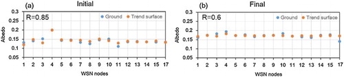
 Figure 7 illustrates the spatial performance of the spatiotemporal trend surface at the locations of the WSN nodes. The trend surface generally agrees with the ground observed values with R of 0.85 and 0.6 on the initial and final days, respectively. For the initial day (DOY 181), the highest albedo measured on a building (node 4) and the lowest albedo measured in a cornfield that had been irrigated (node 11) are both captured by the trend surface. And similar results can be found for the trend surface on the last day of the experimental period. These results demonstrate that the spatiotemporal trend surface can express the spatial pattern of surface albedo over the study area.

Figure 7. The spatial consistency between the trend surface and the ground-based measurements over the WSN nodes. Only the results for the initial and final days are shown for conciseness.

 Figure 8 shows the temporal performance of the spatiotemporal trend surface over the different kinds of land cover types where the WSN nodes were installed. Both the albedo from the trend surface and the ground observed one show similar seasonal variations, and they were quite consistent throughout the period. The trend surface shows the highest correlation, with an R-value of 0.954, with ground-based albedo over cornfields (Figure 8(a)), because most of the WSN nodes (14/17) have been placed on cornfields, and the regression coefficients calculated from the ground-based albedo time series can better depict the temporal variation of cornfields. However, as the highest albedo feature over the study area, the only node on a building also yielded a high R-value of 0.878 (Figure 8(c)), which demonstrates the ability of the spatiotemporal trend surface to capture the temporal characteristics of high albedo land cover during the study period. The node within the vegetable field shows a lower R, with a value of 0.467, than those obtained for cornfields and the building (Figure 8(b)), indicating the inferiority of the trend surface to depict the temporal variation of the vegetable field. Despite the smaller R, the subtle change in the albedo of vegetable field over time can be accurately represented by the spatiotemporal trend surface, as is shown in Figure 8(b). Unfortunately, the node within the orchard is associated with the smallest R, with a value of 0.127, as illustrated in Figure 8(d). This can be attributed to the lowest albedo value of orchard field among different land cover types after DOY 225, as shown in Figure 2.

Figure 8. The temporal consistency between the trend surface and the ground-based measurements over different land cover types during the study period. Only one node within a cornfield is shown for conciseness.

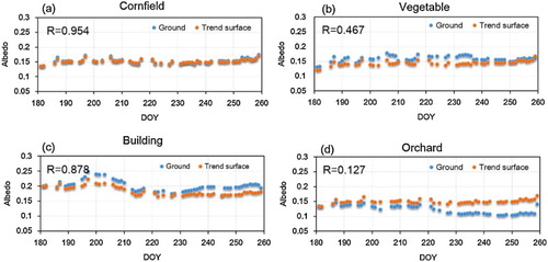
As explained above, the regression coefficients to construct the spatiotemporal trend surface are largely fitted by the albedo values observed over cornfields. Before DOY 225, the albedo values of the orchard are close to that of the cornfields, in terms of both temporal trend and magnitude. Therefore, the spatiotemporal trend surface can describe the magnitude and temporal variation of the orchard well. After DOY 225, however, the albedo of the orchard is always smaller than that of the cornfields and maintains the lowest value among all the WSN nodes’ observations, however, it still had a similar temporal trend as that of the cornfields. Therefore, the value of the trend surface over the orchard deviates from the ground observed one, but the two time series show similar trends. Nevertheless, the slight change in the albedo of the orchard during each small temporal period is accurately captured by the spatiotemporal trend surface. Separating the study period into two parts at DOY 225, the R values increase to 0.47 and 0.51 before and after DOY 225, respectively.

The overall consistency between the trend surface and the ground observed albedo over different land cover types is encouraging, with a high R-value of 0.702. Besides, both the spatial and temporal characteristics of the high albedo values associated with the building and the low albedo values of the cornfields under the influence of occasional irrigation are generally depicted by the spatiotemporal trend surface. The above results demonstrate that the trend surface performs acceptably well in characterizing the spatiotemporal variations in surface albedo.

4.4. Coarse-pixel scale albedo upscaling predictions

 Figure 9 (left) depicts the initial trend surface (DOY 181) and the trend surface on the last clear-sky day (DOY 259) during the study period. The spatial distribution characteristics of the initial trend surface are consistent with the surface features of the study area, as shown in Figure 1. The trend surface indicates relatively high albedo values over buildings, villages and greenhouses, while it shows relatively low albedo values over vegetable fields, orchards, woodlands and cornfields. In particular, cornfields that were watered just before DOY 181 exhibit the lowest albedo values. The initial trend surface exhibits as much details of the spatial pattern as Figure 1, which demonstrates that the initial trend surface can preserve the heterogeneous spatial distribution characteristics of surface albedo.

Figure 9. The trend surface (left) and the upscaling results with a 1-km grid (right) for the initial day (up) and the last clear day (down) during the study period.

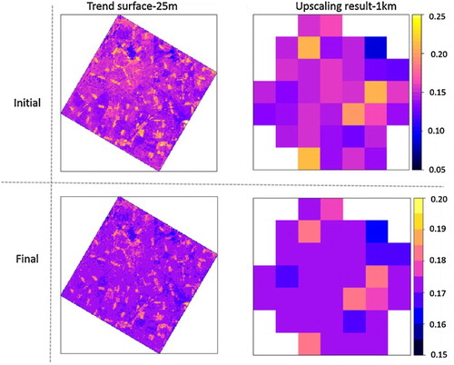
For the trend surface on the final day, the spatial pattern characteristics of surface albedo still hold. The largest values seen in the trend surface still occur over buildings and greenhouses, and these values are distinctly different from those that occur over vegetable fields, orchards, woodlands and cornfields. The scale bars in Figure 9 shows that the trend surface on the final day presents a smaller range of values (0.15–0.2) than that on the initial day (0.05–0.25). In addition, the trend surface values on the final day are generally larger than that on the initial day, with the exception of the values over buildings and orchards. The differences between them are associated with the temporal change in surface albedo over different land cover types due to seasonal variations.

The construction of the spatiotemporal trend surface starts from DOY 181, when the corn and vegetables are seedlings, and when the orchard trees are leafing out. At this stage, the surface albedos show relatively large differences among the different fields, due to differences in growth caused by individual farm management practices. As the time goes on, different land cover types present different temporal trends. The cornfields, as the main land cover, are close with a little gap to the background around DOY 210, which is combined with the decrease in albedo. The cornfields come into maturity with withered cornstalks around DOY 245. Subsequently, the albedo values of the cornfields increase slightly according to the degree of their maturity, resulting in generally higher values of the trend surface on the final clear-sky day. In addition, the cornfield albedo values show smaller differences among the different fields during the final stage of the experiment, as illustrated in Figure 2(b). The vegetable field shows a similar phenology as the cornfields, and its albedo values are very close to those of the cornfields, especially at the end of the experiment (Figure 2(a)). The orchard albedo decreases with time as the leaf area index (LAI) increases. From DOY 230 to the end of the experiment, the LAI reaches its maximum, and its albedo values decrease to their minimum and remain relatively stable (Figure 2(a)). However, it is noteworthy that, on the final clear-sky day, the albedo of the orchard, which has the lowest albedo values within the study area, increases significantly. In contrast, the albedo of the building, which has the highest albedo value among all of the land cover types, decreases. All of these factors contribute to the narrow range of the surface albedo values seen on the final clear-sky day.

It can be concluded that the differences between the trend surfaces on the initial and final clear-sky days correspond to the spatiotemporal characteristics of surface albedo within the study area. This also demonstrates the ability of the spatiotemporal trend surface method to capture the spatiotemporal characteristics of surface albedo over long time series.

Despite the good performance of the spatiotemporal trend surfaces, it should be noted that the trend surfaces over time suffer from the accumulated uncertainties of the regression coefficients in Equation (8). However, this kind of uncertainty can be reduced to some degree by kriging the residuals. After the time series of trend surfaces were constructed, the upscaling predictions over time were derived at a spatial resolution of 1 km (Figure 9 (right)) and a temporal resolution of 1 day using Equation (11).

4.5. Comparison between the upscaled albedo and remote sensing products

For consistency with the temporal composition period of MODIS, GLASS and MuSyQ albedo products, which are 16, 17 and 10 days, the daily upscaling results were first averaged to the temporal step of the albedo products. Scatterplots between the albedo products and the upscaling results within the study area are depicted in Figure 10.

Figure 10. The scatterplots between the upscaling results and albedo products during the study period (from left to right, MODIS (V006), GLASS and MuSyQ).

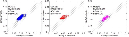
The comparison results of MODIS and MuSyQ with the upscaled albedo predictions are visually similar over the study area. However, the comparison results for the GLASS albedo were remarkably different. In terms of statistical results, the MODIS and MuSyQ albedo products show similarly high accuracies, with small RMSEs near 0.01 and high R² larger than 0.6. Further, the MuSyQ albedo values are closer to the upscaled ground-based albedo values with a smaller mean absolute bias of 0.010, compared with the value of 0.013 for MODIS. The GLASS albedo product has a comparable RMSE of 0.012 and the smallest R² of 0.35 among these three albedo products. The results of this comparison show that the spatiotemporal characteristics of surface albedo can be better depicted by the MODIS and MuSyQ albedo products. The smaller R² and the narrower range of the GLASS albedo product indicate its inferiority in capturing subtle changes in surface albedo in time and space.

The above results are reasonable, considering the characteristics of each albedo product. Based on the BRDF angular modelling adopted for the MODIS albedo product, the MuSyQ albedo algorithm was designed in order to shorten the accumulation period for BRDF/albedo retrievals by combining remote sensing data from multiple sources. As a result, the MuSyQ albedo product features an improved temporal resolution and has an accuracy that is comparable with that of MODIS. In contrast, the GLASS albedo product mainly improves the spatiotemporal continuity of the surface albedo using the STF (Statistics-based Temporal Filtering) algorithm (Liu et al. 2013). The smoothness of the GLASS albedo product leads to the loss of abrupt changes in surface albedo at the same time.

5. Conclusion

Because the validation of coarse-scale albedo products over heterogeneous landscapes suffers from scaling issues, upscaling time series of ground observed albedo is of great importance prior to validation. In this paper, a method for establishing a spatiotemporal trend surface based on limited high-resolution albedo maps has been presented as an effective way to upscale continuous and long-term ground observed albedo to the coarse-pixel scale. This method has been illustrated using WSN-based ground data and a high-resolution CASI image obtained in Heihe River Basin. The evaluation of the spatiotemporal trend surface shows that it can successfully preserve the spatiotemporal characteristics of surface albedo over the study area. By establishing the spatiotemporal trend surface, long time series of ground observed albedo can be upscaled to the coarse-pixel scale and used as reference values to validate three kinds of 1-km albedo products. The validation results indicate that the MODIS (V006) and MuSyQ albedo products are more consistent with the upscaled albedos than the GLASS albedo.

The proposed method is based on the conceptual universal scaling methodology. Compared with traditional multi-scale validation strategy, it permits compensation during the calibration part by applying kriging to the residuals, and it also reduces the impact of the limited time frame of high-resolution albedo maps, thereby enhancing the quality of validation over heterogeneous surfaces. Although this paper investigates the possibility of using ground-observed albedo obtained from WSN observation system for validation of coarse-scale albedo products over heterogeneous surfaces, the proposed method has the potential to be applied to other parameters, such as LAI, soil moisture and sensible heat flux, as long as a network of sampling points and continuous measurements exists.

It should be noted that the construction of the spatiotemporal trend surface depends strongly on the correlations between ground observations made on two neighbouring clear-sky days’. Thus, only the gradual albedo changes can be captured by the proposed method. Since there is only one CASI albedo map available to establish a benchmark for construction of the spatiotemporal trend surface during the study period, only the ground-based measurements after DOY 181 are treated here because of its weakened correlation with the ground-based measurements taken before that day.

When abrupt changes occur on the land surface, the two neighbouring ground observations may not be significantly correlated with each other. In this case, a new albedo map should be introduced to build a new benchmark to establish the trend surface for the following time series. The upscaling procedure in following time series based on the new benchmark can be regarded as a repetition of the current study until the next abrupt change happen. Therefore, the proposed method has the potential to serve for the long-term validation as long as two requirements are satisfied: First, the long time series ground measurements in the form of observation network exists; Second, new high-resolution ancillary image is available when abrupt change happen and the ground measurements between two neighbouring clear-sky days are not significantly correlated.

It is an open issue whether linear regression is sufficient to model the relationship between high-resolution ancillary imagery and ground-based albedo and the relationship between ground observations taken on two neighbouring clear-sky days. We will further validate this method and develop new regression models that are better able to account for the spatiotemporal characteristics of surface albedo in the future.

Acknowledgement

The authors would like to thank all of the scientists, engineers, and students who participated in the HiWATER campaigns, which provided airborne products and WSN data products for this work.

Disclosure statement

No potential conflict of interest was reported by the authors.

Additional information

Funding

This research is jointly supported by the National Basic Research Program of China [grant number 2013CB733401], the National Natural Science Foundation of China [grant numbers 41671363 and 91125003].

References

- Camacho, F., J. Cernicharo, R. Lacaze, F. Baret, and M. Weiss. 2013. “GEOV1: LAI, FAPAR Essential Climate Variables and FCOVER Global Time Series Capitalizing Over Existing Products. Part 2: Validation and Intercomparison with Reference Products.” Remote Sensing of Environment 137: 310–329. doi: 10.1016/j.rse.2013.02.030
- Chen, Y. M., S. Liang, J. Wang, H. Y. Kim, and J. V. Martonchik. 2008. “Validation of MISR Land Surface Broadband Albedo.” International Journal of Remote Sensing 29 (23): 6971–6983. doi: 10.1080/01431160802199876
- Crow, W. T., A. A. Berg, M. H. Cosh, A. Loew, B. P. Mohanty, R. Panciera, P. Rosnay, D. Ryu, and J. P. Walker. 2012. “Upscaling Sparse Ground-Based Soil Moisture Observations for the Validation of Coarse-Resolution Satellite Soil Moisture Products.” Reviews of Geophysics 50 (2): 3881–3888. doi: 10.1029/2011RG000372
- Dickinson, R. E. 1995. “Land Processes in Climate Models.” Remote Sensing of Environment 51: 27–38. doi: 10.1016/0034-4257(94)00062-R
- Ge, Y., Y. Liang, J. Wang, Q. Zhao, and S. Liu. 2015. “Upscaling Sensible Heat Fluxes with Area-to-Area Regression Kriging.” IEEE Geoscience and Remote Sensing Letters 12 (3): 656–660. doi: 10.1109/LGRS.2014.2355871
- Hengl, T., G. B. Heuvelink, and D. G. Rossiter. 2007. “About Regression-Kriging: From Equations to Case Studies.” Computers & Geosciences 33 (10): 1301–1315. doi: 10.1016/j.cageo.2007.05.001
- Jin, Y., C. B. Schaaf, C. E. Woodcock, F. Gao, X. W. Li, A. H. Strahler, W. Lucht, and S. L. Liang. 2003. “Consistency of MODIS Surface Bidirectional Reflectance Distribution Function and Albedo Retrievals: 2. Validation.” Journal of Geophysical Research: Atmospheres (1984–2012) 108 (D5): 4159. doi: 10.1029/2002JD002804
- Kang, J., R. Jin, and X. Li. 2015. “Regression Kriging-Based Upscaling of Soil Moisture Measurements from a Wireless Sensor Network and Multiresource Remote Sensing Information Over Heterogeneous Cropland.” IEEE Geoscience and Remote Sensing Letters 12 (1): 92–96. doi: 10.1109/LGRS.2014.2326775
- Kotchenova, S. Y., E. F. Vermote, R. Matarrese, and F. J. Klemn. 2006. “Validation of a Vector Version of the 6S Radiative Transfer Code for Atmospheric Correction of Satellite Data. Part I: Path Radiance.” Applied Optics 45 (26): 6762–6774. doi: 10.1364/AO.45.006762
- Li, X., G. Cheng, S. Liu, Q. Xiao, M. Ma, R. Jin, T. Che, Q. Liu, W. Wang, and Y. Qi. 2013. “Heihe Watershed Allied Telemetry Experimental Research (HiWATER): Scientific Objectives and Experimental Design.” Bulletin of the American Meteorological Society 94: 1145–1160. doi: 10.1175/BAMS-D-12-00154.1
- Liang, S. 2001. “Narrowband to Broadband Conversions of Land Surface Albedo. I. Algorithms.” Remote Sensing of Environment 76: 213–238. doi: 10.1016/S0034-4257(00)00205-4
- Liang, S. 2003. “A Direct Algorithm for Estimating Land Surface Broadband Albedos from MODIS Imagery.” Geoscience and Remote Sensing, IEEE Transactions on 41: 136–145. doi: 10.1109/TGRS.2002.807751
- Liang, S. 2005. Quantitative Remote Sensing of Land Surfaces. New York: Wiley.
- Liang, S., H. Fang, M. Z. Chen, C. J. Shuey, C. Walthall, C. Daughtry, J. Morisette, C. Schaaf, and A. Strahler. 2002. “Validating MODIS Land Surface Reflectance and Albedo Products: Methods and Preliminary Results.” Remote Sensing of Environment 83 (1): 149–162. doi: 10.1016/S0034-4257(02)00092-5
- Liu, N. F., Q. Liu, L. Z. Wang, S. L. Liang, J. G. Wen, Y. Qu, and S. H. Liu. 2013. “A Statistics-Based Temporal Filter Algorithm to map Spatiotemporally Continuous Shortwave Albedo From MODIS Data.” Hydrology & Earth System Sciences 17 (6): 2121–2129. doi: 10.5194/hess-17-2121-2013
- Liu, J. C., S. Schaaf, A. Strahler, Z. T. Jiao, Y. M. Shuai, Q. L. Zhang, M. Román, J. A. Augustine, and E. G. Dutton. 2009. “Validation of Moderate Resolution Imaging Spectroradiometer (MODIS) Albedo Retrieval Algorithm: Dependence of Albedo on Solar Zenith Angle.” Journal of Geophysical Research 114: D01106. doi: 10.1029/2008JD010805
- Liu, S. M., Z. W. Xu, L. S. Song, Q. Y. Zhao, Y. Ge, T. R. Xu, Y. F. Ma, Z. L. Zhu, Z. Z. Jia, and F. Zhang. 2016. “Upscaling Evapotranspiration Measurements from Multi-Site to the Satellite Pixel Scale Over Heterogeneous Land Surfaces.” Agricultural and Forest Meteorology 230–231: 97–113. doi: 10.1016/j.agrformet.2016.04.008
- Lucht, W., C. B. Schaaf, and A. H. Strahler. 2000. “An Algorithm for the Retrieval of Albedo from Space Using Semiempirical BRDF Models.” IEEE Transactions on Geoscience and Remote Sensing 38: 977–998. doi: 10.1109/36.841980
- Mira, M., M. Weiss, F. Baret, D. Courault, O. Hagolle, and B. Gallego-Elvira. 2015. “The Modis (Collection v006) Brdf/Albedo Product mcd43d: Temporal Course Evaluated Over Agricultural Landscape.” Remote Sensing of Environment 170: 216–228. doi: 10.1016/j.rse.2015.09.021
- Peng, J. J., Q. Liu, J. G. Wen, Q. H. Liu, Y. Tang, L. Z. Wang, B. C. Dou, et al. 2014. “Multi-scale Validation Strategy for Satellite Albedo Products and its Uncertainty Analysis.” Science China: Earth Sciences 58: 573–588. doi: 10.1007/s11430-014-4997-y
- Qu, Y., Q. Liu, S. L. Liang, L. Z. Wang, N. F. Liu, and S. H. Liu. 2014. “Direct-estimation Algorithm for Mapping Daily Land-Surface Broadband Albedo from MODIS Data.” IEEE Transactions on Geoscience and Remote Sensing 52 (2): 907–919. doi: 10.1109/TGRS.2013.2245670
- Román, M. O., C. K. Gatebe, and Y. Shuai. 2013. “Use of In Situ and Airborne Multiangle Data to Assess MODIS-and Landsat-Based Estimates of Directional Reflectance and Albedo.” IEEE Transactions on Geoscience and Remote Sensing 51: 1393–1404. doi: 10.1109/TGRS.2013.2243457
- Sailor, D. J., K. Resh, and D. Segura. 2006. “Field Measurement of Albedo for Limited Extent Test Surfaces.” Solar Energy 80: 589–599. doi: 10.1016/j.solener.2005.03.012
- Schaaf, C. B., F. Gao, A. H. Strahler, W. Lucht, X. Li, T. Tsang, N. C. Strugnell, et al. 2002. “First Operational BRDF, Albedo, Nadir Reflectance Products from MODIS.” Remote Sensing of Environment 83: 135–148. doi: 10.1016/S0034-4257(02)00091-3
- Souza, R. B., M. M. Mata, C. A. E. Garcia, M. Kampel, E. N. Oliveira, and J. A. Lorenzzetti. 2006. “Multi-Sensor Satellite and in Situ Measurements of a Warm Core Ocean Eddy South of the Brazil–Malvinas Confluence Region.” Remote Sensing of Environment 100: 52–66. doi: 10.1016/j.rse.2005.09.018
- Stroeve, J., J. E. Box, F. Gao, S. Liang, A. Nolin, and C. Schaaf. 2005. “Accuracy Assessment of the MODIS 16-day Albedo Product for Snow: Comparisons with Greenland In Situ Measurements.” Remote Sensing of Environment 94: 46–60. doi: 10.1016/j.rse.2004.09.001
- Stroeve, J., J. E. Box, Z. S. Wang, C. Schaaf, and A. Barrett. 2013. “Re-evaluation of MODIS MCD43 Greenland Albedo Accuracy and Trends.” Remote Sensing of Environment 138: 199–214. doi: 10.1016/j.rse.2013.07.023
- Vermote, E. F., N. El Saleous, C. O. Justice, Y. J. Kaufman, and J. L. Privette. 1997. “Atmospheric Correction of Visible to Middle-Infrared EOS-MODIS Data Over Land Surfaces: Background, Operational Algorithm and Validation.” Journal of Geophysical Research: Atmospheres (1984–2012) 102 (D14): 17131–17141. doi: 10.1029/97JD00201
- Wang, K., S. Liang, C. L. Schaaf, and A. H. Strahler. 2010. “Evaluation of Moderate Resolution Imaging Spectroradiometer Land Surface Visible and Shortwave Albedo Products at FLUXNET Sites.” Journal of Geophysical Research 115 (D17): D17107. doi: 10.1029/2009JD013101
- Wang, K., J. Liu, X. Zhou, M. Sparrow, M. Ma, Z. Sun, and W. Jiang. 2004. “Validation of the MODIS Global Land Surface Albedo Product Using Ground Measurements in a Semidesert Region on the Tibetan Plateau.” Journal of Geophysical Research 109: D05107. doi:10.1029/2003JD004229.
- Wang, Y., D. Xie, and X. Li. 2014. “Universal Scaling Methodology in Remote Sensing Science by Constructing Geographic Trend Surface.” Journal of Remote Sensing 18 (6): 1139–1146.
- Wen, J. G., B. C. Dou, D. Q. You, Y. Tang, Q. Xiao, and Q. H. Liu. 2016. “Forward a Small-Time Scale BRDF/Albedo by Multi-Sensors Combined BRDF Inversion (MCBI) Model.” IEEE Transaction on GeoScience and Remote Sensing. doi:10.1109/TGRS.2016.2613899.
- Wen, J. G., Q. H. Liu, L. Qiang, Q. Xiao, and X. W. Li. 2009. “Parametrized Brdf for Atmospheric and Topographic Correction and Albedo Estimation in Jiangxi Rugged Terrain, China.” International Journal of Remote Sensing 30 (11): 2875–2896. doi: 10.1080/01431160802558618
- Wu, X., Q. Xiao, J. Wen, Q. Liu, D. You, and B. Dou. 2016. “Upscaling In Situ Albedo for Validation of Coarse Scale Albedo Product Over Heterogeneous Surfaces.” International Journal of Digital Earth 1–19.
- Xu, Z., S. Liu, X. Li, S. Shi, J. Wang, Z. Zhu, and M. Ma. 2013. “Intercomparison of Surface Energy Flux Measurement Systems Used During the HiWATER-MUSOEXE.” Journal of Geophysical Research: Atmospheres 118 (23): 13–140.
- You, D., J. G. Wen, Q. Xiao, Q. Liu, J. J. Peng, Q. H. Liu, Y. Tang, and B. C. Dou. 2015. “Development of a High Resolution BRDF/Albedo Product by Fusing Airborne CASI Reflectance with MODIS Daily Reflectance in the Oasis Area of the Heihe River Basin, China.” Remote Sensing 7: 6784–6807. doi: 10.3390/rs70606784