Speckle filtering of Synthetic Aperture Radar images using filters with object-size-adapted windows

ABSTRACT

Speckle degrades the radiometric quality of a Synthetic Aperture Radar (SAR) image. Previous methods for speckle reduction have used a fixed-size window for filtering the entire image. This, however, may not be effective for the entire image, as land covers of different sizes require different filtering windows. In this paper, a novel method is proposed by which each pixel in the image is filtered with a window appropriate for the size of object within it. The real in-phase and the imaginary quadrature components of the SAR images determine the best window size and the pixels in the intensity image are filtered using their own optimal windows. The proposed method is presented for both single- and multi-polarized SAR images, and the results of several common filters that were modified are presented. This approach is applied to two RADARSAT-2 images: one over San Francisco, California, USA and the other over St. John’s, Newfoundland and Labrador, Canada, producing results that were similar to, or outperformed, comparable filters while retaining details and suppressing speckle effectively. While the method was successful for single-look intensity data, it offers great potential for multi-look and amplitude data as well.

KEYWORDS:

• Speckle
• Synthetic Aperture Radar (SAR)
• filters
• adaptive window size

1. Introduction

Synthetic Aperture Radar (SAR) images are valuable assets for various applications because of their all-weather and day and night acquisition capability. However, these valuable resources are blemished with the presence of speckle. An intrinsic feature of SAR images, speckle originates from the coherently recorded pulses returning from the earth surface. Speckle degrades the radiometric quality of the image, thus hindering image interpretation and reducing the accuracy of image segmentation and classification (Lee and Pottier 2009). Consequently, since the advent of SAR images, there has been a host of studies addressing the issue of speckle reduction. Early on, starting from a study by Lee (1980), it was understood that the typical techniques applied for image noise suppression are not effective for SAR images. Lee’s research proposed filters that exploit local statistics of the image, namely adaptive filters. He suggested that speckle acts as multiplicative noise and, based on that, he proposed a filter by minimizing the mean square error. The filter was known as the MMSE filter (Lee 1980, 1981b) and became the basis of many other algorithms. The MMSE filter, however, fails to suppress speckle effectively close to edges (Lee and Pottier 2009), and hence Lee refined it by using edge-aligned, non-square windows (1981a). He also proposed the sigma filter (Lee 1983a, 1983b) based on the sigma probability of a Gaussian distribution. As sigma filter was insufficient in maintaining strong targets and produced biased estimation, an improved version of that was proposed in Lee et al. (2009). Besides Lee’s filters, other similar techniques were proposed for speckle reduction in single-band SAR images while preserving image sharpness. Frost et al. (1981, 1982) calculated the impulse response of the filter by solving the MMSE problem using a different error measure. Kuan et al. (1985) also dealt with the MMSE problem and reached the same general form as Lee (1980), but with a different weight function for balancing the role of pixel reflectance and that of the local statistics.

In subsequent years, single-band SAR filters were further improved. Lopes, Touzi, and Nezry (1990) noted that there are different regions in a SAR image, namely homogeneous, heterogeneous, and point targets. He stated that speckle should not be reduced by the same amount in the three different regions, and suggested measures for distinguishing among the three different areas. He modified the commonly used filters based on his idea. A few years later, in 1993, Lopes et al. (1993) also proposed a filter which was known as the Gamma filter, in which homogeneous regions, edges, lines, and point targets are detected using more robust measures. There have also been a few other innovative studies. In Park, Song, and Pearlman (1999), for example, a method was proposed for filtering which exploited local statistics to change the filtering window in a range. A growing regional method based on a statistical measure was applied for selection of window sizes in an approach suggested in Nicolas, Tupin, and Maître (2001). Other filtering algorithms that have been proposed include Datcu, Seidel, and Walessa (1998), Walessa and Datcu (2000), and Kuan et al. (1987). A more comprehensive review can be found in Durand, Gimonet, and Perbos (1987), Lee et al. (1994), and Touzi (2002).

With the advancement of SAR sensors, Polarimetric SAR (PolSAR) images became available, and this development was followed by the need for filters for PolSAR images. Novak and Burl (1990) pioneered in this field by developing the polarimetric whitening filter (PWF). In the PWF, all elements of the scattering matrix are combined optimally to form a single, speckle-reduced image. In Lee, Grunes, and Mango (1991), the MMSE filter was extended to the diagonal elements of the covariance matrix, but the off-diagonal elements were ignored. While speckle for the diagonal terms can be modelled as multiplicative noise, a multiplicative noise model is not effective for off-diagonal terms. Consequently, off-diagonal terms should be modelled by a combination of multiplicative and additive noise (Lee and Pottier 2009). Goze and Lopes (1993) continued Lee’s work by MMSE filtering of all terms in the covariance matrix. Lopes and Séry (1997) developed another filter for PolSAR data focusing on image texture. Lee et al. (2003) suggested a filter useful for interferometric applications in forested areas. Lee et al. (2015) also extended the improved single-band sigma filter to PolSAR data. In the proposed filter, the authors attempted to maintain the strong point targets and to preserve the scattering mechanisms. However, preliminary attempts for speckle filtering in PolSAR images fail to preserve polarimetric features, that is, they introduce cross-talk between channels and/or alter the cross-correlation between bands, although they can be useful in some applications such as target detection (Lee and Pottier 2009). Therefore, polarimetric filters such as those used in Lee, Grunes, and De Grandi (1999) and Lee et al. (2006) were proposed to maintain polarimetric information. In polarimetric filters, all elements of the covariance matrix are filtered by the same amount and in the same way, and the filtering is performed independently on each term to avoid cross-talk, that is, altering correlation between channels.

In recent years, some other valuable works have been also proposed on speckle reduction. For example, in Lang, Yang, and Li (2015), a three-step filter was proposed for speckle reduction in SAR images. First, the authors developed a line and edge detector, based on which they defined a homogeneity measure. Subsequently, they exploited the homogeneity measure to adjust the shape and size of filtering, and obtained promising results. Moreover, in Torres et al. (2014), a speckle filtering approach was proposed that exploits the non-local means and stochastic distances to reduce speckle. Deledalle, Tupin, and Denis (2010), Deledalle, Denis, and Tupin (2011), and Chen et al. (2011) also proposed non-local approaches for speckle reduction. Non-local filters define the weights based on the distance between the reference patch and similar neighbouring patches (Argenti et al. 2013).

Although the speckle reduction methods described in the publications reviewed above perform reasonably well both in single-band and multi-polarized cases, selection of window size is almost always a challenging task. In fact, choosing a fixed window size for filtering the entire image has a proper outcome only if all the targets in the image are of the same size, which is not a valid assumption for most real-world images. Thus, as the weights of the filtering window for each pixel are adaptive, the window size should also be adaptive. The main objective of this paper is to introduce a method for automatically selecting the filtering window size for each pixel. This approach is presented in both single-band and multi-polarized versions. Common filtering methods such as the box-car and MMSE filters have been adjusted using our proposed adaptive window size approach and the results are presented.

This paper has been organized as follows: in Section 2, the method is presented in terms of single-band and multi-polarized data. Section 3 includes a description of the data sets and study areas. In Section 4, filtered images are investigated and some numerical indices are introduced for the assessment. Discussion of the results is the topic of Section 5, and finally, Section 6 includes concluding remarks.

2. Method

When working with SAR images, it is the real value of the backscatter coefficient that is of interest. For distributed targets, this value is altered by the effect of interference (Oliver and Quegan 2004). The aim of speckle filtering is therefore to average the returned values from all the scatterers which contribute to the same distributed target in order to achieve a more accurate estimation of the backscattering coefficient. For this task, a fixed-sized rectangular window is not effective for several reasons. First, the actual shape of a target might not be rectangular. Thus, a rectangular window includes either fewer or more scatterers than the correct number which causes the estimated backscattering coefficient to be inaccurate. The defect can be observed by noting the smeared boundaries of the target near its edges. Second, not all the distributed targets in an image are of the same size. Hence, a window size which can be appropriate for one part of the image might not be applicable for the targets in another part.

The first problem has been addressed extensively in the literature and much of it was mentioned in Section 1. Different adaptive filters have been introduced to exploit the local statistics in an attempt to include only the scatterers from the same target in the filtering process over that target. The second issue, however, has not been investigated as much as the first one. The main objective of this paper is to address this issue.

2.1. Average filtering of single-band SAR data with adaptive window size

Speckle can be regarded as the fluctuation of pixel values around a mean which is the desired backscattering coefficient of the target (Oliver and Quegan 2004). Naturally, the best possible estimation of the true mean is achieved when all the scatterers from the target are involved in the averaging process, and no scatterer from another neighbouring object is included in filtering. This is the definition which can specify the best filtering window for each pixel within the target as will be presented below.

Although in practice there is correlation between the neighbouring pixels of a SAR image (Lee and Pottier 2009), in principle, each sample (resolution cell) in a target, here referred to as A, can be considered as an independent observation for estimating the true backscattering coefficient of target A. Thus, a rectangular window which lies entirely within the target includes n independent observations:(1) In Equation (1), is an arbitrary parameter, which can be considered the real backscattering coefficient of the target in this context. is the parameter to be estimated from n observations, which is the backscattering coefficient estimated from resolution cells. is the ith observation made for estimating which is assumed to be the pixel value of a SAR image. SAR images are provided in different formats: real and imaginary (in-phase and quadrature, respectively), amplitude and phase, and intensity images (Oliver and Quegan 2004). We assume that n observations are in real and imaginary format indicating that the pixel value consists of in-phase and quadrature components, that is:(2) where . It has been shown that the real and imaginary components in SAR images, when considered individually, tend to have a normal distribution (Oliver and Quegan 2004). For normally distributed data, the mean is an efficient estimator (Korostelev and Korosteleva 2011). This means that if is the average of the real or imaginary part of the observations, that is:(3) Then, considering as a random variable, pixels result in a smaller standard deviation than pixels, and a greater standard deviation than pixels (Therrien and Tummala 2011). This means that if the window containing the observations to be averaged grows larger, the standard deviation will tend to decrease until the window also begins to contain outliers, that is, observations from other targets. Therefore, the window which yields the minimum value for standard deviation will include a maximum number of observations from target A, but a minimum of observations from neighbouring objects. It should be noted, however, that while is used to assign the optimal window size for each pixel, it cannot be applied for speckle reduction, since averaging real or imaginary data individually does not convey any useful information for SAR data analysis. In fact, averaging them is a coherent vector summation and has no effect on speckle reduction (Lee and Pottier 2009), while for speckle reduction, an incoherent summation is needed. Consequently, while the real and imaginary data are exploited for the determination of the best window size for each pixel, it is the intensity image that is to be used for averaging the samples using that optimal window size.

Figure 1 schematically shows the standard deviation of pixels (either from the real or from the imaginary part of the image) with different window sizes. The smallest window contains limited pixels from target A which have standard deviation . With the explanation above, it is expected that as the number of samples for computation of the average increases, the value of standard deviation will decrease. This reduction continues until the window begins to overlap pixels of adjacent objects. Once the window contains pixels from two different objects, the standard deviation will tend to increase. Thus, the optimum window size is the one which corresponds to the minimum standard deviation, computed using the real or imaginary components of the samples in the window. Then, this window size is used in the intensity image to reduce speckle of the pixel at the centre of the window. Based upon the above discussion, the filtering process can be outlined as follows:

1. A range of window sizes is selected by investigating the SAR image. This range must contain appropriate filtering sizes for all the objects of the image, from the smallest target to the largest. An appropriate range of window sizes can be 3–21.

2. Both the real and imaginary parts of the image are averaged separately using the windows covering the entire range of sizes, thus computing the standard deviation corresponding to each window in the size range for all pixels.

3. The appropriate filter size for each pixel is selected as the one which corresponds to the minimum standard deviation for that pixel over the whole range of standard deviations (i.e. window sizes). If the optimal size obtained from the real and imaginary parts is different for any pixel, their average is considered as the optimal window size. When the standard deviation monotonically increases, this means that there is likely a point target in the image with a high amount of backscatter, and likely the best window size for filtering is the smallest. A monotonic decrease in standard deviation indicates that the area is likely completely homogeneous, and the largest window size is the best. In the events of two minimums, it is probable that the first minimum has occurred when all the samples from the first target have been taken into account and the second minimum has likely occurred when all the samples from the first targets and the other neighbouring (and similar) target(s) have been considered. Therefore, the first minimum standard deviation is the best choice.

4. Using a common method, a speckle-reduced intensity image is acquired by filtering each pixel with its corresponding optimal window. The simplest method is obviously averaging, which is the topic of this section. Other common methods, however, can also be used and will be elaborated.

Figure 1. The samples contained in the smallest window have the standard deviation . As the window grows larger, the standard deviation decreases until it overlaps pixel(s) from the adjacent object(s).

These steps are schematically illustrated in Figure 2.

Figure 2. Flow chart of the proposed algorithm, filtering with adaptive window size.

2.2. MMSE filtering of single-band SAR data with adaptive window size

Figure 1 shows the ideal case, that is, when the pixel to be filtered is almost in the centre of the target. Apart from that, especially for the pixels near the edge of the target (see Figure 3), average filter with adaptive window size might not perform best, a common problem of a simple averaging filter. The proposed method, therefore, can be combined with the MMSE filter (Lee 1980) in order to solve this problem.

Figure 3. Near the edges of a target, the average filter with adaptive window size is not expected to work effectively. This is because as the filtering window overlaps parts of other targets before the window size becomes large enough to provide an accurate estimate of the backscattering coefficient.

2.2.1. Review of the MMSE filter

The MMSE filter, proposed by Lee (1980), has the following form:(4) In Equation (4), is the estimated intensity of the pixel , is the observed intensity for the pixel (x,y), and is the average intensity in a local window. is a weight parameter which is computed by the following formula (obtained by the concept of MMSE):(5) where is the variance of the intensity in the local window and(6) is a characteristic of speckle which is the ratio of the standard deviation to the mean in a homogeneous area; its value for single-look SAR data is 1 (Lee 1986).

2.2.2. The proposed method

The weight parameter in Equation (5) will tend to be small in homogeneous regions and large in heterogeneous regions. Therefore, according to Equation (4), when using square-shaped windows, the role of the local mean is minor when filtering the pixels near edges, while it is significant when the central pixel is located around the middle of the target. The local statistics in the Lee filter of Equation (4) are traditionally computed in a window of fixed size. However, in Equation (4) can be replaced with the optimal mean value computed over the optimal window for each pixel as described in the previous section. Moreover, in Equation (5) can be replaced by the variance of the values included in the optimal window. By making these two changes, the MMSE filter with adaptive window size is obtained.

2.3. Average filtering of PolSAR data with adaptive window size

A full-polarimetric radar sensor records a scattering matrix of each target which is defined as below:(7) where for each term , , and represent transmitted and received polarizations, respectively. Using a well-known result in Boerner et al. (1998), for monostatic SAR and hence, the target can be characterized entirely by the 3-D Lexicographic feature vector:(8) where superscript T denotes matrix transpose. Then the polarimetric covariance matrix and its span (total power) can be obtained using the target vector with Equations (9) and (10), respectively; that is.(9) (10)

where the superscript * represents the complex conjugate. A filter must have the following characteristics to preserve polarimetric features and be known as a ‘polarimetric’ filter (Lee, Grunes, and De Grandi 1999):

1. All terms of the covariance matrix must be filtered in the same way and by the same amount;

2. Each term of the covariance matrix must be filtered independently to avoid cross-talk between polarization channels;

3. The filtering should be adaptive so that scattering characteristics are maintained.

The simplest way for filtering polarimetric images is to average the neighbouring covariance matrices in a window of specific size. Although this filter is not adaptive, it preserves polarimetric features and the correlation between channels, and can be adequate for some applications (Lee and Pottier 2009).

The idea proposed for using adaptive window sizes is extendable to the average filtering of covariance matrices. The feature vector in Equation (8) contains three real and three imaginary components from the three polarimetric channels. For the polarimetric case, all six components can be used to select the optimum window size for each pixel following the same procedure as described in Section 2.1, since the definition of target is the same in all bands, even if they might appear visually different in each band. If the optimal window sizes obtained from six images differ from each other, their average is used as the best window size. Then, the covariance matrices in the window selected for each pixel are averaged to form the speckle-reduced matrix for that pixel.

2.4. Polarimetric filtering of SAR data with adaptive window size

Lee, Grunes, and De Grandi (1999) extended his refined filter (Lee 1981a) to PolSAR data. Let Z be the covariance matrix of the pixel to be filtered. Then, the filtered covariance matrix, , can be estimated by the following expression (Lee, Grunes, and De Grandi 1999):(11) In Equation (11), is the average of the covariance matrices in a non-square, edge-aligned window chosen using the span image (see Lee, Grunes, and De Grandi (1999) for more details), and W is the same weight parameter in Equation (4).

In this paper, six real and imaginary images for all three channels are used for computing the optimal window as described in Section 2.1, and the obtained size per pixel from each image is averaged to achieve the final optimal size. Then, W is computed from the span image in the optimal window. After that, Equation (11) is applied to estimate the speckle-reduced polarimetric covariance matrix for each pixel.

3. Data set and study areas

For testing the performance of our algorithm, two separate data sets were selected. The first one is a RADARSAT-2 full-polarimetric image over San Francisco, California, USA located at approximately 37° 45′ and 122° 26′ W This image was acquired in FQ9 beam mode and Single Look Complex (SLC) format in 2008. This area contains divergent land covers such as vegetation, ocean, and built-up areas, and has long been used for testing the performance of different SAR speckle-reducing filters. The selected subset in the entire image is illustrated in Figure 4(A).

Figure 4. The selected subsets for applying the suggested filters: (A) San Francisco and (B) St. John’s.

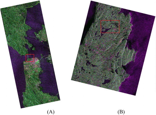
For the purpose of illustrating the robustness of the algorithm, the proposed filters were also applied to another image. This RADARSAT-2 full-polarimetric image was acquired in 2015 over the Avalon Peninsula near St. John’s, Newfoundland and Labrador, Canada, at approximately 47° 33′ and 52° 32′, in FQ4 beam mode and SLC format. This image also covers natural, urban (including an international airport), and ocean areas. The study area specified in the whole image is displayed in Figure 4(B).

For a more precise visual inspection, a Google Earth^TM image from San Francisco, and a 2008 very high resolution (VHR) image from Avalon Peninsula have also been used. For the purpose of emphasizing the details, in this paper, the results of the filters have been shown on selected sub-images. All odd numbers between and including 3 and 21 were considered as the range of window sizes to be applied on the images. This range was selected by visual inspection of both images.

4. Results

4.1. Single-band case

For single-band case, the proposed method was applied on both simulated and real SAR images. The obtained results along with their validation are presented in the following sections.

4.1.1. Simulated SAR image

In order to evaluate the performance of the proposed method, simulated images with and without speckle were applied. Here, the simulated, without speckle images are referred to as the ground-truth images. The simulation procedure of the speckled images is illustrated in Figure 5. As mentioned before, the real and imaginary parts of a SAR image have normal distribution with mean of zero and variance of where is the backscattering coefficient (Lee and Pottier 2009). This fact can be used for simulation of an arbitrary SAR image. Therefore, two classes with a given were considered and the real and imaginary components of the SAR images were created using a normal distribution with mean of zero and variance of . Then, the intensity images were generated by combining the components to simulate a one-look SAR image (Figure 5).

Figure 5. The block diagram of the simulation method.

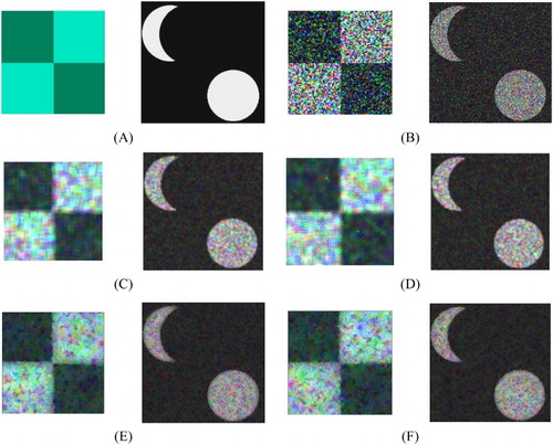
 Figure 6 shows the result of simulation. The left simulated SAR image shows a region containing two different classes, and the right simulated SAR image illustrates two objects within a clutter (Oliver and Quegan 2004). Different filters, including the proposed ones, were applied to these two images and the performance of those filters was evaluated using with-reference indices. The details are presented below.

Figure 6. Simulated SAR images: (A) the ground-truth images, (B) the original intensity images, (C) the 5 × 5 average filtered images, (D) the 5 × 5 MMSE (Lee 1980, 1981a) filtered images, (E) average filtered images with adaptive window size, and (F) MMSE filtered images with adaptive window size.

Figure 6 shows the ground-truth and speckled images, and despeckled images using average and MMSE filters with both fixed and adaptive window sizes. The intensity images, shown in Figure 6(B) are severely contaminated with speckle. Average filter almost suppressed speckle effectively, but the borders are blurred. MMSE filter had a better performance in maintaining the boundaries. Some brighter, isolated points, however, can be seen in the image. Average and MMSE filters with adaptive window size were effective in suppressing speckle while efficiently preserving the boundaries.

Evaluation of the performance of different filters can also be done using with-reference indices. One of the most well-known ones is mean square error (MSE), which is defined as below:(12) where and are despeckled and ground-truth images, respectively. Another useful measure is signal-to-noise ratio (SNR) which is shown in Equation (13):(13) where is the ground-truth image.

As MSE and SNR are for evaluation of the general performance of a filter (Argenti et al. 2013), Structural Similarity Index Measurement (SSIM) (Wang et al. 2004) can be used for estimating the amount of feature preservation in the image. This index is defined as:(14) where and are suitable constants which were chosen as 0.01 and 0.03 in this work. Moreover, and are the ground-truth and despeckled images, respectively.

The three above-mentioned indices were computed for images filtered by the 5-by-5 average and MMSE (Lee 1980) filters (for the sake of comparison) and their adaptive window size counterparts and the results are shown in Table 1. MSE is smaller for the fixed-size average and MMSE filters than their adaptive-size counterparts which in turn causes SNR to be larger for them. This means that the fixed-size filters introduced less bias to the image compared to the proposed ones. SSIM, however, is almost the same for all filters which shows that the filters had similarly retained the structures.

Table 1. Various indices for evaluation and comparison of the performance of the proposed speckle filters on the simulated SAR images.

	MSE		SNR		SSIM
	1st Image	2nd Image	1st Image	2nd Image	1st Image	2nd Image
Average filter	0.0537	0.0556	−1.2773	−3.3865	0.7086	0.6503
MMSE filter (Lee 1980, 1981a)	0.0565	0.0567	−1.5007	−3.4727	0.6905	0.6408
Average filter with adaptive window size	0.0815	0.0686	−3.0921	−4.2946	0.6519	0.6208
MMSE filter with adaptive window size	0.0813	0.0685	−3.0775	−4.2894	0.6429	0.6151

It should be noted that the result of filtering on the synthetically speckled SAR images is not enough for drawing conclusions about performance of filters on real SAR images (Argenti et al. 2013), because the selected ground-truth image and the real ground-truth reflectivity can differ significantly (Argenti et al. 2013). Moreover, a simulated SAR image cannot be consistent with a real SAR image in terms of image formation and acquisition process (Argenti et al. 2013). Therefore, the experiment should be done on real SAR images as well.

4.1.2. Real SAR image

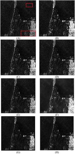
For the implementation of the single-band version of the method, the HH channel was selected from both full-polarimetric images introduced in Section 3. For comparison, the average, MMSE (Lee 1980), enhanced Lee filter (Lopes, Touzi, and Nezry 1990), and Gamma filter (Lopes et al. 1993) with a fixed window size (5 × 5 window), and a non-local filter, the probabilistic patch-based filter (PPB; Deledalle, Denis, and Tupin 2009), were also applied to the image. The PPB filter has various user-defined parameters, namely half sizes of the search window width, half sizes of the window width, and number of iterations, and the value of each is described in the figure caption corresponding to both study area. Figure 7 illustrates the results for a sub-image of the San Francisco area. The original one-look HH intensity image is blemished with the effect of speckle. Although the 5 × 5 average filter has improved the images visually in homogeneous regions, boundaries and subtle objects are smeared. The MMSE filter outperformed the average filter in retaining the edges and details; a fair amount of speckle, however, is still present in the image and occasional isolated pixels with higher intensity can be viewed in homogeneous regions. The enhanced Lee filter preserved even more details. However, in some parts, for example, the urban area in the bottom right of the image, the objects seem rather noisy and have not been evenly filtered. Moreover, isolated points, that is, the points brighter than their surrounding parts, are still present in the image. The Gamma filter had almost the same performance as the enhanced Lee filter, with isolated points being present sporadically. In addition, the objects in urban areas are also not completely clear in the filtered image. It should be noted that in practice, usually larger window sizes are used for filtering, which causes more blurring. The PPB filter effectively reduced speckle although the urban area was slightly blurred. The proposed average filter with adaptive window size shows a significant improvement, both by suppressing speckle in homogeneous areas and maintaining the object boundaries. Some details, however, are blurred as a result of over-filtering. This downside is not observed in the proposed MMSE filter with adaptive window size. The result using adaptive window size shows that details were well preserved as seen in Figure 7(E,F), while speckle was successfully suppressed in homogenous regions.

Figure 7. San Francisco: (A) original one-look HH intensity image. The rectangle on the top and the bottom of the image show the regions used for computation of ENL and coefficient of variation, respectively, (B) the 5 × 5 average filtered image, (C) the 5 × 5 MMSE (Lee 1980, 1981a) filtered image, (D) the 5 × 5 enhanced Lee (Lopes, Touzi, and Nezry 1990) filtered image, (E) the 5 × 5 Gamma (Lopes et al. 1993) filtered image, (F) PPB (Deledalle, Denis, and Tupin 2009) filtered image with hw = 20, hd = 5, and 1 iteration, (G) average filtered image with adaptive window size, and (H) MMSE filtered image with adaptive window size.

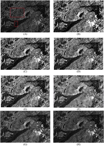
Similar results were obtained for the St. John’s image as depicted in Figure 8. The effect of speckle can be discerned in the original image and as expected, the average filter indiscriminately filtered all parts of the image by the same amount. The MMSE filter maintained the details but isolated points can be clearly noted. A similar outcome can be observed in the enhanced Lee filtered image, but some features were better preserved, such as the urban part near the bottom right of the image. The Gamma filter has also retained the details, but still there are many isolated bright points throughout the image and some parts not being filtered completely. The PPB filter effectively reduced speckle, but some subtle structures remain obscured. The proposed average filter with adaptive window size, on the other hand, filtered the homogeneous areas reasonably well, while it has maintained the details. Isolated points cannot be observed anymore. Even better results have been achieved using the MMSE filter with adaptive window size, where the smaller objects are preserved better.

Figure 8. St. John’s: (A) original one-look HH intensity image. The rectangle on the top and the bottom of the image shows the regions used for computation of coefficient of variation and ENL, respectively, (B) the 5 × 5 average filtered image, (C) the 5 × 5 MMSE (Lee 1980, 1981a) filtered image, (D) the 5 × 5 enhanced Lee (Lopes, Touzi, and Nezry 1990) filtered image, (E) the 5 × 5 Gamma (Lopes et al. 1993) filtered image, (F) PPB (Deledalle, Denis, and Tupin 2009) filtered image with hw = 10, hd = 3, and 4 iterations, (G)average filtered image with adaptive window size, and (H) MMSE filtered image with adaptive window size.

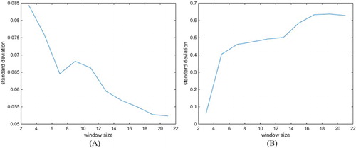
 Figure 9 demonstrates the variation in standard deviation with the change in filtering window size for a pixel located in a homogeneous and a heterogeneous area from the San Francisco image, respectively. The homogeneous region was selected from the ocean on the top right of Figure 7 and the heterogeneous area was chosen from the urban area on the bottom right of Figure 7. Theoretically, as proven in Section 2.1, a large window size is needed in a large, homogeneous area. This is the case in the represented homogeneous region in which the minimum standard deviation corresponds to the largest possible window size. On the other hand, in a heterogeneous area, a small window size suffices. This fact was realized in the representative heterogeneous area in which the minimum standard deviation corresponds to the smallest possible window size. It should be noted that these examples are just two extreme instances amongst many other possible cases.

Figure 9. The variation in standard deviation with the change in the filtering window size. (A) A homogeneous pixel and (B) a heterogeneous pixel.

4.1.3. Assessment of the results

An ideal speckle filter should reduce the amount of speckle in homogeneous regions while preserving the details of the image in heterogeneous areas. Moreover, it should not introduce any bias into the image after filtering. To evaluate the performance of the image from the various mentioned aspects, therefore, computation of some indices is necessary.

For the assessment of the performance of the filter in homogeneous regions, the common measure for estimation of speckle level in the image, namely equivalent number of looks (ENL) was selected. The number of looks is an appropriate measure for estimating the amount of speckle in the image, which is proportional to the speckle standard deviation to mean ratio (Lee and Pottier 2009). For an intensity image, the ENL is defined as (Lee and Pottier 2009):(15) calculated over a large, homogenous area. A high value for ENL shows that speckle was suppressed effectively. It should be noted that the value of ENL, estimated by Equation (15) is usually less than the actual number of looks as a result of spatial correlation (Lee and Pottier 2009).

For the images available for this paper, ENL was calculated over the ocean in the top right of the San Francisco image (Figure 7) and over the large lake in the St. John’s image (Figure 8). The results are shown in Table 2. As can be viewed in Table 2, the value of estimated ENL for both original images is less than but close to 1, as expected. The average filtered images have the highest value of ENL over all filtered images which shows the relatively effective suppression of speckle. The MMSE, enhanced Lee, Gamma, and PPB filters have a lower ENL which indicates the presence of speckle remaining in homogeneous parts of the images. By comparison, the average filter with adaptive window size reduced speckle almost as much as the average filter; and the MMSE filter with adaptive window size has a slightly smaller ENL, while this value is still higher than the corresponding values for the MMSE, enhanced Lee and Gamma filters.

Table 2. Various indices for evaluation and comparison of the performance of the proposed speckle filters on real SAR images.

Image	San Francisco				St. John’s
	ENL				ENL
Original image	0.9233	2.6284	1	1	0.8919	0.8908	1	1
Average filter	11.2384	1.7112	0.9663	0.9564	10.4493	0.7713	0.9653	0.9563
MMSE filter (Lee 1980, 1981a)	7.2548	2.8251	0.9100	0.7612	7.0836	0.9611	0.9086	0.7637
Enhanced Lee filter (Lopes, Touzi, and Nezry 1990)	6.0499	3.7046	0.9360	0.7528	5.7243	1.0963	0.9317	0.7572
Gamma filter (Lopes et al. 1993)	6.8299	4.0011	1.0051	0.8108	5.7897	1.1009	1.0062	0.8079
PPB filter (Deledalle, Denis, and Tupin 2009)	6.9235	2.4647	0.6149	0.5231	5.7930	0.7014	0.7760	1.5383
Average filter with adaptive window size	10.4822	1.003	1.1394	1.5280	10.2089	0.7065	1.1356	1.4085
MMSE filter with adaptive window size	9.3041	2.7543	1.0037	0.9078	9.3788	0.8479	1.0152	0.8793

For estimating the level of texture preservation in heterogeneous areas, a comparison can be made between the coefficient of variation computed over the despeckled image, namely , with its corresponding theoretical value, , as mentioned in Touzi (2002). It can be concluded that loss of radiometric information leads to while injection of impairments can yield (Argenti et al. 2013). and are defined as:(16) (17) where and are the coefficient of variation of the noisy image and speckle noise, respectively, and is the despeckled image (Touzi 2002). for the original image and for all filtered images have been computed over a heterogeneous area in both San Francisco (Figure 7) and St. John’s (Figure 8) images and the results are depicted in Table 2. As can be observed, the average filter poorly preserved the textural information in the images from both areas. MMSE, enhanced Lee, and Gamma filters have larger coefficients of variation in comparison with the original image which suggests that these filters introduced some impairment to the original image. The PPB filter yielded a slightly lower coefficient of variation with respect to the original image, which signifies a slight blurring in texture. Average filter with adaptive window size resulted in a significantly lower coefficient of variation, which implies that this filter performs poorly in maintaining textural patterns. MMSE filter with adaptive window size, however, has the closest coefficient of variation to the original image in both areas, which shows that this filter had the best performance in texture preservation amongst all examined speckle filters.

Another useful measure for evaluating the overall performance of a speckle filter is the ratio image which is defined as:(18) where is the noisy and is the despeckled image (Oliver and Quegan 2004). An ideal speckle filter yields a purely random ratio image while a poor speckle filter causes some patterns to be visible in the image (Argenti et al. 2013). The mean and standard deviation of the ratio image should be as close as possible to the theoretical values of speckle statistics (Argenti et al. 2013). Both of these values are 1 for a single-look image (Solbø and Eltoft 2008).

Ratio images resulting from all filtered images for both the San Francisco and St. John’s areas are illustrated in Figures 10 and 11, respectively. Over both areas, some structures are visible in the enhanced Lee, Gamma, and PPB filters, while the ratio images resulting from the average filter with adaptive window size and the MMSE filter with adaptive window size have an almost random pattern. For a more accurate comparison, however, some numerical indices are necessary.

Figure 10. San Francisco: ratio images resulted from: (A) the 5 × 5 average filtered image, (B) the 5 × 5 MMSE (Lee 1980, 1981a) filtered image, (C) the 5 × 5 enhanced Lee (Lopes, Touzi, and Nezry 1990) filtered image, (D) the 5 × 5 Gamma (Lopes et al. 1993) filtered image, (E) PPB (Deledalle, Denis, and Tupin 2009) filtered image with hw = 20, hd = 5, and 1 iteration, (F) average filtered image with adaptive window size, and (G) MMSE filtered image with adaptive window size from the San Francisco image.

Figure 11. St. John’s: ratio images resulted from: (A) the 5 × 5 average filtered image, (B) the 5 × 5 MMSE (Lee 1980, 1981a) filtered image, (C) the 5 × 5 enhanced Lee (Lopes, Touzi, and Nezry 1990) filtered image, (D) the 5 × 5 Gamma (Lopes et al. 1993) filtered image, (E) PPB (Deledalle, Denis, and Tupin 2009) filtered image with hw = 10, hd = 3, and 4 iterations, (F) average filtered image with adaptive window size, and (G) MMSE filtered image with adaptive window size from the San Francisco image.

The statistics were computed for the ratio image of all filtered images over both areas and the results are illustrated in Table 2. The mean and standard deviation of the ratio image resulted from the average filter is close to 1 which illustrates an unbiased performance. The value of the ratio image’s mean for MMSE, enhanced Lee, and Gamma filters is close to 1. However, standard deviation of the ratio image of these filters differs significantly from the expected theoretical value. This is also true for the mean and standard deviation of the ratio image resulting from the PPB filter. The mean and standard deviation of the ratio image that resulted from the average filter with adaptive window size have a considerable difference with 1, which suggests that the filtering process introduces some bias into the image. The statistics computed from the ratio image of MMSE filter with adaptive window size, however, have almost the closest values to 1, which shows that this filter introduces a small amount of bias to the image after filtering.

Also, for estimating the degree of details preserved visually, a small subset from the urban area of both images is selected to be investigated more closely. These subsets are represented in Figures 12 and 13.

Figure 12. A small subset of the San Francisco image (A) original one-look HH intensity image, (B) the 5 × 5 average filtered image, (C) the 5 × 5 MMSE (Lee 1980, 1981a) filtered image, (D) the 5 × 5 enhanced Lee (Lopes, Touzi, and Nezry 1990) filtered image, (E) the 5 × 5 Gamma (Lopes et al. 1993) filtered image, (F) PPB (Deledalle, Denis, and Tupin 2009) filtered image with hw = 20, hd = 5, and 1 iteration, (G) average filtered image with adaptive window size, and (H) MMSE filtered image with adaptive window size highlighting urban areas from the San Francisco image.

Figure 13. A small subset of St. John’s (A) original one-look HH intensity image, (B) the 5 × 5 average filtered image, (C) the 5 × 5 MMSE (Lee 1980, 1981a) filtered image, (D) the 5 × 5 enhanced Lee (Lopes, Touzi, and Nezry 1990) filtered image, (E) the 5 × 5 Gamma (Lopes et al. 1993) filtered image, (F) PPB (Deledalle, Denis, and Tupin 2009) filtered image with hw = 10, hd = 3, and 4 iterations, (G) average filtered image with adaptive window size, and (H) MMSE filtered image with adaptive window size highlighting urban areas from the St. John’s image.

The original San Francisco small sub-image illustrated in Figure 12 is affected by speckle and the buildings in the urban area seem disconnected. The average filter almost reduced speckle but the small objects are severely blurred. The MMSE filter balanced reducing speckle and retaining the details. However, the boundaries in the built-up area are smeared. If a window size larger than 5 × 5 was used, this effect would be more serious. The enhanced Lee filter blurred the building boundaries in some parts, and disconnected them in other parts. The Gamma filter has filtered the image unevenly and the different parts of the urban area are either blurred or speckled. The PPB filter reduced speckle with slight over-filtering in urban areas. The average filter with adaptive window size successfully maintained the shape of the buildings and reduced speckle, except for some objects which have been overly filtered. Finally, the MMSE filter with adaptive window size has the best performance, preserving the shapes in Figure 12 as well and reducing speckle effectively.

The small sub-image from St. John’s shows similar results. The urban area is severely affected by speckle in the original image in such a way that this part can hardly be discerned visually; the average filter destroyed the details. The urban area can be better distinguished from other parts in the images filtered by MMSE, enhanced Lee, and Gamma filters, but speckle and isolated points are still present. The PPB filter successfully preserved the details, but a few subtle features are lost. Although the average filter with adaptive window size caused slight blurring, it yielded a clear image for the urban area and reduced speckle evenly throughout this region. Finally, the MMSE filter with adaptive window size compensated for the overly filtered parts in the average filtered image with adaptive window size, offering an efficiently speckle-reduced image.

4.2. Polarimetric case

4.2.1. Simulated PolSAR image

In order to test the performance of the proposed method for PolSAR data, two PolSAR images without and with speckle (Figure 14(A,B)) were simulated using the Monte Carlo simulation explained in Lee and Pottier (2009). First, for a covariance matrix, was generated such that:(19) where denotes the conjugate transpose. Then, a complex vector, , is simulated which has a normal distribution with zero mean and an identity covariance matrix. Then, the single-look vector () can be obtained using the following equation:(20)

Figure 14. Simulated PolSAR images: (A) the ground-truth images, (B) the original polarimetric images, (C) the 5 × 5 average filtered images, (D) Images filtered with 5 × 5 refined PolSAR filter (Lee, Grunes, and De Grandi 1999), (E) average filtered images with adaptive window size, and (F) PolSAR filtered images with adaptive window size.

Figure 14 illustrates the result of applying the proposed polarimetric filters to two simulated PolSAR images. For the sake of comparison, the results of applying the average polarimetric filter and the Lee PolSAR filter (Lee, Grunes, and De Grandi 1999) on both images are also shown in Figure 14(C,D), respectively. As can be observed, the average polarimetric filter blurred the boundaries. Moreover, the Lee PolSAR filter failed to completely remove speckle, and left some bright point in the image. The two proposed methods, however, suppressed speckle more effectively, and maintained the boundaries successfully.

4.2.2. Real PolSAR image

The proposed filtering algorithms for multi-polarized images, namely average filtering and polarimetric filtering with adaptive window size, were implemented on both full-polarimetric RADARSAT-2 images. For comparison, typical average filtering and the Lee PolSAR filter (Lee, Grunes, and De Grandi 1999), as well as more advanced methods, namely Lopez (Lopez-Martinez and Fabregas 2008) and Intensity Driven Adaptive Neighbourhood (IDAN) (Vasile et al. 2006) filters, were applied on the image. The results for the San Francisco image are depicted in Figure 15. A Google Earth^TM snapshot for the San Francisco region was included in Figure 15 for a closer visual investigation. 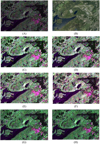The original SAR image is represented in false colour composite, having as the red, as the green and as the blue channel which is clearly affected by speckle. The average filter, although reducing speckle, caused severe blurring in the image. The refined PolSAR filter shows significant improvement, but small details, for example, in the urban area in the bottom right of the image, are smeared. The Lopez filter efficiently filtered the image, but some occasional brighter points are visible in the image and the urban area is slightly blurred. The IDAN filter has effectively reduced speckle while maintaining the details, which shows the value of the adaptive neighbourhood. The average filter with adaptive window size also retained the details, suppressing speckle effectively with minimal over-filtering of some parts, although these parts cannot be easily distinguished. Finally, PolSAR filter with adaptive window size performed very well, by both reducing speckle and preserving the details.

Figure 15. San Francisco: (A) original polarimetric image, (B) snapshot of the study area from Google Earth^TM, (C) the 5 × 5 average filtered image, (D) image filtered with 5 × 5 refined PolSAR filter (Lee, Grunes, and De Grandi 1999), (E) the 5 × 5 Lopez (Lopez-Martinez and Fabregas 2008) filtered image, (F) IDAN (Vasile et al. 2006) filtered image with window size row of 50, (G) average filtering with adaptive window size, and (H) PolSAR filtering with adaptive window size.

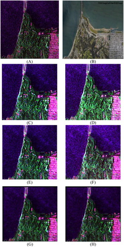
Analogous results were achieved for the St. John’s full-polarimetric image, as represented in Figure 16. Aerial images have also been used for assistance in visual inspection. The polarimetric average filter blurred the details. The refined PolSAR and Lopez filters made a considerable improvement, but the details have been slightly over-filtered, and an amount of speckle is still remaining. A non-speckled, clear image indicates that IDAN filter performed effectively. The polarimetric average filter with adaptive window size offered a smooth part in terms of homogeneous regions, and maintained the details of subtle points. The PolSAR filter with adaptive window size outputted almost the same image, preserving slightly more details in the urban part.

Figure 16. St. John’s: (A) original polarimetric image, (B) snapshot of the study area from Google Earth^TM, (C) the 5 × 5 average filtered image, (D) image filtered with 5 × 5 refined PolSAR filter (Lee, Grunes, and De Grandi 1999), (E) the 5 × 5 Lopez (Lopez-Martinez and Fabregas 2008) filtered image, (F) IDAN (Vasile et al. 2006) filtered image with window size row of 50, (G) average filtering with adaptive window size, and (H) PolSAR filtering with adaptive window size.

5. Discussion

It was observed in previous sections that the proposed adaptive window approach works well with single-band and multi-polarized SAR data. This method also can be applied to partially polarized data, using available real and imaginary channels for estimating the best window size, and then applying the result to the intensity image.

A disadvantage of the proposed method is its computational complexity. In a typical filtering process, the filtering size is manually selected which causes the filter to have a low computational complexity, but at the expense of either losing some detail or leaving speckle in the image. The proposed method looks for the best window size for each pixel, and then applies the filter on it. For improving the computational complexity of the method, narrowing the range of window sizes for filtering each pixel based on a heterogeneity measure is suggested to improve the computational complexity of the method in future studies.

Some practical considerations are necessary when implementing the proposed algorithm. In the range of window sizes which are selected for filtering the real and imaginary images, the minimum window size is more important than the maximum one. If the minimum window size is too large, some details in the image might be blurred. Thus, care must be taken in selecting the minimal window size; the most conservative choice for that is 3 × 3.

Computing the optimal window size using both real and imaginary images helps to estimate the best window size more accurately, but using one of them suffices. This is also true for the polarimetric filter, where all real and imaginary images are used for estimating the most appropriate filtering size. Although the three channels have different features, the definition of object is the same in all of them, although they might appear diversely in each band. Accordingly, optimal window size for each pixel must be the same for all channels.

6. Conclusion

Using a single fixed-size rectangular window is not effective for speckle filtering of SAR images, owing to the fact that objects with different sizes need different filtering windows. To address this issue, the paper presents a novel technique for filtering with adaptive window size. The method applies windows with changing sizes throughout the image based on local information (i.e. standard deviation) computed from neighbouring pixels. To find an optimal window size for each pixel, windows with various sizes are applied to real and imaginary SAR images separately, and the window with minimum standard deviation is chosen as the optimum window size for filtering. It was demonstrated that the window which yields the minimal standard deviation for each pixel over the whole range of sizes has the optimal size for filtering that pixel. The method was applied to single-look intensity data, but it can be applied to multi-look and amplitude images as well. The filter has been proposed in single-band and polarimetric versions, and average and MMSE filtering methods with adaptive window size have been provided in both cases. The proposed methods outperform their fixed-size counterparts both in single-band and in polarimetric versions. This approach can preserve the details of the image while suppressing speckle effectively. The computational complexity of the proposed filters is greater than their fixed-size counterparts because the suggested algorithms look for the appropriate window size for each pixel, while in the typical filters the window size is fixed. The computational complexity, however, may be reduced. Finally, adjusting other filters so that they may be applied with adaptive window size is a valuable area of future study.

Disclosure statement

No potential conflict of interest was reported by the authors.

Additional information

Funding

This project was undertaken with the financial support of the Government of Canada through the federal Department of Environment and Climate Change, and the Research & Development Corporation of Newfoundland and Labrador. The SAR imagery was provided by the Canada Center for Mapping and Earth Observation and Environment and Climate Change Canada. The authors thank these organizations for the generous financial supports and providing such valuable datasets.

References

- Argenti, Fabrizio, Alessandro Lapini, Tiziano Bianchi, and Luciano Alparone. 2013. “A Tutorial on Speckle Reduction in Synthetic Aperture Radar Images.” IEEE Geoscience and Remote Sensing Magazine 1 (3): 6–35. doi: 10.1109/MGRS.2013.2277512
- Boerner, W. M., H. Mott, E. Lüneburg, C. Livingstone, B. Brisco, R. J. Brown, and J. S. Paterson. 1998. “Polarimetry in Radar Remote Sensing: Basic and Applied Concepts.” In Principles and Applications of Imaging Radar, Manual of Remote Sensing, edited by A. J. Lewis and F. M. Henderson, 271–358. New York: Wiley.
- Chen, Jiong, Yilun Chen, Wentao An, Yi Cui, and Jian Yang. 2011. “Nonlocal Filtering for Polarimetric SAR Data: A Pretest Approach.” IEEE Transactions on Geoscience and Remote Sensing 49 (5): 1744–1754. doi: 10.1109/TGRS.2010.2087763
- Datcu, Mihai, Klaus Seidel, and Marc Walessa. 1998. “Spatial Information Retrieval from Remote-Sensing Images. I. Information Theoretical Perspective.” IEEE Transactions on Geoscience and Remote Sensing 36 (5): 1431–1445. doi: 10.1109/36.718847
- Deledalle, Charles-Alban, Loïc Denis, and Florence Tupin. 2009. “Iterative Weighted Maximum Likelihood Denoising with Probabilistic Patch-based Weights.” IEEE Transactions on Image Processing 18 (12): 2661–2672. doi: 10.1109/TIP.2009.2029593
- Deledalle, Charles-Alban, Loïc Denis, and Florence Tupin. 2011. “NL-InSAR: Nonlocal Interferogram Estimation.” IEEE Transactions on Geoscience and Remote Sensing 49 (4): 1441–1452. doi: 10.1109/TGRS.2010.2076376
- Deledalle, Charles-Alban, Florence Tupin, and Loïc Denis. 2010. “ A Non-local Approach for SAR and Interferometric SAR Denoising.” Paper Presented at the IEEE International Geoscience and Remote Sensing Symposium (IGARSS).
- Durand, Jean M., Bernard J. Gimonet, and Jacqueline R. Perbos. 1987. “SAR Data Filtering for Classification.” IEEE Transactions on Geoscience and Remote Sensing 5: 629–637. doi: 10.1109/TGRS.1987.289842
- Frost, V. S., J. A. Stiles, K. Sam Shanmugam, J. C. Holtzman, and S. A. Smith. 1981. “An Adaptive Filter for Smoothing Noisy Radar Images.” Paper Presented at the IEEE Proceedings.
- Frost, Victor S., Josephine Abbott Stiles, K. Sam Shanmugan, and Julian C. Holtzman. 1982. “A Model for Radar Images and its Application to Adaptive Digital Filtering of Multiplicative Noise.” IEEE Transactions on Pattern Analysis and Machine Intelligence 2: 157–166. doi: 10.1109/TPAMI.1982.4767223
- Goze, S., and A. Lopes. 1993. “A MMSE Speckle Filter for Full Resolution SAR Polarimetric Data.” Journal of Electromagnetic Waves and Applications 7 (5): 717–737. doi: 10.1163/156939393X00831
- Korostelev, Aleksandr Petrovich, and Olga Korosteleva. 2011. Mathematical Statistics: Asymptotic Minimax Theory, Vol. 119. Providence, RI: American Mathematical Soc.
- Kuan, Darwin T., Alexander Sawchuk, Timothy C. Strand, and Pierre Chavel. 1985. “Adaptive Noise Smoothing Filter for Images with Signal-dependent Noise.” IEEE Transactions on Pattern Analysis and Machine Intelligence 2: 165–177. doi: 10.1109/TPAMI.1985.4767641
- Kuan, Darwin T., Alexander Sawchuk, Timothy C. Strand, and Pierre Chavel. 1987. “Adaptive Restoration of Images with Speckle.” IEEE Transactions on Acoustics, Speech, and Signal Processing 35 (3): 373–383. doi: 10.1109/TASSP.1987.1165131
- Lang, Fengkai, Jie Yang, and Deren Li. 2015. “Adaptive-Window Polarimetric SAR Image Speckle Filtering Based on a Homogeneity Measurement.” IEEE Transactions on Geoscience and Remote Sensing 53 (10): 5435–5446. doi: 10.1109/TGRS.2015.2422737
- Lee, Jong-Sen. 1980. “Digital Image Enhancement and Noise Filtering by use of Local Statistics.” IEEE Transactions on Pattern Analysis and Machine Intelligence 2: 165–168. doi: 10.1109/TPAMI.1980.4766994
- Lee, Jong-Sen. 1981a. “Refined Filtering of Image Noise Using Local Statistics.” Computer Graphics and Image Processing 15 (4): 380–389. doi: 10.1016/S0146-664X(81)80018-4
- Lee, Jong-Sen. 1981b. “Speckle Analysis and Smoothing of Synthetic Aperture Radar Images.” Computer Graphics and Image Processing 17 (1): 24–32. doi: 10.1016/S0146-664X(81)80005-6
- Lee, Jong-Sen. 1983a. “Digital Image Smoothing and the Sigma Filter.” Computer Graphics and Image Processing 24 (2): 255–269. doi: 10.1016/0734-189X(83)90047-6
- Lee, Jong-Sen. 1983b. “A Simple Speckle Smoothing Algorithm for Synthetic Aperture Radar Images.” IEEE Transactions on Systems, Man, and Cybernetics 1: 85–89. doi: 10.1109/TSMC.1983.6313036
- Lee, Jong-Sen. 1986. “Speckle Suppression and Analysis for Synthetic Aperture Radar Images.” Optical Engineering 25 (5): 255636. doi: 10.1117/12.7973877
- Lee, Jong-Sen, Thomas L. Ainsworth, Yanting Wang, and Kun-Shan Chen. 2015. “Polarimetric SAR Speckle Filtering and the Extended Sigma Filter.” IEEE Transaction Geoscience and Remote Sensing 53 (3): 1150–1160. doi: 10.1109/TGRS.2014.2335114
- Lee, Jong-Sen, Shane R. Cloude, Konstantinos P. Papathanassiou, Mitchell R Grunes, and Iain H Woodhouse. 2003. “Speckle Filtering and Coherence Estimation of Polarimetric SAR Interferometry Data for Forest Applications.” IEEE Transactions on Geoscience and Remote Sensing 41 (10): 2254–2263. doi: 10.1109/TGRS.2003.817196
- Lee, Jong-Sen, Mitchell R. Grunes, and Gianfranco De Grandi. 1999. “Polarimetric SAR Speckle Filtering and its Implication for Classification.” IEEE Transactions on Geoscience and Remote Sensing 37 (5): 2363–2373. doi: 10.1109/36.789635
- Lee, Jong-Sen, Mitchell R. Grunes, and Stephen Mango. 1991. “Speckle Reduction in Multipolarization, Multifrequency SAR Imagery.” IEEE Transaction Geoscience and Remote Sensing 29 (4): 535–544. doi: 10.1109/36.135815
- Lee, Jong-Sen, Mitchell R. Grunes, Dale L. Schuler, Eric Pottier, and Laurent Ferro-Famil. 2006. “Scattering-model-based Speckle Filtering of Polarimetric SAR Data.” IEEE Transactions on Geoscience and Remote Sensing 44 (1): 176–187. doi: 10.1109/TGRS.2005.859338
- Lee, Jong-Sen, L. Jurkevich, P. Dewaele, P. Wambacq, and A. Oosterlinck. 1994. “Speckle Filtering of Synthetic Aperture Radar Images: A Review.” Remote Sensing Reviews 8 (4): 313–340. doi: 10.1080/02757259409532206
- Lee, Jong-Sen, and Eric Pottier. 2009. Polarimetric Radar Imaging: From Basics to Applications. New York: CRC Press.
- Lee, Jong-Sen, Jen-Hung Wen, Thomas L. Ainsworth, Kun-Shan Chen, and Alex Jianzhong Chen. 2009. “Improved Sigma Filter for Speckle Filtering of SAR Imagery.” IEEE Transactions on Geoscience and Remote Sensing 47 (1): 202–213. doi: 10.1109/TGRS.2008.2001637
- Lopes, A., E. Nezry, R. Touzi, and H. Laur. 1993. “Structure Detection and Statistical Adaptive Speckle Filtering in SAR Images.” International Journal of Remote Sensing 14 (9): 1735–1758. doi: 10.1080/01431169308953999
- Lopes, Armand, and Franck Séry. 1997. “Optimal Speckle Reduction for the Product Model in Multilook Polarimetric SAR Imagery and the Wishart Distribution.” IEEE Transactions on Geoscience and Remote Sensing 35 (3): 632–647. doi: 10.1109/36.581979
- Lopes, Armand, Ridha Touzi, and E. Nezry. 1990. “Adaptive Speckle Filters and Scene Heterogeneity.” IEEE Transactions on Geoscience and Remote Sensing 28 (6): 992–1000. doi: 10.1109/36.62623
- Lopez-Martinez, Carlos, and Xavier Fabregas. 2008. “Model-based Polarimetric SAR Speckle Filter.” IEEE Transactions on Geoscience and Remote Sensing 46 (11): 3894–3907. doi: 10.1109/TGRS.2008.2002029
- Nicolas, J.-M., F. Tupin, and H. Maître. 2001. “Smoothing Speckled SAR Images by Using maximum Homogeneous Region Filters: An Improved Approach.” Paper presented at the IEEE International Geoscience and Remote Sensing Symposium, IGARSS'01.
- Novak, Leslie M., and Michael C. Burl. 1990. “Optimal Speckle Reduction in Polarimetric SAR Imagery.” IEEE Transactions on Aerospace and Electronic Systems 26 (2): 293–305. doi: 10.1109/7.53442
- Oliver, Chris, and Shaun Quegan. 2004. Understanding Synthetic Aperture Radar Images. Raleigh, NC: SciTech Publishing.
- Park, J.-M., Woo-Jin Song, and W. A. Pearlman. 1999. “Speckle Filtering of SAR Images Based on Adaptive Windowing.” Paper presented at the Vision, Image and Signal Processing, IEE proceedings.
- Solbø, Stian, and Torbjørn Eltoft. 2008. “A Stationary Wavelet-Domain Wiener Filter for Correlated Speckle.” IEEE Transactions on Geoscience and Remote Sensing 46 (4): 1219–1230. doi: 10.1109/TGRS.2007.912718
- Therrien, Charles, and Murali Tummala. 2011. Probability and Random Processes for Electrical and Computer Engineers. Boca Raton, FL: CRC Press.
- Torres, Leonardo, Sidnei J. S Sant'Anna, Corina da Costa Freitas, and Alejandro C. Frery. 2014. “Speckle Reduction in Polarimetric SAR Imagery with Stochastic Distances and Nonlocal Means.” Pattern Recognition 47 (1): 141–157. doi: 10.1016/j.patcog.2013.04.001
- Touzi, Ridha. 2002. “A Review of Speckle Filtering in the Context of Estimation Theory.” IEEE Transactions on Geoscience and Remote Sensing 40 (11): 2392–2404. doi: 10.1109/TGRS.2002.803727
- Vasile, Gabriel, Emmanuel Trouvé, J. Lee, and Vasile Buzuloiu. 2006. “Intensity-driven Adaptive-Neighborhood Technique for Polarimetric and Interferometric SAR Parameters Estimation.” IEEE Transactions on Geoscience and Remote Sensing 44 (6): 1609–1621. doi: 10.1109/TGRS.2005.864142
- Walessa, Marc, and Mihai Datcu. 2000. “Model-based Despeckling and Information Extraction from SAR Images.” IEEE Transactions on Geoscience and Remote Sensing 38 (5): 2258–2269. doi: 10.1109/36.868883
- Wang, Zhou, Alan Conrad Bovik, Hamid Rahim Sheikh, and Eero P. Simoncelli. 2004. “Image Quality Assessment: From Error Visibility to Structural Similarity.” IEEE Transactions on Image Processing 13 (4): 600–612. doi: 10.1109/TIP.2003.819861