A new method for generating a clear-sky Landsat composite for cropland from cloud-contaminated Landsat-7 and Landsat-8 images

ABSTRACT

A new method was developed in this study for producing a clear-sky Landsat composite for cropland from cloud-contaminated Landsat images acquired in a short time period. It used Thiel–Sen regression to normalize all Landsat scenes to a MODIS image to make all Landsat images radiometrically consistent and comparable. Pixel selection criteria combining the modified maximum vegetation index and the modified minimum visible reflectance selection methods were designed to enhance the pixel selection of land/water over cloud/shadow in the image compositing. The advantages of the method include (1) avoiding complicated atmospheric corrections but with reliable surface reflectance results, (2) being insensitive to errors induced by image co-registration uncertainties between Landsat and MODIS images, (3) avoiding the lack of samples for the regression analysis using the full Landsat scenes (rather than overlay regions), and (4) enhancing cloud/shadow detection. The composite image has MODIS-like surface reflectance, thus making MODIS algorithms applicable for retrieving biophysical parameters. The method was automatically implemented on a set of 13 cloud-contaminated (>39%) Landsat-7 (Scan-Line Corrector-Off) and Landsat-8 scenes acquired during peak growing season in a crop region of Manitoba, Canada. The result was a 95.8% cloud-free image. The method can also substantially increase the usage of cloud-contaminated Landsat data.

KEYWORDS:

• Landsat
• compositing
• MODIS
• Thiel–Sen regression

1. Introduction

Landsat imagery is widely used for mapping and monitoring large-scale environmental changes due to its over 40-years data collection, providing global, multi-temporal, and multi-spectral imagery with medium resolutions (10–100 m). Since Landsat-5 was officially decommissioned on 5 June 2013, Landsat-7 (launched in 1999) and Landsat-8 (launched in 2013) have continued to supply images for users. The ETM+ and OLI sensors on board the Landsat-7 and Landsat-8 satellites provide a spatial coverage of 185 × 185 km² per scene with a spatial resolution of 30 m. The relatively long revisit interval of 16 days for these sensors and frequent contamination by cloud largely constrain the data usability for environmental monitoring in a timely manner (Gao et al. 2006). Moreover, a mechanical fault in the Scan-Line Corrector (SLC-Off) of the Landsat-7 satellite has caused missing data strips (22–25% data loss) throughout the images since 2003, further reducing the data usability.

Clouds and the associated cloud shadows often contaminate Landsat imagery acquired for many parts of the world, particularly in humid regions with high evapotranspiration (Hughes and Hayes 2014; Martinuzzi, Gould, and Ramos Gonzalez 2006; Wang 2008; Wang et al. 2013). For example, Zhou and Zhang (2013) reported that there were at least 10 cloudy days in a month for every location in southern Canada. The chance of obtaining a cloud-free Landsat image (cloud cover < 10%) during the peak growing season of July and August for some regions in Canada can be as low as 10% (Leckie 1990). The cloud and cloud shadow contamination is a particular concern in applying Landsat data for monitoring land surface with more dynamic change such as agricultural ecosystems, which may have inter-annual changes in crop types due to crop rotation or different phenological stages in a short time window. It is often difficult to get a cloud-free Landsat image for the specific season or year of interest required in crop mapping. As such, an essential task for applying optical satellite imagery is to generate cloud-free or clear-sky image composites from multiple images covering the same area (Cihlar 1996).

Various compositing methods have been developed for sensors with low spatial resolutions such as AVHRR, MODIS, VEGETATION, and MERIS (Cihlar and Howarth 1994; Luo, Trishchenko, and Khlopenkov 2008; Simpson and Stitt 1998). Generally, these methods include (1) cloud and cloud shadow identification for producing a cloud/shadow mask for each individual scene, (2) producing a clear-sky composite image at Top of Atmospheric (TOA) for a specific period, (3) atmospheric correction using a physical radiative transfer model for obtaining a clear-sky composite image at the surface, and (4) BRDF (Bidirectional Reflectance Distribution Function) correction for normalizing angular surface reflectance to a common viewing geometry (e.g. nadir-view). However, image compositing was not often considered for medium-resolution data until recently due to high data cost.

NASA and US Geological Survey (USGS) have recently implemented a new data policy that provides free access to Landsat data. Landsat-based compositing approaches have been developed to produce large area composites for large-area applications (Griffiths et al. 2013; Potapov, Turubanova, and Hansen 2011). For example, Landsat image composites for large areas have been produced to map aboveground biomass over the west arctic region of Canada, and to map boreal forest changes in Russia (Chen et al. 2009; Potapov, Turubanova, and Hansen 2011). The composited Landsat/ETM+ top-of-atmosphere imagery covering the USA has been made available via a web interface (Roy et al. 2010). Recently, researchers have made effort to develop methods that compose cloud-free Landsat image from multi-temporal images with the aid of cloud-free images/patches (Han, Francesca, and Lee 2017; Lin et al. 2013, 2014; Xu et al. 2016). However, these methods either rely on cloud-free reference images/patches or overlay regression models for radiometric normalization, selecting ‘best pixel’ based on a single spectral criterion, or they do not use surface reflectance (Griffiths et al. 2013). Therefore they may have problems in finding cloud-free reference images, dealing with uncertainties of co-registration among images in radiometric normalization, cloud/shadow residuals or finding enough samples for building normalization models, which may limit their performances. In addition, few Landsat-based compositing algorithms are suitable for regions (e.g. prairie agriculture regions in Canada) with low-acquisition frequency, high cloud cover, and short vegetation growing season (Potapov, Turubanova, and Hansen 2011).

The objective of this study is to get a clear-sky Landsat image for the specific season of interest required in crop applications for prairie agriculture regions in Canada. As such, a new method was proposed to overcome the aforementioned drawbacks in existing compositing methods. The method employs a relative atmospheric correction algorithm by using a MODIS surface reflectance composite as a reference for the radiometric normalization of all the Landsat scenes. It avoids the tedious work associated with atmospheric corrections for a large number of Landsat scenes. The compositing scheme is land-cover dependent and makes use of multi-criteria in selecting clear-sky pixels, which includes the modified maximum VI (vegetation index) and the modified minimum visible reflectance. The goal of this study is to develop an efficient Landsat compositing method by maximizing the usage of all available Landsat images so that the composite can be produced in a period as short as possible.

2. Study area and datasets

The study area covers the Spiritwood valley (Figure 1) with an area of 75 × 75 km². It stretches from southwest Manitoba, Canada to North Dakota, USA. The dominant land cover is agriculture, intermingled with grassland and forests. Surface water is fairly abundant in numerous small waterbodies in this prairie landscape (Li and Wang 2015).

Figure 1. The location of the test site.

All available Landsat-7/ETM+ and Landsat-8/OLI level L1G orthorectified TOA data acquired between 15 July and 11 August 2013 were downloaded from Earth Resources Observation and Science (EROS) Center of USGS. These images either fully or partially cover the study area. There are a total of 13 scenes of which the details are given in Table 1. Among these scenes, the cloud-contaminated and no-data areas (Landsat-7 SLC-off strips or areas not covered by Landsat scene) within our study region range from ∼39% to ∼99%.

Table 1. The list of Landsat scenes.

Satellite/sensor	Path/row	Acquisition date	Cloud/shadow/no-data coverage in the study area (%)
Landsat-7/ETM+	33/25	16 July 2013	99.2
Landsat-7/ETM+	33/26	16 July 2013	99.1
Landsat-7/ETM+	31/26	18 July 2013	99.2
Landsat-7/ETM+	32/26	25 July 2013	69.4
Landsat-7/ETM+	33/25	1 August 2013	96.4
Landsat-7/ETM+	33/26	1 August 2013	87.7
Ladnsat-7/ETM+	31/26	3 August 2013	81.8
Landsat-8/OLI	32/26	17 July 2013	38.7
Landsat-8/OLI	33/25	24 July 2013	86.4
Landsat-8/OLI	33/26	24 July 2013	81.8
Landsat-8/OLI	31/26	26 July 2013	82.1
Landsat-8/OLI	32/26	2 August 2013	44.4
Landsat-8/OLI	31/26	11 August 2013	66.9

The 16-day composite MCD43A4 product is also used in this study, which provides 500 m BRDF-corrected surface reflectance data. To match the acquisition dates of the Landsat images, we downloaded the MCD43A4 composite covering the time period of 20 July–4 August 2013, in tiles h11v03 and h11v04. The MODIS data were mosaicked to cover the study area. The associated MODIS state file was used to filter out pixels contaminated by clouds and cloud shadows so that only high-quality clear-sky surface reflectance data were used for further analysis.

3. Method

The new method includes three major steps: (1) identify clouds and cloud shadows in Landsat-7/Landsat-8 images as well as SLC-off strips in Landsat-7/ETM+ images, (2) normalize all Landsat images to the MODIS surface reflectance image to ensure radiometric consistency, and (3) composite the radiometrically normalized Landsat images. The details for these steps are given below.

3.1. Cloud and cloud shadow identification in Landsat spectral images

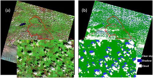
Cloud and cloud shadow identification is an important step towards successful generation of clear-sky composite images. In this study, the Fmask (Function of mask) algorithm recently proposed by Zhu and Woodcock (2012) was used for cloud and cloud shadow detection in Landsat imagery. Fmask is an object-based approach which can produce an accurate cloud and cloud shadow mask. The input data for the algorithm are Landsat TOA reflectance and brightness temperature (BT). For Landsat L1T images, digital number (DN) values are first converted to TOA reflectance and BT (in Celsius degree). Criteria based on water, cloud, and cloud shadow physical properties are then applied to TOA reflectance and BT to extract the potential masks for water, clouds, and cloud shadows. The segmented cloud layer and the geometric relationships of clouds and cloud shadows are used to match the potential cloud shadow layer. More details on the Fmask algorithm can be found in Zhu and Woodcock (2012). An example of a cloud and cloud shadow mask produced for Landsat scene (32/26) is shown in Figure 2. Figure 2(a) shows the Landsat-8 scene composite (red: band 5, green: band 4, blue: band 3), where clouds and the cloud shadows can be visually identified. Figure 2(b) displays the classified map from the Fmask algorithm. Visual examination reveals that the Fmask algorithm performed well in cloud and cloud shadow detection. For Landsat-7 imagery, the SLC-Off strips are also identified in this step.

Figure 2. An example of cloud and cloud shadow detection for the Landsat scene (32/26) acquired on 26 July 2013: (a) the Landsat-8 scene composite (red: SWIR band, green: NIR band, blue: RED band), where clouds and the shadows can be visually identified; (b) classified map derived from the Fmask algorithm.

3.2. Radiometric normalization of Landsat scenes

The objective of radiometric normalization of the Landsat scenes is to make image radiometric signals consistent so that they are comparable among images from different sensors and different acquisition times. Since surface reflectance is a physical measure of surface properties not affected by atmospheric effects and sensor calibration issues, it can be used as the basis for compositing images from different sensors and different acquisition times (Gao et al. 2010). However, due to intrinsic differences in sensor bandwidths or view-illumination geometrics, surface reflectance from different sensors may not be comparable even if satellite data are atmospherically corrected by either a physical radiative transfer model or an empirical approach (Gao et al. 2010). Since the launch of the first Landsat sensor in 1972, numerous relative radiometric normalization approaches have been proposed. These approaches are mostly based on adjusting the radiometric properties of the scenes in the composite to match that of a single reference scene chosen (usually the least contaminated scene) (Olthof et al. 2005). The normalization is often done using the overlap regression methods, including simple regression and more complex outlier resistant approaches (Du, Cihlar, and Latifovic 2001; Olthof et al. 2005). The overlay regression method uses data in overlap regions to generate a function relating radiances of identical features in different images. However, this method is often constrained by the lack of enough suitable invariant features in overlay regions due to cloud, cloud shadow or Landsat-7’s SLC-off. It also brings radiometric error propagation because overlay regions poorly represent whole Landsat scenes (Olthof et al. 2005). To address these weaknesses, we extended this technique by using a simultaneously acquired MODIS surface reflectance image as the reference in this paper. The reason for choosing MODIS surface reflectance as a reference is that MODIS images have similar viewing and solar geometries as Landsat images. Another advantage of our approach is that it enables the use of full Landsat scenes in generating the regression function model.

Differences in spectral bandwidths and spectral response functions of Landsat-7/8 and MODIS may lead to non-linear relationships between their surface reflectance. In this study, we used linear transformations of the response functions between two sensors based on previous studies (e.g. Gao et al. 2010; Teillet et al. 2001). Gao et al. (2010) reported that the differences of surface reflectance between MODIS and Landsat ETM+ with a linear regression normalization (MODIS as reference) were smaller than the theoretical accuracy of MODIS surface reflectance itself. Therefore, a linear regression model is suitable for approximating the non-linear relationships between different sensors. In our normalization approach, the cluster-based pure homogeneous pixels were used as samples for building the regression model, which can deal with various seasonal changes from different surface types (Gao et al. 2010). Instead of using a traditional linear regression model, our normalization approach used the Thiel–Sen regression model. The Thiel–Sen regression fits a line y = mx + b by choosing m to be the median among the n(n−1)/2 slopes of lines determined by the n pairs of data points. The parameter b is found by choosing the median among the values y − mx. The Thiel–Sen regression is a non-parametric robust estimator, which is insensitive to up to 29% of the outliers, thus reducing the effect of data scatter due to atmospheric effects or land cover change (Olthof et al. 2005).

In this relative normalization approach, the K-means clustering algorithm is first applied to Landsat scenes to obtain clustering maps with K clusters. The K-means algorithm provides fast execution and does not require a training stage to produce cluster centers (Li and Chen 2007). After the clustering maps are obtained, the Landsat TOA data are resampled to 500 m resolution to match the resolution of the reference MODIS surface reflectance image by approximating MODIS point spread function (PSF). Due to the effect of PSF, the sensor detectors will expand the actual observation area half a pixel in both along-scan and along-track directions (Tan et al. 2006). It means that the sensor collects signals not only from within that pixel, but also from surrounding pixels (Huang et al. 2002). The MODIS PSF can be represented by a triangular PSF (Tan et al. 2006). To build the Thiel–Sen regression model, we aggregated the Landsat TOA data to 500 m resolution by a resampling process with MODIS PSF applied. The resampling process includes: (1) determining the center pixel of a resampling area (1000 m by 1000 m) in a Landsat image, which corresponds to the center of a MODIS pixel; (2) finding the boundary of the resampling area in the Landsat image; (3) applying weights, which are generated from MODIS PSF, to Landsat pixels within the resampling area to get a pixel average value at 500 m resolution. During resampling, the percentage of the majority cluster within the resampling area is also calculated to represent the homogeneity of the MODIS pixel. Normalization models are then built by conducting the Thiel–Sen regressions between resampled Landsat TOA data and MODIS surface reflectance data by using homogenous MODIS pixels (homogenerity higher than 95%) only. Note that only cloud-free pixels on both Landsat and MODIS images are used for the regression analysis. The state file associated with the MCD43A4 product is used to mask out clouds and cloud shadows in the MODIS image. Different normalization models can be built at cluster level within a scene for individual spectral bands of different Landsat images. Since there may not be enough homogenous samples to build a normalization model for each cluster due to cloud cover or Landsat-7’s SLC-off, Landsat scene-wise normalization models, which use all sampled paring pixels of Landsat and MODIS, were generated separately for individual spectral bands. In the Thiel–Sen regression, the Landsat pixel values are the independent variable and the MODIS pixel values are the response variable. The normalization models are then applied to the original Landsat data to generate MODIS-like surface reflectance data at a 30 m resolution.

3.3. Clear-sky Landsat image compositing

This step is to produce a single clear-sky image by selecting the best pixels among candidates from the single scenes over a pre-defined period of time. Several compositing methods have been applied in previous studies, which include (1) the maximum VI (normalized difference vegetation index (NDVI) or simple ratio of near-infrared (NIR) and red) approach, which is effective for generating composite data for vegetation studies, but has limitations in differentiating cloudy pixels from clear-sky water, water/land mixture or snow/ice pixels, and (2) the minimum visible (VIS) reflectance approach, which is, on the other hand, good at excluding clouds and haze but limited by choosing cloud shadow over clear-sky pixels (Luo, Trishchenko, and Khlopenkov 2008). The available compositing methods mostly rely on a single criterion and are for low-resolution sensors. As found in Luo, Trishchenko, and Khlopenkov (2008), a single universal criterion for all surface conditions is unlikely adequate. Although the Fmask algorithm used in this paper performs well in cloud and cloud shadow detection for Landsat images, the residual clouds (especially haze) and cloud shadows may still exist. In addition, all the Landsat data has been converted to MODIS-like reflectance data after the radiometric normalization process. Therefore, we used a multi-criteria approach, which was proposed by Luo, Trishchenko, and Khlopenkov (2008) for MODIS image composition, for the clear-sky Landsat image compositing. The approach relies on the cloud–shadow–water–land state mask derived for each pixel as described in the previous section. The criteria involve four Landsat bands: blue (b1), red (b3), NIR (b4), and shortwave infrared (SWIR) I (b5). Table 2 shows the application of the compositing criteria on classified pixel pairs.

Table 2. Application of the compositing criteria^a on classified pixel pairs (selected and candidate pixels).

	Land	Water	Cloud	Shadow	Snow/ice
Land	C1	C2	C2	C1s	C2
Water		C2	C2	C2s	C2
Cloud			C2	C2s	C3
Shadow				C1s	C3s
Snow/ice					C3

^aC1: maximum [max(b4, b5)/(b1 + b3)], C1s: maximum [max(b4, b5)/b1], C2: minimum [b1 + b3], and C2s: minimum [b1], C3: maximum [(b3/b5)•(b3 − b5)], and C3s: maximum [(b3/b5)•(b4/b1)² where index ‘s’ marks pixels involving shadows.

Criterion C1 is used when both pixels are identified as clear-sky land. This criterion is an improvement of the maximum simple ratio of NIR and red (b4/b3) criterion, which is equivalent to the maximum NDVI criterion. Since b4 is sensitive to green vegetation and b5 is effective for detecting snow and non-vegetated land, the use of max (b4, b5) ensures that C1 is effective for most land types, whether they are vegetated or non-vegetated. The b3 is often used to separate bright targets (e.g. snow, desert, and cloud) from vegetation and water bodies. The addition of b1 allows C1 to be more effective in removing residual cloud and haze contaminations since b1 is more sensitive to thin cloud and haze than b3. Considering b1 is less sensitive to cloud shadows than b3, we apply C1s (a modification of C1) when a candidate pixel is classified as cloud shadow and another as land. Criterion C2 is applied when at least one candidate is identified as water or cloud. The addition of b1 helps correct misclassification of thin clouds over water as land. Criterion C2s is used for screening cloud shadows over water pixels. Criterion C3 is designed for both pixels being snow or one snow and one cloud. Generally, the reflectance b5 is significantly smaller for snow/ice scenes than for ice clouds. The ratio b3/b5 in C3 is used to enhance the selection of snow because it is usually larger for the real snow/ice scenes than that for ice clouds (Luo, Trishchenko, and Khlopenkov 2008). C3s is used to select snow/ice over cloud shadows. The experiments of Luo, Trishchenko, and Khlopenkov (2008) indicated that the multi-criteria approach substantially improved the quality of composites compared to the maximum VI and the minimum visible reflectance approaches.

4. Results and discussions

The proposed Landsat compositing method was applied to the 7 Landsat-7 scenes acquired between 16 July and 3 August 2014, the 6 Landsat-8 scenes acquired between 17 July and 11 August 2014, and all 13 Landsat-7 and Landsat-8 scenes, separately. Although the first three Landsat-7 images (listed in Table 1) have a small amount (less than 1%) of cloud-free Landsat pixels for the study area, there are enough cloud-free pixels in the whole Landsat images to build normalization models. Once normalized, these small amounts of pixels may be the ‘best’ candidates for the image compositing according to the pixel composite criteria used in this study. Therefore, we kept these images in this study. Three Landsat composite images covering the study area were thus generated. These images are denoted as COM-7 for using Landsat-7 images only, COM-8 for using Landsat-8 images only, and COM-78 for using all Landsat-7 and Landsat-8 images. As stated in Section 3.2, the resultant images have been corrected to surface reflectance during the compositing process. Figure 3(a–c) shows the color-composited surface reflectance map from SWIR I band (as red channel), NIR band (as green channel), and RED band (as blue channel) of the COM-7, COM-8, and COM-78, respectively. As shown in Figure 3(c), a few small areas are still covered by cloud even though all the data was used. This is due to the fact that these areas at all acquisition dates were covered by clouds. The cloud coverages in the final COM-7, COM-8, and COM-78 images are 40.6% and 9.5%, and 4.2%, respectively.

Figure 3. Color-composited surface reflectance maps (SWIR: red channel, NIR: green channel, RED: blue channel) from (a) the composite image produced by using Landsat-7 imagery only (b) the composite image produced by using Landsat-8 only and (c) the composite image produced by using both Landsat-7 and Landsat-8 imagery.

In the radiometric normalization, a high homogeneity threshold (>95%) of MODIS pixels was used for building the regression models. Figure 4 shows an example of the Thiel–Sen regression models between Landsat TOA reflectance (scene 32/26 acquired on 26 July 2013) and MODIS surface reflectance for red band (Figure 4(a)), NIR band (Figure 4(b)), and SWIR I band (Figure 4(c)), respectively. Good linear relations for all three bands are achieved. It must be emphasized that the Landsat TOA reflectance is directly converted to surface reflectance when it is normalized to the MODIS surface reflectance. The radiometric normalization process in the new method avoided the tedious work associated with atmospheric corrections for a large number of Landsat scenes. The differences of surface reflectance derived by the radiometric normalization approach and the atmospheric correction approach based on radiative transfer models have been reported as very small to within ±0.02 of true reflectance (Chen, Chen, and Li 2010; Gao et al. 2010). As such, the radiometric normalization can be used as an alternative approach for fast and reliable retrieval of surface reflectance from Landsat data. However, due to the bandwidth differences between Landsat and MODIS, it must be noted that our corrected surface reflectance is a MODIS-like data.

Figure 4. Thiel–Sen regression models between Landsat TOA reflectance (scene 32/26 acquired on 26 July 2013) and MODIS surface reflectance for (a) RED band, (b) NIR band, and (c) SWIR band.

To validate the spectral fidelity of the COM-78 image, a clear-sky subset MODIS-like surface reflectance image covering a square area (the black rectangle in Figure 3) was extracted from the Landsat-8 32/26 scene (acquired on 26 July 2013). Since the square area in this scene was set as cloud, pixel values of this square area in the COM-78 image were filled from other Landsat scenes by using the proposed compositing method. Figure 5(a,b) shows the color-composite (SWIR band as red channel, NIR band as green channel, and RED band as blue channel) subsets of the Landsat-8 32/26 scene and the COM-78 image, respectively. We denote the subsets of the Landsat-8 32/26 scene and the COM-78 as the Reference image and the Composite image separately. The spectral differences for each band of the Reference and Composite images are listed in Table 3. Table 3 shows the mean errors (ME) and mean absolute errors (MAE) of surface reflectance between the two images. Compared to visible bands, the near-infrared and shortwave bands have higher ME and MAE values. It means that the Composite image may have bigger surface reflectance of near-infrared and shortwave bands than the Reference image for some pixels. It could be true that criterion C1 always selects the pixel with the maximum band-4 or band-5 surface reflectance in the compositing process. Although the ME and MAE values vary by band, they are very small and negligible in terms of surface reflectance values. Therefore the results demonstrate that the proposed compositing method can well preserve spectral characteristics of Landsat images, which is critical for land applications such as land cover classification and biophysical parameters retrieval.

Figure 5. Color-composited surface reflectance maps (SWIR: red channel, NIR: green channel, RED: blue channel) of the subset images (the yellow rectangle area shown in Figure 4(b)) from (a) the reference image, and (b) the COM-78 composite image produced by using both Landsat-7 and Landsat-8 imagery.

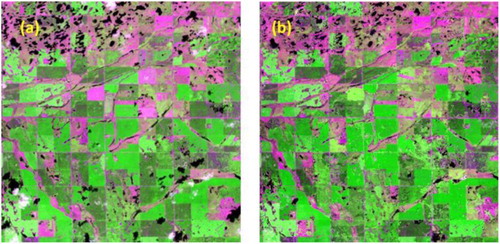
Table 3. The difference in surface reflectance between the Composite image and the Reference image.

	Band 1	Band 2	Band 3	Band 4	Band 5	Band 7
ME	0.00018	−0.00043	−0.00206	0.0034	0.0061	0.0038
MAE	0.0014	0.0055	0.0041	0.0217	0.0159	0.0094

The MODIS surface reflectance product is an appropriate data source to use as a reference because it provides high-quality data at a coarse resolution and is validated by independent field measurements (Jin et al. 2003). One benefit from this method is that the Landsat composite image is a MODIS-like surface reflectance. As such, MODIS algorithms for the retrieval of biophysical parameters could be directly applied to the Landsat composite image.

Since MODIS surface reflectances are consistently produced, the new method becomes feasible to produce a long-term time series of clear-sky Landsat composites which will greatly increase the applications of Landsat data. However, the selection of temporal resolution would depend on applications. In principle, the time interval should be long enough to collect sufficient clear-sky pixels over the area of interest, but short enough to capture the dynamic changes of the surface features. For example, Kross et al. (2011) found that the temporal resolution of less than 28 days is preferred for the start of growing season trends analysis of Boreal forests. Since the normalized images are MODIS-like surface reflectance images which are radiometrically consistent and comparable, the normalization technique used in this study is not only applicable to Landsat images but also to other medium resolution images from other optical sensors (e.g. SPOT, Sentinel). Therefore, our method is able to produce clear-sky composites from multi-sensor images. This is particularly useful to generate a composite for a short period to capture the dynamic changes of the surface features when available Landsat images are limited (e.g. the low latitude areas).

The performance of the proposed Landsat compositing method can be affected by two main factors: the accuracy of co-registration among images and the accuracy of cloud and cloud shadow detection. Accurate co-registration of images is critical in the radiometric normalization and the ‘best pixel’ selection. In the radiometric normalization process, accuracy of matching samples from Landsat TOA data and MODIS surface reflectance highly depends on the co-registration accuracy of the two images. Since the MODIS PSF is applied in the Landsat data resampling, a resampled Landsat pixel value is actually a weighted mean value of pixels within the actual observation area (the corresponding MODIS pixel) and pixels in the surrounding area with half-size of MODIS. The weights from the MODIS’s PSF are linearly decreasing from the observation center to the edge. The central pixel in the observation area has the highest weight and the edge pixels have the lowest weight. Therefore the resampled Landsat surface reflectance has a very small amount from pixels other than the MODIS pixel itself due to the PSF’s effect. Because each selected matching resampled Landsat pixel observes a homogeneous area with double-size of the MODIS pixel itself, a geo-referencing error may affect edge pixels of the observation, which contribute a very small amount to the resampled Landsat pixel value. Therefore, in this paper, the Landsat resampling strategy can reduce the effect of geo-referencing error between Landsat TOA and MODIS surface reflectance images. In the Landsat compositing processing, highly accurate geo-registration of the Landsat images is necessary since there is no appropriate way to reduce the effect of co-registration errors among the Landsat images.

In the radiometric normalization process, only cloud-free pixels in both Landsat and MODIS images are selected for the regression analysis. The compositing criteria highly depend on the cloud and cloud shadow masks derived from Landsat images. Therefore, an accurate cloud and cloud shadow mask is key to ensure a high performance of the new method. In this study, the MODIS cloud and cloud shadow information is from the MCD43A4 products. The Fmask algorithm was used to derive cloud and cloud shadow mask for each Landsat scene. Although both algorithms used for detecting clouds and cloud shadows in MODIS and Landsat images have high accuracy (Jin et al. 2003; Zhu and Woodcock 2012), the residual clouds (especially haze) and cloud shadows may still be measurable and may bring outliers to simple linear regression for building radiometric normalization models. To reduce their negative impacts to the compositing process, we used the Thiel–Sen regression in the radiometric normalization process due to its robustness to outliers resulting largely from the residual clouds and cloud shadows. We also introduced the b1 in compositing criteria which is especially sensitive to thin cloud and haze to further reduce the impact of cloud residuals in the composting process. All these processes enhance the detection of cloud/shadow over other land cover types in complex landscapes.

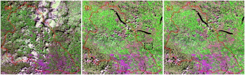
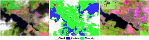
Although the method was tested on a landscape that mainly consisted of cropland, it is expected that the method can be extended to other landscapes such as urban, forest, and arctic tundra. As an example, a specific analysis was conducted for investigating the performance of this method applied to urban areas because urban areas might be easily confused with the cloud/shadow. In such a case, all subset images covering the urban areas in our study area were extracted, in which the cloud/shadow was visually interpreted as the references (true cloud/shadow maps). The comparison between the detected cloud/shadow and references showed that an accurate cloud/shadow detection over urban was achieved, with a commission error of 0.17 and an omission error of 0.09. The impact of these residual cloud/shadow errors can be further reduced in the image composition. Figure 6 shows an example of the cloud/shadow detection and the image compositing over an urban area, where (a) is the cloud-contaminated subset image of the Landsat-8 scene (32/26) acquired on 26 July 2013, (b) is the derived subset cloud/shadow mask, and (c) is the subset composite image from the combination of Landsat-7 and Landsat-8 images. From visually inspecting Figure 6(c), we found that a 100% cloud-free image over the urban was generated. However, more experiments on other landscapes and different season may be needed in future study.

Figure 6. Cloud/shadow detection and image compositing over an urban area: (a) the cloud-contaminated subset image (red: SWIR band, green: NIR band, blue: RED band) from the Landsat-8 scene (32/26) acquired on 26 July 2013; (b) the derived cloud/shadow mask; (c) the subset composite image (red: SWIR band, green: NIR band, blue: RED band) from the combination of Landsat-7 and Landsat-8 images.

5. Summary

This letter presents a new Landsat image compositing method for producing clear-sky images using all available cloud-contaminated Landsat-7 (SLC-Off) and Landsat-8 scenes, which were acquired in a short period. In this method, a Thiel–Sen regression-based normalization technique was developed to make the signals from different Landsat scenes radiometrically consistent and comparable. Comparing to the traditional normalization technique based on overlapped regions, this technique uses a MDOIS surface reflectance image as the reference and thus has the advantage of using the full Landsat scene to maximize the amount of samples in the regression analysis. Its merits also include: (1) reducing the effect of co-registration errors between Landsat and MODIS images on the Landsat radiometric normalization models; (2) minimizing the impact of potential misidentification of clouds and cloud shadows on the pixel-based compositing process. To enhance the pixel selection of land/water over cloud/shadow in the image compositing, we used pixel compositing criteria, which combined the modified maximum VI and the modified minimum visible reflectance selection methods. The proposed method was applied to a set of 13 Landsat-7 and Landsat-8 scenes acquired in the peak growing season of 2013 over an agriculturally dominated region, which resulted in a 95.8% cloud-free image. The composite well preserves the spectral characteristics of the original images. Therefore the method provides an efficient way for producing high-quality clear-sky Landsat images, which will increase the usability of contaminated Landsat data. It can also be used to produce long time series of Landsat composites. An another benefit of this method is that the final product is a MODIS-like surface reflectance image, thus suitable for retrieving biophysical parameters using available MODIS algorithms. The method can be extended to composite data from other medium resolution optical sensors (e.g. SPOT, AWiFS, ASTER, and Sentinel-2) using other coarse resolution data as a reference (e.g. SPOT/VEGETATION, AVHRR, and MERIS).

Acknowledgements

Authors gratefully thank Dr Vern Singhroy of the Canada Centre for Maping and Earth Observation for internally reviewing the article. Authors are also grateful to Ms Mary-Anne Fobert for careful editing of the manuscript. The editor and anonymous reviewers are also thanked for their valuable comments and suggestions, which improved an earlier version of this article. The manuscript was assigned the Natural Resources Canada (NRCan) contribution number 20150389.

Disclosure statement

No potential conflict of interest was reported by the authors.

Additional information

Funding

This work was supported by the Long Term Satellite Data Records Project and Groundwater Geoscience Program of NRCan.

References

- Chen, W., W. Chen, and J. Li. 2010. “Comparison of Surface Reflectance Derived by Relative Radiometric Normalization Versus Atmospheric Correction for Generating Large-Scale Landsat Mosaics.” Remote Sensing Letters 1 (2): 103–109. doi: 10.1080/01431160903518057
- Chen, W., B. Dominique, J. Li, K. Keohler, R. H. Fraser, Y. Zhang, S. G. Leblance, I. Olthof, J. Wang, and M. Mcgovern. 2009. “Biomass Measurements and Relationships with Landsat-7/ETM+ and JERS-1/SAR data over Canada's Western Sub-arctic and Low Arctic.” International Journal of Remote Sensing 30 (9): 2355–2376. doi: 10.1080/01431160802549401.
- Cihlar, J. 1996. “Identification of Contaminated Pixels in AVHRR Composite Images for Studies of Land Biosphere.” Remote Sensing of Environment 56 (3): 149–163. doi: 10.1016/0034-4257(95)00190-5
- Cihlar, J., and J. Howarth. 1994. “Detection and Removal of Cloud Contamination from AVHRR Images.” IEEE Transactions on Geoscience and Remote Sensing 32 (3): 583–589. doi: 10.1109/36.297976
- Du, Y., J. Cihlar, and R. Latifovic. 2001. “Radiometric Normalization, Compositing, and Quality Control for Satellite High Resolution Image Mosaics over Large Areas.” IEEE Transactions on Geoscience and Remote Sensing 39 (3): 623–634. doi: 10.1109/36.911119
- Gao, F., J. G. Masek, M. Schwaller, and F. Hall. 2006. “On the Blending of the Landsat and MODIS Surface Reflectance: Predict Daily Landsat Surface Reflectance.” IEEE Transactions on Geoscience and Remote Sensing 44 (8): 2207–2218. doi: 10.1109/TGRS.2006.872081
- Gao, F., J. G. Masek, R. E. Wolfe, and C. Huang. 2010. “Building a Consistent Medium Resolution Satellite Data Set Using Moderate Resolution Imaging Spectroradiometer Products as Reference.” Journal of Applied Remote Sensing 4 (1): 043526. doi: 10.1117/1.3507249
- Griffiths, P., S. van der Linden, T. Kuemmerle, and P. Hostert. 2013. “A Pixel-Based Landsat Compositing Algorithm for Large Area Land Cover Mapping.” IEEE Journal of Selected Topics in Applied Earth Observations and Remote Sensing 6 (5): 2088–2101. doi: 10.1109/JSTARS.2012.2228167
- Han, Y., B. Francesca, and W. H. Lee. 2017. “Automatic Cloud-Free Image Generation from High-Resolution Multitemporal Imagery.” Journal of Applied Remote Sensing 11 (2). doi:10.1117/1.JRS.11.025005.
- Huang, C., J. G. R. Townshend, S. Liang, S. N. V. Kalluri, and R. S. DeFries. 2002. “Impact of Sensor’s Point Spread Function on Land Cover Characterization: Assessment and Deconvolution.” Remote Sensing of Environment 80: 203–212. doi: 10.1016/S0034-4257(01)00298-X
- Hughes, M. J., and D. J. Hayes. 2014. “Automated Detection of Cloud and Cloud Shadow in Single-Date Landsat Imagery Using Neural Networks and Spatial Post-Processing.” Remote Sensing 6: 4907–4926. doi: 10.3390/rs6064907
- Jin, Y., C. B. Schaaf, C. E. Woodcock, F. Gao, X. Li, A. H. Strahler, W. Lucht, and S. Liang. 2003. “Consistency of MODIS Surface Bidirectional Reflectance Distribution Function and Albedo Retrievals: 2. Validation.” Journal of Geophysical Research 108 (D5): 2341. doi:10.1029/2002JD002804.
- Kross, A., R. Fernandes, J. Seaquist, and E. Beaubien. 2011. “The Effect of the Temporal Resolution of NDVI Data on Season Onset Dates and Trends Across Canadian Broadleaf Forests.” Remote Sensing of Environment 115 (6): 1564–1575. doi: 10.1016/j.rse.2011.02.015
- Leckie, D. 1990. “Advances in Remote Sensing Technologies for Forest Surveys and Management.” Canadian Journal of Forest Research 20 (4): 464–483. doi: 10.1139/x90-063
- Li, J., and W. Chen. 2007. “Clustering Synthetic Aperture Radar (SAR) Imagery Using an Automatic Approach.” Canadian Journal of Remote Sensing 33 (4): 303–311. doi: 10.5589/m07-032
- Li, J., and S. Wang. 2015. “An Automatic Method for Mapping Inland Surface Waterbodies with Radarsat-2 Imagery.” International Journal of Remote Sensing 36 (50): 1367–1384. doi: 10.1080/01431161.2015.1009653
- Lin, C., K. Lai, Z. Chen, and J. Chen. 2014. “ Patch-Based Information Reconstruction of Cloud-Contaminated Multitemporal Images.” IEEE Transactions on Geoscience and Remote Sensing 52 (1): 163–174. doi: 10.1109/TGRS.2012.2237408
- Lin, C.-H., P.-H. Tsai, K.-H. Lai, and J.-Y. Chen. 2013. “Cloud Removal from Multitemporal Satellite Images Using Information Cloning.” IEEE Transactions on Geoscience and Remote Sensing 51 (1): 232–241. doi: 10.1109/TGRS.2012.2197682
- Luo, Y., A. P. Trishchenko, and K. V. Khlopenkov. 2008. “Developing Clear-sky, Cloud and Cloud Shadow Mask for Producing Clear-sky Composites at 250-Meter Spatial Resolution for the Seven MODIS Land Bands over Canada and North America.” Remote Sensing of Environment 112 (12): 4167–4185. doi: 10.1016/j.rse.2008.06.010
- Martinuzzi, S., W. A. Gould, and O. M. Ramos Gonzalez. 2006. Creating Cloud-Free Landsat ETM+ Data Sets in Tropical Landscapes: Cloud and Cloud-Shadow Removal. General Technical Report, IITF-32. Rio Piedras: US Department of Agriculture, Forest Service, International Institute of Tropical Forestry. 12p.
- Olthof, I., D. Pouliot, R. Fernandes, and R. Latifovic. 2005. “Landsat-7 ETM+ Radiometric Normalization Comparison for Northern Mapping Applications.” Remote Sensing of Environment 95 (3): 388–398. doi: 10.1016/j.rse.2004.06.024
- Potapov, P., S. Turubanova, and M. C. Hansen. 2011. “Regional-scale Boreal Forest Cover and Change Mapping Using Landsat Data Composites for European Russia.” Remote Sensing of Environment 115: 548–561. doi: 10.1016/j.rse.2010.10.001
- Roy, P., J. Ju, K. Kline, P. L. Scaramuzza, V. Kovalskyy, M. Hansen, T. R. Loveland, E. Vermote, and C. Zhang. 2010. “Web-enabled Landsat Data (WELD): Landsat ETM+ Composited Mosaics of the Conterminous United States.” Remote Sensing of Environment, 114: 35–49. doi:10.1016/j.rse.2009.08.011.
- Simpson, J. J., and J. R. Stitt. 1998. “A Procedure for the Detection and Removal of Cloud Shadow from AVHRR Data over Land.” IEEE Transactions on Geoscience and Remote Sensing 36 (3): 880–897. doi: 10.1109/36.673680
- Tan, B., C. E. Woodcock, J. Hu, P. Zhang, M. Ozdogan, D. Huang, W. Yang, Y. Knyazikhin, and R. B. Myneni. 2006. “The Impact of Gridding Artifacts on the Local Spatial Properties of MODIS Data: Implications for Validation, Compositing, and Band-to-Band Registration Across Resolutions.” Remote Sensing of Environment 105 (2): 98–114. doi: 10.1016/j.rse.2006.06.008
- Teillet, P. M., J. L. Barker, B. L. Markham, R. R. Irish, G. Fedosejevs, and J. C. Storey. 2001. “Radiometric Cross-Calibration of the Landsat-7 ETM+ and Landsat-5 TM Sensors Based on Tandem Data Sets.” Remote Sensing of Environment 78 (1): 39–54. doi: 10.1016/S0034-4257(01)00248-6
- Wang, S. 2008. “Simulation of Evapotranspiration and its Response to Plant Water and CO2 Transfer Dynamics.” Journal of Hydrometeorology 9 (3): 426–443. doi: 10.1175/2007JHM918.1
- Wang, S., Y. Yang, Y. Luo, and A. Rivera. 2013. “Spatial and Seasonal Variations in Evapotranspiration over Canada’s Landmass.” Hydrology and Earth System Sciences 17 (9): 3561–3575. doi: 10.5194/hess-17-3561-2013
- Xu, M., X. Jia, M. Pickering, and A. J. Plaza. 2016. “Cloud Removal Based on Sparse Representation via Multitemporal Dictionary Learning.” IEEE Transactions on Geoscience and Remote Sensing 54 (5): 2998–3006. doi: 10.1109/TGRS.2015.2509860
- Zhou, F., and A. Zhang. 2013. “Methodology for Estimating Availability of Cloud-Free Image Composites: A Case Study for Southern Canada.” International Journal of Applied Earth Observation and Geoinformation 21 (1): 17–31. doi: 10.1016/j.jag.2012.07.017
- Zhu, Z., and C. E. Woodcock. 2012. “Object-Based Cloud and Cloud Shadow Detection in Landsat Imagery.” Remote Sensing of Environment 118 (1): 83–94. doi: 10.1016/j.rse.2011.10.028