3D Surface velocity retrieval of mountain glacier using an offset tracking technique applied to ascending and descending SAR constellation data: a case study of the Yiga Glacier

ABSTRACT

COSMO-SkyMed is a constellation of four X-band high-resolution radar satellites with a minimum revisit period of 12 hours. These satellites can obtain ascending and descending synthetic aperture radar (SAR) images with very similar periods for use in the three-dimensional (3D) inversion of glacier velocities. In this paper, based on ascending and descending COSMO-SkyMed data acquired at nearly the same time, the surface velocity of the Yiga Glacier, located in the Jiali County, Tibet, China, is estimated in four directions using an offset tracking technique during the periods of 16 January to 3 February 2017 and 1 February to 19 February 2017. Through the geometrical relationships between the measurements and the SAR images, the least square method is used to retrieve the 3D components of the glacier surface velocity in the eastward, northward and upward directions. The results show that applying the offset tracking technique to COSMO-SkyMed images can be used to derive the true 3D velocity of a glacier’s surface. During the two periods, the Yiga Glacier had a stable velocity, and the maximum surface velocity, 2.4 m/d, was observed in the middle portion of the glacier, which corresponds to the location of the steepest slope.

KEYWORDS:

• Mountain glacier
• inversion of 3D movement
• offset tracking
• SAR constellation data

1. Introduction

As an important type of glacier, mountain glaciers are often regarded as sensitive recorders and indicators of global climate change (Quincey, Luckman, and Benn 2009). Additionally, glacier movement, one of the most important features of glaciers, can cause serious natural disasters, such as debris flow and glacial lake outburst floods, that threaten human production and life (Bolch et al. 2008). Thus, monitoring glacier movement has great significance for predicting glacial flow and hazards (Haemmig et al. 2014). However, mountain glaciers are generally located in harsh natural environments, making it difficult to conduct regular and large-scale field monitoring. The emergence of remote sensing, especially synthetic aperture radar (SAR), has provided available means to monitor glacier variation in a routine, low-cost, high-frequency and large spatial coverage manner (Mouginot et al. 2017).

SAR can be used to acquire images both during the day and at night, as well as in any weather conditions (Rignot and Mouginot 2012). Consequently, SAR has become an invaluable tool for glacier research (Strozzi et al. 2002; Mouginot, Scheuchl, and Rignot 2012). Several methods based on SAR images can be currently used to measure glacier velocity: the differential SAR interferometry (DInSAR) and multiple aperture interferometric (MAI) techniques use SAR phase information, and the offset tracking technique uses amplitude information (Mohr, Reeh, and Madsen 2003; Hu et al. 2014; Sánchez-Gámez and Navarro 2017). The DInSAR and MAI techniques are able to measure deformations in line-of sight (LOS) and azimuth directions, respectively, and can yield accuracies on the centimetre to even sub-centimetre scale (Goldstein et al. 1993; Bechor and Zebker 2006). However, the two methods are always limited by loss of coherence, which is easily affected by the large temporal baselines of SAR image pairs or glacier velocities that are too high (Strozzi et al. 2002; Bechor and Zebker 2006). The accuracy of the offset tracking technique is generally lower than that of the DInSAR and MAI techniques and has a range from 1/10 to 1/30 pixels (Strozzi et al. 2002; Riveros et al. 2013). However, this technique is rarely affected by decorrelation and can be used to directly estimate displacement in both LOS and azimuth directions (Gray et al. 1998; Yan 2013).

Although many monitoring studies have been conducted on glacier velocity using the three techniques, few studies have performed 3D surface velocity inversions of mountain glaciers (Rignot and Kanagaratnam 2006; Satyabala 2016; Tong et al. 2018). Due to the limitations of SAR data, a method that uses a high-precision digital elevation model (DEM) to retrieve the 3D glacier field (with the assumption that the glacier flow direction is parallel to the surface of the glacier) has been put forward and has had some achievements (Joughin, Kwok, and Fahnestock 1998; Strozzi et al. 2002; Kumar, Venkataramana, and Høgda 2011). However, to estimate the true 3D movement, at least three SAR measurements in quite different directions are required (Wright, Parsons, and Lu 2004). With the launch of modern advanced radar satellites, especially satellite constellations, it has become possible to acquire ascending and descending passes of SAR data for the same area, and reliable 3D velocity retrieval of glaciers can be realized (Neelmeijer, Motagh, and Wetzel 2014; Sánchez-Gámez and Navarro 2017). For example, based on PALSAR, ENVISAT and ASAR data, Ju Hu et al. successfully estimated the 3D movement of Dongkemadi Glacier on the Qinghai-Tibetan Plateau by integrating the results of DInSAR, MAI and offset tracking (Hu et al. 2014). Gray estimated the full 3D movement of Henrietta Nesmith Glacier, Canada, using multiple RADARSAT-2 InSAR pairs with different incidence angles and orbital directions (Gray 2011). In fact, the offset tracking technique can obtain the LOS and azimuth displacements. Combining the offset tracking results for the four directions of the ascending and descending data, it is possible to directly invert the true flow of the glacier surface by using just the offset tracking technique. Although it is not as accurate as the DInSAR and MAI technique, the offset tracking technique has a particular advantage in that it can generate robust deformation results even if the coherence is poor (Strozzi et al. 2002, 2008).

Developed by the Italian Space Agency and the Italian Ministry of Defence, COSMO-SkyMed includes four satellites, each of which is equipped with a high-resolution SAR instrument. The revisit time of the constellation can be less than 12 hours, which provides the possibility of acquiring ascending and descending SAR images in the same area during almost the same period (Covello et al. 2010). In this paper, eastward, northward and upward projections of the surface velocity of the Yiga Glacier in the Nyainqentanglha Mountains, China, are calculated using the offset tracking technique applied to ascending and descending COSMO-SkyMed images, and the results demonstrate the feasibility of using COSMO-SkyMed data to invert the 3D movement of glaciers. A detailed analysis of the glacial flow characteristics is also provided.

2. Study area and data sources

The Yiga Glacier is located in Jiali County, Tibet, China, centred at 30.315° N and 93.579° E (shown in Figure 1). According to The Second Glacier Inventory Dataset of China, its altitude ranges from 3862.5 to 6606.9 m, with an average elevation of 5450.6 m (Liu et al. 2014). The largest elevation difference is nearly 3000 m. The glacier and the Niduzangbu River intersect at the glacier terminus, and the river flows over glacial debris. The movement of the Yiga Glacier can directly affect the flow direction and water level of the Niduzangbu River. Moreover, there are several villages within two kilometres downstream. Monitoring the Yiga Glacier’s movement is significant for the safety of these villages.

Figure 1. Data coverage and location of the Yiga Glacier.

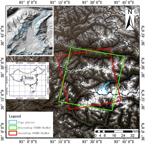
Glacier surface velocity is closely related to time. To ensure the reliability of the 3D inversion, ascending and descending SAR images should be acquired over almost the same period (Fallourd et al. 2010). As a constellation with four satellites, COSMO-SkyMed has a short revisit time. This short revisit time is in part why the COSMO-SkyMed data are used in this paper. The temporal distance between the ascending and descending images is only 1 day, 12 hours, and 11 minutes, which can be regarded as nearly the same period. The SAR images also have a high resolution, with HH polarization mode and HImage acquisition mode. The details of the offset tracking pairs are listed in Table 1. Due to the small time difference, the glacier can be considered to have the same velocity during the ascending period and the descending period. Thus, from 16 January to 3 February and from 1 February to 19 February 2017, four different measurements from offset tracking applied to ascending and descending SAR pairs can be exploited to calculate reliable 3D movements in each period. To remove the offset caused by topography in the offset tracking technique, the 5 × 5 m high-resolution DEM generated from TanDEM-X is used in this paper.

Table 1. Details of COSMO-SkyMed image pairs used for the Yiga Glacier 3D movement retrieval.

No.	Reference Image Date	Slave Image Date	${\text{B}}_{\mathrm{\perp }}$(m)	Time Baseline (d)	Azimuth (m) × Slant-range (m)	Ascending/Descending
1	2017/01/16	2017/01/31	40.2	15	2.3 × 1.0	Ascending
	2017/01/18	2017/02/03	−37.1	16	2.2 × 0.9	Descending
2	2017/02/01	2017/02/17	−92.1	16	2.3 × 1.0	Ascending
	2017/02/03	2017/02/19	98.3	16	2.2 × 0.9	Descending

3. Method

3.1. Offset tracking technique

As the core of the offset tracking technique, the normalized cross-correlation algorithm is used to calculate offset fields based on the intensity information of SAR images (Gray et al. 1998; Strozzi et al. 2002; Huang and Li 2011; Zhou, Li, and Guo 2014). The key is to select a reference window in the master image and match it with a search window in the slave image by calculating a maximum cross-correlation coefficient. Then, a local total offset is estimated (Yan et al. 2015). In general, the total offset contains four primary components: the offset caused by glacier movement, the offset caused by the difference in satellite orbit position, the offset associated with the ionosphere and the offset induced by topography (Yan et al. 2013). Assuming that deformation in non-glacier areas in the image is zero, the least square method can be used to fit the offset polynomial according to the SAR orbital parameters to calculate the orbital offset (Strozzi et al. 2008). The ionosphere offset is always ignored in mid- or low-latitude regions (Wegmueller et al. 2006). In the azimuth direction, the topography-related offset is related to the horizontal crossing angle of the two satellite orbits, the look angle of the SAR images, the topographic (vertical) error and the azimuth pixel spacing, whereas in the slant-range direction, it is related to the perpendicular baseline value, the slant range value, the look angle, the topographic (vertical) error and the slant-range pixel spacing (Sansosti et al. 2006; Yan et al. 2013). When the terrain is flat and the perpendicular baseline of the SAR pairs is small, the topography-related offset is often negligible (Deng et al. 2015).

In this paper, the study area is located in rugged terrain on the Qinghai-Tibet Plateau, so the offset caused by topography cannot be ignored. According to the parameter information of an ascending COSMO-SkyMed image used in this study, the look angle is 26°; the azimuth pixel spacing and slant-range pixel spacing are approximately 1.0 and 2.3 m, respectively; and the slant range value is approximately 620 km. The horizontal crossing angle is theoretically zero from the COSMO constellation nominal configuration (Covello et al. 2010). In fact, it is not precisely zero but is small enough that it can be ignored. Based on the above, there is no offset in the azimuth direction caused by topography. However, in the slant-range direction, assuming a perpendicular baseline value of 100 m, the slant-range offset would exceed 1/8 of a pixel without the use of an external DEM. Therefore, the offset induced by topography here cannot be neglected. The DEM in this paper generated from TanDEM-X has a high-resolution of 5 m and can be used to calculate a more accurate topography offset than the widely used Shuttle Radar Topography Mission (SRTM) DEM.

After removing the offset caused by topography, only the glacier displacement remains. Through repeated experiments and comparative analysis, this study found that setting an offset tracking window size of 100 × 100 pixels, corresponding to the area of approximately 300 × 300 m on the ground, not only preserves the details of glacier motion but also makes motion information more continuous. To acquire high-resolution results, the matching steps applied in the slant-range direction and azimuth direction are both 1 pixel, despite the time costs. Additionally, values of the cross-correlation coefficient lower than 0.1 are rejected.

3.2. Inversion of 3D movement field

By applying the offset tracking technique to ascending and descending passes of SAR data, displacement vectors in four directions, i.e. ascending LOS measurements $d_{los}^a$, ascending azimuth measurements $d_{az}^a$, descending LOS measurements $d_{los}^d$ and descending azimuth measurements $d_{az}^d$, can be obtained. By projecting the true displacement of the glacier surface to the eastward, northward and upward directions, the corresponding displacements $d_E$, $d_N$ and $d_U$ are obtained (Fallourd et al. 2010). Moreover, the LOS displacement is the sum of the elements from the three displacements projected to the LOS direction. The azimuth displacement is the sum of the elements from the three displacements projected to the azimuth direction. For the COSMO-SkyMed images used in this paper, the orbital azimuth angle of the ascending reference images is 349.22°, and that of the descending images is 191.08°. ${\theta }^a$, which is the incidence angle of each pixel in the ascending reference image, ranges from 30.64° to 31.44°, and ${\theta }^d$, which is the incidence angle of each pixel in the descending reference image, ranges from 26.26° to 27.12°. Combined with the imaging geometry of the SAR satellite, several equations can be written as follows:(1) $d_{los}^a=(d_N\sin {349.22}^{\circ }-d_E\cos {349.22}^{\circ })\sin {\theta }^a+d_U\cos {\theta }^a$(1) (2) $d_{los}^d=(d_N\sin {191.08}^{\circ }-d_E\cos {191.08}^{\circ })\sin {\theta }^d+d_U\cos {\theta }^d$(2) (3) $d_{az}^a=d_N\cos {349.22}^{\circ }+d_E\sin {349.22}^{\circ }$(3) (4) $d_{az}^d=d_N\cos {191.08}^{\circ }+d_E\sin {191.08}^{\circ }$(4)

The above four equations can be formulated for each pixel in the overlapping area. Let(5) $D=[d_{los}^a{d}_{los}^d{d}_{az}^a{d}_{az}^d{]}^T$(5) (6) $X=[d_U{d}_N{d}_E{]}^T$(6) (7) $C=\left[\begin{array}{ccc}\cos {\theta }^a& \sin {349.22}^{\circ }\sin {\theta }^a& -\cos {349.22}^{\circ }\sin {\theta }^a\\ \cos {\theta }^d& \sin {191.08}^{\circ }\sin {\theta }^d& -\cos {191.08}^{\circ }\sin {\theta }^d\\ 0& \cos {349.22}^{\circ }& \sin {349.22}^{\circ }\\ 0& \text{cos}{191.08}^{\circ }& \sin {191.08}^{\circ }\end{array}\right]$(7)

The four equations above can be written as:(8) $D=CX$(8) Then, the $d_U,d_N$ and $d_E$ can be solved using the least square method.

Because of the orbital azimuth angle differences between ascending and descending COSMO-SkyMed data, the shadow and layover regions of the offset tracking results have different distributions. Masking all these regions is necessary to prevent them from being used for the 3D inversion of glacier movement. In addition, only the zones above the correlation threshold have displacement results. The scope of the displacement results in the ascending SAR pair is different from the descending SAR pair. Thus, 3D movement calculated should be in the common area. After the above steps, the 3D movement field of the remaining area can be considered reliable.

4. Results and analysis

4.1. Analysis of 3D movement

After applying the offset tracking technique to SAR image pairs and calculating the 3D movement, two sets of 3D movement fields were obtained for the Yiga Glacier, as shown in Figure 2.

Figure 2. The 3D velocity components in the east-west, north-south and up-down directions during the two periods of 16 January to 3 February 2017 ((a), (b) and (c)) and 1 February to 19 February 2017 ((d), (e) and (f)).

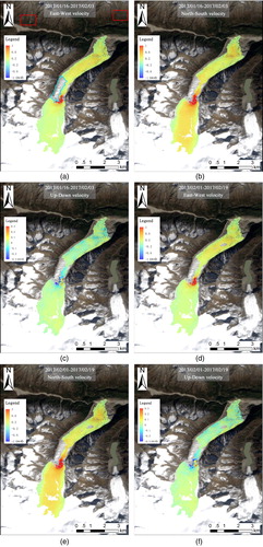
The 3D velocity components above show several features. (1) In most of the accumulation area of the Yiga glacier and a blue polygonal area shown in Figure 2(a), there are no glacier displacement results. In the accumulation area, the lack of surface features means that the offset tracking technique performs poorly. In the blue polygonal area, the layover exists in that area in the descending COSMO-SkyMed images; thus, it cannot be used to conduct inversion of the 3D movement field. (2) The maximum values of the three components of 3D velocity all exist in the middle of the Yiga Glacier, which may be related to the large slope in this region. (3) Between the two periods, the distributions of the three components in the eastward, northward and upward directions have a high consistency. (4) According to Figure 2(a,d), for the eastern component, the velocity is obviously larger in the lower middle portion of the Yiga Glacier than in the upper middle portion. According to Figure 2(b,e), for the northern component, the velocity is obviously lower in the lower middle part of the Yiga Glacier than in the upper middle part. This pattern is related to the orientation of the Yiga Glacier: the upper middle portion is oriented towards the north, and the lower middle portion is oriented towards the northeast. (5) The maximum variation in the upward velocity is distributed in the middle portion, with a negative value in the western half part and a positive value in the eastern half part (Figure 2(c,f)). This uplift phenomenon may be due to a sudden change in the glacier flow direction here, resulting in squeezing of the eastern half part of the middle portion.

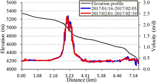
To better analyse the surface velocity of the Yiga Glacier, the three components of the 3D velocity are synthesized, and the synthetic direction of the east–west and north–south components is taken as the flow direction of the glacier surface. Synthetic 3D velocity values in m/day are shown in Figure 3, and small black arrows represent the synthetic direction. Then, a profile along the central line of the glacier, shown in Figure 3(a), is selected, and the relation between velocity pattern and elevation change along the profile is revealed, as shown in Figure 4. The horizontal axis represents the distance along the profile from point A to B. The primary vertical axis represents elevation, measured in metres. The secondary vertical axis represents the 3D velocity value in m/day. Several observations can be made after analysing the displacement results: (1) The directions of the black arrows, which are calculated from the ratio of the eastern velocity component to the northern velocity component, are highly consistent with the direction of the Yiga Glacier, which shows that the solution of the 3D velocity in this paper is reliable. (2) The 3D velocity patterns have similar distributions in Figure 3(a,b). In addition, the two sets of 3D velocity curves in Figure 4 coincide well. Thus, the Yiga Glacier is considered to have a stable velocity from 16 January to 19 February 2017. (3) The synthetic velocity along the profile changes with elevation. From 0 to 2 km and 4.05 to 6.8 km, the altitude decreases smoothly, and the glacier has a slow and steady velocity of approximately 0.4 m/day. From 2 to 2.60 km, the velocity increases to 0.58 m/day because of a slight increase in the slope, and from 3.55 to 4.05 km, the velocity decreases steadily to 0.4 m/d because of a slight decrease in the slope. From 2.60 to 3.55 km, the velocities in the two periods both suddenly increase to 2.4 m/d then suddenly decrease to 0.75 m/day with a rapid decrease in altitude. Then, at distances greater than 6.8 km, the glacier velocity increases slightly because of a slight increase in the slope. Overall, the velocity trend of the Yiga Glacier is in good agreement with the elevation trend.

Figure 3. 3D velocity of the Yiga Glacier in two periods.

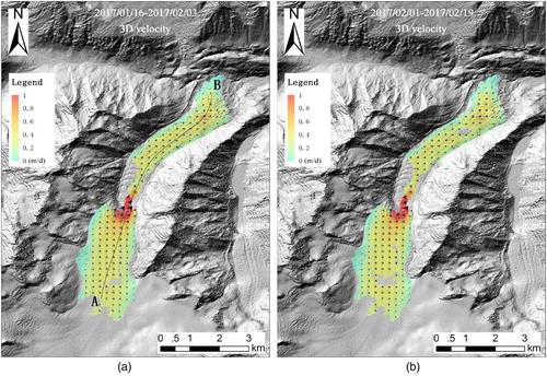
Figure 4. Velocity profiles of the Yiga Glacier in two periods and elevation variation along the profile.

4.2. Error analysis

Errors in the offset tracking results are mainly caused by SAR image registration, geocoding and topography (Li et al. 2013). A high-accuracy external DEM can minimize the error contributed by topography and help achieve high-precision registration of SAR images in complex terrain. The residual error due to image co-registration and rugged terrain in this paper is approximately 1/15 pixels, which is approximately 20 cm per time baseline in terms of COSMO-SkyMed. For the synthesized 3D velocity of the Yiga Glacier, the error contribution is approximately 1.5 cm/d on average. The Yiga Glacier is located between two towering mountains with hostile environments and blocked roads in winter, which makes it difficult to measure the velocity by field survey. According to the assumption that the displacement of the non-ice region is zero theoretically, the accuracy of the glacier velocity estimates can be evaluated using the root mean square error (RMSE) of residual displacement in the non-ice region (Yan 2013). Several areas are selected to calculate the residual displacement velocity of the three components and the synthesized 3D velocity (as shown by the two red rectangles in Figure 2(a)). For the first group, the RMSEs are 0.67, 0.95 and 0.22 cm/d for the eastward, northward and upward components, respectively, and 1.18 cm/d for the synthetic velocity. In addition, for the second group, the RMSEs are 0.88, 1.43 and 0.32 cm/d for the eastward, northward and upward components, respectively, and 1.71 cm/d for the synthetic velocity. Clearly, these values are all much lower than the velocity of the Yiga Glacier, which indicates the good quality of the 3D velocity inversion.

5. Conclusions

In this study, the offset tracking technique has been used to invert the 3D velocity of the Yiga Glacier in the Nyainqentanglha Mountains, China, by applying it to ascending and descending COSMO-SkyMed images that have almost the same period. Four conclusions can be drawn. First, by applying the offset tracking technique to the intensity information of ascending and descending passes of SAR images and combining the four measurements with different directions, the 3D velocity field of glaciers can be estimated. Second, as a constellation with four radar satellites, COSMO-SkyMed has a short revisit time that can acquire ascending and descending images with very similar time periods. This technique has great potential to validate the true 3D velocity of glaciers using different image pairs mapping the same deformation field. Third, the Yiga Glacier had a stable velocity during the observation period from 16 January to 19 February 2017. The distribution of the glacier surface velocity is related to the elevation change. A maximum velocity of approximately 2.4 m/d is observed in the middle part of the glacier because the steepest slope is located there. With steadily decreasing elevation, the velocity in the upper middle and the lower middle portions of the Yiga Glacier stabilizes at approximately 40 cm/d. Finally, the low RMSE in the non-ice region indicates that the results in this paper are reliable.

Acknowledgements

The COSMO-SkyMed data employed in this study were provided by the Italian Space Agency, and the TanDEM-X data were provided by DLR.

Disclosure statement

No potential conflict of interest was reported by the authors.

ORCID

Jinghui Fan http://orcid.org/0000-0002-8243-5731

Guang Liu http://orcid.org/0000-0001-8596-8528

Additional information

Funding

This work was supported by the China Geological Survey under grant number [DD20160342], the China MOST-ESA Dragon Project - 4 under grant number [32365] and the National Science Foundation of China (NSFC) under grant number [41590852, 41001264].

References

- Bechor, Noa B. D., and Howard A. Zebker. 2006. “Measuring Two-Dimensional Movements Using a Single InSAR Pair.” Geophysical Research Letters 33 (16): 275–303. doi:10.1029/2006gl026883.
- Bolch, T., M. F. Buchroithner, J. Peters, M. Baessler, and S. Bajracharya. 2008. “Identification of Glacier Motion and Potentially Dangerous Glacial Lakes in the Mt. Everest Region/Nepal Using Spaceborne Imagery.” Natural Hazards and Earth System Science 8 (6): 1329–1340. doi: 10.5194/nhess-8-1329-2008
- Covello, F., F. Battazza, A. Coletta, E. Lopinto, C. Fiorentino, L. Pietranera, G. Valentini, and S. Zoffoli. 2010. “COSMO-SkyMed an Existing Opportunity for Observing the Earth.” Journal of Geodynamics 49 (3–4): 171–180. doi:10.1016/j.jog.2010.01.001.
- Deng, Fanghui, Chunxia Zhou, Zemin Wang, E. Dongchen, and Xin Zhang. 2015. “Ice-Flow Velocity Derivation of the Confluence Zone of the Amery Ice Shelf Using Offset-Tracking Method.” Geomatics and Information Science of Wuhan University 40 (7): 901–906.
- Fallourd, Renaud, Flavien Vernier, Yajing Yan, Emmanuel Trouvé, and Philippe Bolon. 2010. “Alpine Glacier 3D Displacement Derived From Ascending and Descending TerraSAR-X Images on Mont-Blanc Test Site.” 8th European conference on synthetic aperture radar (EUSAR 2010): 1–4.
- Goldstein, Richard M., Hermann Engelhardt, Barclay Kamb, and Richard M. Frolich. 1993. “Satellite Radar Interferometry for Monitoring Ice Sheet Motion: Application to an Antarctic Ice Stream.” Science 262 (5139): 1525–1530. doi: 10.1126/science.262.5139.1525
- Gray, Laurence. 2011. “Using Multiple RADARSAT InSAR Pairs to Estimate a Full Three-Dimensional Solution for Glacial Ice Movement.” Geophysical Research Letters 38 (5). doi:10.1029/2010gl046484.
- Gray, A. L., K. E. Mattar, P. W. Vachon, R. Bindschadler, K. C. Jezek, R. Forster, and J. P. Crawford. 1998. “InSAR Results from the RADARSAT Antarctic Mapping Mission Data: Estimation of Glacier Motion Using a Simple Registration Procedure.” Geoscience and remote sensing symposium proceedings, 1998. IGARSS ‘98. 1998 IEEE International 3:1638–40.
- Haemmig, Christoph, Matthias Huss, Hansrudolf Keusen, Josef Hess, Urs Wegmüller, Zhigang Ao, and Wubuli Kulubayi. 2014. “Hazard Assessment of Glacial Lake Outburst Floods from Kyagar Glacier, Karakoram Mountains, China.” Annals of Glaciology 55 (66): 34–44. doi:10.3189/2014AoG66A001.
- Hu, Jun, Zhiwei Li, Jia Li, Lei Zhang, Xiaoli Ding, Jianjun Zhu, and Qian Sun. 2014. “3-D Movement Mapping of the Alpine Glacier in Qinghai-Tibetan Plateau by Integrating D-InSAR, MAI and Offset-Tracking: Case Study of the Dongkemadi Glacier.” Global and Planetary Change 118: 62–68. doi:10.1016/j.gloplacha.2014.04.002.
- Huang, Lei, and Zhen Li. 2011. “Comparison of SAR and Optical Data in Deriving Glacier Velocity with Feature Tracking.” International Journal of Remote Sensing 32 (10): 2681–2698. doi: 10.1080/01431161003720395
- Joughin, Ian R., Ronald Kwok, and Mark Fahnestock. 1998. “Interferometric Estimation of Three-Dimensional ice-Flow Using Ascending and Descending Passes.” IEEE Transactions on Geoscience and Remote Sensing 36 (1): 25–37. doi:10.1109/36.655315.
- Kumar, V., G. Venkataramana, and K. A. Høgda. 2011. “Glacier Surface Velocity Estimation Using SAR Interferometry Technique Applying Ascending and Descending Passes in Himalayas.” International Journal of Applied Earth Observation & Geoinformation 13 (4): 545–551. doi:10.1016/j.jag.2011.02.004.
- Li, Jia, Zhiwei Li, Jianjun Zhu, Xiaoli Ding, Changcheng Wang, and Jianli Chen. 2013. “Deriving Surface Motion of Mountain Glaciers in the Tuomuer-Khan Tengri Mountain Ranges from PALSAR Images.” Global and Planetary Change 101: 61–71. doi:10.1016/j.gloplacha.2012.12.004.
- Liu, Shiyin, Wanqin Guo, Junli Xu, Donghui ShangGuan, Lizong Wu, Xiaojun Yao, Jingdong Zhao, et al. 2014. “The Second Glacier Inventory Dataset of China (Version 1.0).” Cold and Arid Regions Science Data Center at Lanzhou. doi:10.3972/glacier.001.2013.db.
- Mohr, Johan Jacob, Niels Reeh, and Søren Nørvang Madsen. 2003. “Accuracy of Three-Dimensional Glacier Surface Velocities Derived from Radar Interferometry and Ice-Sounding Radar Measurements.” Journal of Glaciology 49 (165): 210–222. doi:10.3189/172756503781830791.
- Mouginot, Jeremie, Eric Rignot, Bernd Scheuchl, and Romain Millan. 2017. “Comprehensive Annual Ice Sheet Velocity Mapping Using Landsat-8, Sentinel-1, and RADARSAT-2 Data.” Remote Sensing 9 (12): 364. doi:10.3390/rs9040364.
- Mouginot, Jeremie, Bernd Scheuchl, and Eric Rignot. 2012. “Mapping of Ice Motion in Antarctica Using Synthetic-Aperture Radar Data.” Remote Sensing 4 (12): 2753–2767. doi:10.3390/rs4092753.
- Neelmeijer, Julia, Mahdi Motagh, and Hans-Ulrich Wetzel. 2014. “Estimating Spatial and Temporal Variability in Surface Kinematics of the Inylchek Glacier, Central Asia, Using TerraSAR-X Data.” Remote Sensing 6 (10): 9239–9259. doi:10.3390/rs6109239.
- Quincey, D. J., A. Luckman, and D. Benn. 2009. “Quantification of Everest Region Glacier Velocities Between 1992 and 2002, Using Satellite Radar Interferometry and Feature Tracking.” Journal of Glaciology 55 (192): 596–606. doi: 10.3189/002214309789470987
- Rignot, Eric, and Pannir Kanagaratnam. 2006. “Changes in the Velocity Structure of the Greenland Ice Sheet.” Science 311 (5763): 986–990. doi: 10.1126/science.1121381
- Rignot, Eric, and Jeremie Mouginot. 2012. “Ice Flow in Greenland for the International Polar Year 2008-2009.” Geophysical Research Letters 39 (11). doi:10.1029/2012gl051634.
- Riveros, N., L. Euillades, P. Euillades, S. Moreiras, and S. Balbarani. 2013. “Offset Tracking Procedure Applied to High Resolution SAR Data on Viedma Glacier, Patagonian Andes, Argentina.” Advances in Geosciences 35: 7–13. doi:10.5194/adgeo-35-7-2013.
- Sánchez-Gámez, Pablo, and Francisco J. Navarro. 2017. “Glacier Surface Velocity Retrieval Using D-InSAR and Offset Tracking Techniques Applied to Ascending and Descending Passes of Sentinel-1 Data for Southern Ellesmere Ice Caps, Canadian Arctic.” Remote Sensing 9 (5): 422. doi:10.3390/rs9050442 doi: 10.3390/rs9050422
- Sansosti, Eugenio, Paolo Berardino, Michele Manunta, Francesco Serafino, and Gianfranco Fornaro. 2006. “Geometrical SAR Image Registration.” IEEE Transactions on Geoscience and Remote Sensing 44 (10): 2861–2870. doi:10.1109/tgrs.2006.875787.
- Satyabala, S. P. 2016. “Spatiotemporal Variations in Surface Velocity of the Gangotri Glacier, Garhwal Himalaya, India: Study Using Synthetic Aperture Radar Data.” Remote Sensing of Environment 181: 151–161. doi:10.1016/j.rse.2016.03.042.
- Strozzi, Tazio, Alexei Kouraev, Andreas Wiesmann, Urs Wegmüller, Aleksey Sharov, and Charles Werner. 2008. “Estimation of Arctic Glacier Motion with Satellite L-Band SAR Data.” Remote Sensing of Environment 112 (3): 636–645. doi:10.1016/j.rse.2007.06.007.
- Strozzi, Tazio, Adrian Luckman, Tavi Murray, Urs Wegmüller, and Charles L. Werner. 2002. “Glacier Motion Estimation Using SAR Offset-Tracking Procedures.” IEEE Transactions on Geoscience and Remote Sensing 40 (11): 2384–2391. doi:10.1109/tgrs.2002.805079.
- Tong, Xiaohua, Shuang Liu, Rongxing Li, Huan Xie, Shijie Liu, Gang Qiao, Tiantian Feng, Yixiang Tian, and Zhen Ye. 2018. “Multi-track Extraction of Two-Dimensional Surface Velocity by the Combined Use of Differential and Multiple-Aperture InSAR in the Amery Ice Shelf, East Antarctica.” Remote Sensing of Environment 204: 122–137. doi:10.1016/j.rse.2017.10.036.
- Wegmueller, Urs, Charles Werner, Tazio Strozzi, and Andreas Wiesmann. 2006. “Ionospheric Electron Concentration Effects on SAR and INSAR.” 2006 IEEE International Geoscience and Remote Sensing Symposium 1-8: 3731–3734. doi:10.1109/igarss.2006.956.
- Wright, Tim J., Barry E. Parsons, and Zhong Lu. 2004. “Toward Mapping Surface Deformation in Three Dimensions Using InSAR.” Geophysical Research Letters 31 (1): 169. doi:10.1029/2003gl018827.
- Yan, Shiyong. 2013. “Research on Extraction of Alpine Glacier Surface Movement by SAR Remote Sensing.”
- Yan, Shiyong, Huadong Guo, Guang Liu, and Zhixing Ruan. 2013. “Mountain Glacier Displacement Estimation Using a DEM-Assisted Offset Tracking Method with ALOS/PALSAR Data.” Remote Sensing Letters 4 (5): 494–503. doi:10.1080/2150704x.2012.754561.
- Yan, Shiyong, Guang Liu, Yunjia Wang, Zbigniew Perski, and Zhixing Ruan. 2015. “Glacier Surface Motion Pattern in the Eastern Part of West Kunlun Shan Estimation Using Pixel-Tracking with PALSAR Imagery.” Environmental Earth Sciences 74 (3): 1871–1881. doi:10.1007/s12665-015-4645-7.
- Zhou, Jianmin, Zhen Li, and Wanqin Guo. 2014. “Estimation and Analysis of the Surface Velocity Field of Mountain Glaciers in Muztag Ata Using Satellite SAR Data.” Environmental Earth Sciences 71 (8): 3581–3592. doi:10.1007/s12665-013-2749-5.