Exposing the urban continuum: implications and cross-comparison from an interdisciplinary perspective

ABSTRACT

There is an increasing availability of geospatial data describing patterns of human settlement and population such as various global remote-sensing based built-up land layers, fine-grained census-based population estimates, and publicly available cadastral and building footprint data. This development constitutes new integrative modeling opportunities to characterize the continuum of urban, peri-urban, and rural settlements and populations. However, little research has been done regarding the agreement between such data products in measuring human presence which is measured by different proxy variables (i.e. presence of built-up structures derived from different remote sensors, census-derived population counts, or cadastral land parcels). In this work, we quantitatively evaluate and cross-compare the ability of such data to model the urban continuum, using a unique, integrated validation database of cadastral and building footprint data, U.S. census data, and three different versions of the Global Human Settlement Layer (GHSL) derived from remotely sensed data. We identify advantages and shortcomings of these data types across different geographic settings in the U.S., which will inform future data users on implications of data accuracy and suitability for a given application, even in data-poor regions of the world.

KEYWORDS:

• Built-up surfaces
• Global Human Settlement Layer (GHSL)
• Sentinel-1
• Landsat
• agreement assessment
• urban modeling
• cadastral parcel data
• U.S. census data

1. Introduction

With much of the growth of the world’s population to take place in the cities and towns of the developing world (UN 2018), it is important to find new ways to quantify and monitor that development, particularly where access to traditional demographic data sources such as census surveys is limited. Advances in spatial information extraction have made it possible to use archives of global remote sensing time-series data to detect settlement patterns, and describe changes in these patterns over time, from the mid-1970s to the present, such as by means of the Global Human Settlement Layer (GHSL) (Pesaresi et al. 2016a). These advances constitute promising new opportunities for demographic and geographic analyses across large spatial extents and long time periods, putting these data in high demand among the scientific community.

There is an urgent, unmet need for spatial information on changing and burgeoning urban and peri-urban areas and towns (and rural hamlets) in a wide variety of applications in order to define proxies for urbanization, often in combination with other spatial layers on the built-environment, infrastructure or population distribution (cf. Freire et al. 2015; European Commission 2016; Gao and O’Neill 2017; Balk et al. 2018; Balk and Liu, under review). However, little attention is given to the inherent uncertainty in such data and the associated implications on the results and conclusions drawn from such studies. The few studies that have focused on validation and uncertainty report serious issues related to the accuracy of developed land cover classes (Smith et al. 2002; Wickham et al. 2013) or built-up land classifications (Leyk et al. 2018).

Hence, there is an urgent need to explore and quantitatively assess the accuracy of remote sensing derived built-up land data products to be able to more objectively evaluate how they agree with other data sources, typically used for studies on urban land, such as census data. In prior studies, we have found that early GHSL releases perform well in representing dense urban agglomerations and the core-areas of smaller cities, but that the detection is not as accurate for identifying peri-urban built locations, small towns and rural settlements (Leyk et al. 2018). Furthermore, GHSL has the potential to comport well with official census definitions of urban population and areas in the U.S., particularly as lower values of built-up density are included in the measures (Balk et al., 2018), but is limited at the margins of urban areas due to the same reason. Building on these prior studies, in this work we will employ two newer generation GHSL products that have been created based on higher-resolution remote sensing data to determine their classification accuracy in detecting built areas and evaluate their association with urban-designated land entities as indicated in the census data.

More specifically, we will quantify the accuracy of three GHSL versions: The originally released version – GHSL Landsat Version 1 (GHS_LDSMT_2015; Pesaresi et al. 2016a), and two more recent versions – GHSL Landsat Version 2 (GHS_LDSMT_2017) and GHSL Sentinel 1 (GHS_S1; Corbane et al. 2017). We will compare these against a highly reliable reference dataset created through the integration of cadastral parcel data and building footprint data, which allows us to evaluate the quality of these data layers across different strata of varying development intensity. In addition to that, we will assess complementary effects between the different GHSL products and explore the agreement between them as a function of development intensity.

In order to understand implications of classification accuracy, we further overlay built-up land masks derived from various GHSL versions based on different thresholding criteria on U.S. census blocks, according to their official urban or rural designation. We estimate areas of agreement and disagreement and allocate population counts to the different classes resulting from the spatial overlay to evaluate the association between settlement-derived criteria and census-designated statistics. The results of this study will provide important insights into the geographic structure of the urban system and permit a systematic analysis of variables related to development intensity within areas of agreement and disagreement across these disparate data sources, respectively.

Such cross-classifications need to be tried in a location, such as the United States, where one would expect the urban definition to conform to the measurable aspects of the built-environment of the reference and GHSL data before these layers can be applied broadly internationally where the criteria of urban designations and data quality vary considerably. Learning more about the accuracy of the settlement layers along an urban continuum including urban cores, peripheral areas and rural settlements in the U.S., and how these global data agree or disagree with official census data designations will permit an objective evaluation of the usability of the remote sensing derived data for mimicking census-based urban definitions. The ability to make reliable estimates of areas and population size in different classes along the urban continuum has important implications for future research, planning and policy making in urban and non-urban settings, globally.

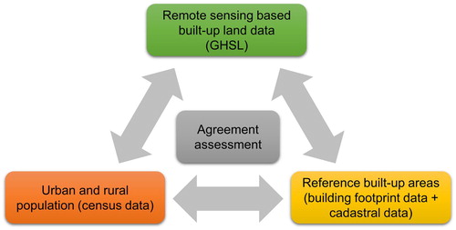
A simple conceptual framework underlies this analysis, as shown in Figure 1. The backbone of the analysis is a series of pairwise comparisons that when combined reveal how remote-sensing based data products describing the built environment, such as GHSL, can be used to understand urban form and the underlying degrees of certainty.

Figure 1. Schematic illustration of the data integration concept used in this work.

2. Data and study area

This study accomplishes two main tasks. First, it evaluates the agreement between different GHSL versions and built-up areas derived from a reference dataset in an accuracy assessment. Second, the same GHSL version is compared to urban depictions derived from census data. Table 1 provides an overview on the basic properties of the datasets used in this analysis. Each data product is briefly described in the following sections.

Table 1. Overview of the datasets and their characteristics used in this study.

Product	Source data	spatial resolution	spatial coverage	temporal resolution	temporal coverage/reference
Reference data	Cadastral parcel data + building footprint data	building footprint level	31 counties within the U.S.	annual	approximately 1870–2016
GHS_LDSMT_2015	Multispectral Landsat data	38 m / 250 m	global	4 discrete epochs	1975–2014
GHS_LDSMT_2017	Multispectral Landsat data	30 m / 250 m	global	4 discrete epochs	1975–2014
GHS_S1	Sentinel-1 Synthetic Aperture Radar data	20 m	global	unitemporal	2015–2017 (reference year 2016)
Urban census blocks	U.S. Census data	census block level	U.S.-wide	decennial	2010

2.1 GHSL data products

2.1.1. GHS built-up grid, derived from Landsat, multi-temporal (1975, 1990, 2000, 2014), release 2016

The first GHSL data package, publically released in 2016, included a global multi-temporal evolution of built-up surfaces derived from Landsat data collections organized in four epochs 1975, 1990, 2000 and 2014 (referred here as GHS_LDSMT_2015) (Pesaresi et al. 2016a). It is the result of processing 32,808 Landsat scenes organized in four data collections, centered at 1975, 1990, 2000 and 2014, as follows:

• 7,588 scenes acquired by the Multispectral Scanner (MS) (collection 1975);

• 7,375 scenes acquired by the Landsat 4–5 Thematic Mapper (TM) (collection 1990);

• 8,756 scenes acquired by the Landsat 7 Enhanced Thematic Mapper Plus (ETM+) (collection 2000); and

• 9,089 scenes acquired by Landsat 8 (collection 2014).

The GHSL method for built-up surface recognition from satellite data was designed for fully automated and reproducible operations. The procedure is based on Symbolic Machine Learning (SML, Pesaresi, Syrris, and Julea 2016b) and uses existing global land cover products as training sets.

The resulting multi-temporal product encodes the presence of built-up surfaces according to the earliest epoch for which the built-up surface presence was detected (i.e. 1975, 1990, 2000, or 2014 epoch) at approximately 38 m resolution (Pesaresi et al. 2016a). According to a quality assessment using detailed cartographic data (Pesaresi et al. 2016a), the accuracy of the GHSL layer was better than the (currently) available global alternatives made by automatic satellite data classification approaches.

2.1.2. GHS built-up grid derived from Sentinel-1 (2016), release 2018 (planned)

Following the successful launch of the Sentinel-1, a proof of concept of the first GHSL experiment exploiting Sentinel-1 data at global scale was performed in 2016 (Corbane et al. 2018), and fully completed in 2017. A dedicated prototype building on the SML classifier was developed for adapting the GHSL production workflow to Sentinel-1 data.

The information extraction of Sentinel-1 data at global scale is described in Corbane et al. (2017). The main workflow builds on SML classifier similarly to the first Landsat derived product (GHS_LDSMT_2015). The SML workflow was adapted to exploit the key features of the Sentinel-1 Ground Range Detected data which are: (i) the spatial resolution of 20 m with a pixel spacing of 10 m and (ii) the availability of dual polarization acquisitions (VV and VH) widely used for monitoring urban areas (see Grey, Luckman, and Holland 2003; Del Frate, Pacifici, and Solimini 2008; Zhu et al. 2012 for some examples) since different polarizations have different sensitivities and different backscattering coefficients for the same target. The learning data at the global level consisted of the union of (i) the built-up layer GHS_LDSMT_2015 obtained from Landsat imagery and (ii) the Global Land Cover map at 30 m resolution (GLC30). The latter one has been also derived from Landsat imagery through operational visual analysis techniques (Chen, Yifang, and Songnian 2014). The massive processing of more than 7,000 Sentinel-1 scenes acquired between 2016 and 2017 was enabled by the Joint Research Centre’s Earth Observation Data and Processing Platform (JEODPP) which is tailored for iterative optimization of big data machine learning methods and fine-tuning of their parameters at full scale (Soille et al. 2018). Notable improvements – in terms of reduction of omission and commission errors – were observed in this new global product derived from Sentinel-1 data (referred here as GHS_S1) in comparison to the Landsat derived built-up areas (i.e. GHS_LDSMT_2015) (Corbane et al. 2017, see also Sabo et al. 2018).

2.1.3. New version of the GHS built-up grid, derived from Landsat, multi-temporal (1975-1990-2000-2014), release 2018 (planned)

The characteristics of the SML classifier allow incremental learning and improvement of the classification outputs as soon as new data depicting built-up areas become available. In other words, the outputs of the SML classifier in one experiment can be used as a training set in the subsequent experiments.

The approach based on incremental learning in the frame of the SML allows for incorporating new, updated learning sets and adjusting what has been learned according to previous examples. This learning method has the advantage of achieving superior efficiency for training minimizing the impact on accuracy. Another beneficial point is that the performance can slightly improve. The results can only get better after each iteration since the level of noise is progressively decreasing with each run of the GHSL workflow, as demonstrated in Pesaresi, Syrris, and Julea (2015).

This characteristic of the SML classifier and the availability of the JEODPP have motivated the design of an experiment aiming to assess the improvement gained by reprocessing the Landsat data collections using the GHS_S1 as a learning set for the SML classifier (Corbane et al. 2017). Therefore, in 2017, the four Landsat data collections were reprocessed following a revised workflow for built-up areas extraction and for the fusion of the four epochs into one multi-temporal product (referred here as GHS_LDSMT_2017). Compared to the procedure used to generate GHS_LDSMT_2015, the revised workflow uses more detailed learning sets on built-up areas and a more consistent global coverage. Besides, incremental learning has been implemented in the SML framework. With this approach, the SML is trained using built-up areas derived from Sentinel-1 (GHS_S1) which in turn were derived from the GHS_LDSMT_2015, leading to a successive refinement and improvement of the results (see Corbane et al., under review for details).

The publicly available version of GHS_LDSMT_2015 (appx. 38 and 250 m spatial resolution grids), and beta-release versions of GHS_LDSMT_2017 (30 and 250 m spatial resolution grids) and GHS_S1 (20 m spatial resolution grid) data, made available to a scientific user community through the Human Planet Initiative (Florczyk et al. 2018), are used in the analysis herein.

2.2. Census data

In this analysis, U.S. census block enumeration units including population counts and block-level urban classification derived from the decennial census 2010 are used. Census blocks represent the smallest spatial units published by the census, delineated by human-made and physical characteristics whose population can vary between zero and a few hundred people (or thousands, in dense urban areas). While typically representing a city block in urban areas, blocks can be large in size in rural areas. There were 11 million blocks reported in the 2010 census. All blocks are classified as either urban or rural. Multiple criteria are used to designate blocks as either urban areas or urban clusters: Urban Areas (UA) are delineated as contiguous sets of blocks demonstrating population density >1,000/mi² and a total population of >50,000. Urban clusters (UC) are contiguous blocks with the same population density criterion (>1,000/mi²), but a total population in the range of 2,500–49,999. Furthermore, blocks in close proximity to an UA or UC (within 2.5 miles) and a population density greater than 500/mi² are classified as urban. Finally, blocks containing industrial and commercial use proximate (within 0.25 miles) to urban blocks in UAs and UCs are included; since 2000, the census has used the National Land Cover Database in order to identify such impervious surface areas (Ratcliffe 2015; and U.S. Census Bureau 2010). While these data are available for the entire U.S. land area, this analysis is subset to blocks in the state of Massachusetts only.

2.3. Reference data

2.3.1. Parcel data

Open cadastral and tax assessment data have become increasingly available to the public – often in GIS-compatible format – for several regions in the U.S. (von Meyer and Jones 2013) and other countries. For this study, we use publicly available parcel data collected from open data sources. Cadastral parcel boundaries are typically of high spatial accuracy since they are acquired using terrestrial or GNSS-based surveying methods, and often include information about structures contained within parcels, such as land use type or the year when structures have been established (Figure 2(a)). Such built-year information allows for the creation of multi-temporal cross-sections of parceled land at high spatial and annual temporal resolution and, thus, constitute a valuable data source for modeling areas of residential development (Leyk et al. 2014) or population estimates for small areas (Tapp 2010) and at different points in time (Zoraghein et al. 2016; Zoraghein and Leyk 2018). Common challenges include limited data accessibility impeded by restrictive data policies in many regions, large data volumes requiring computationally intense efforts (Manson et al. 2009) and inconsistent data modeling across different regions. Moreover, considerable variations in parcel size impede the analysis and need to be taken into account, especially across the urban-rural continuum (Leyk et al. 2013).

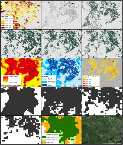
Figure 2. Datasets used in this study shown for Northampton (Massachusetts), USA: (a) Parcel data including built-year information, (b) building footprint data, (c) rasterized reference built-up presence-absence surface in 2015, GHSL built-up areas (d) GHS_LDSMT_2015, (e) GHS_LDSMT_2017, (f) GHS_S1, (g) reference built-up density surface in 2015, (h) derived development intensity strata with white pixels indicating unreliable reference data, (i) per-pixel built-up proportions derived from the reference data in 2015, (j) urban census blocks, GHS_LDSMT_2015 250 m derived urban masks for a binarization threshold of (k) 1%, (l) 25%, (m) 50%, (n) agreement categories from overlaying GHS_LDSMT_2015 250 m 1% urban mask and urban census tracts, and (o) a high resolution aerial image (Source: ESRI) of the shown extent.

2.3.2. Building data

Building footprint data are traditionally derived from airborne surveying measurements or aerial image interpretation. However, recent developments in deep learning based information extraction methods from geospatial earth observation data (i.e. aerial or satellite-based multispectral imagery at high and very high spatial resolutions) and large-scale LiDAR mapping constitute a promising alternative to the traditional methods holding the potential for accurate acquisition of building footprint data at high spatial resolution and at large spatial extents (e.g. Sugarbaker et al. 2014; Facebook and CIESIN 2016; Yuan 2016). With these increasing efforts in detecting and mapping existing structures, building footprint data are becoming increasingly available as open data, which we use in this study to spatially refine the snapshots of built-up parceled land. This refinement is especially effective in rural areas where parcel units can have large areal extents and are expected to drastically overestimate built-up land if they remain unrefined. For some administrative regions in the U.S. (31 counties) in which parcel data including temporal information are available, we used building data (Figure 2(b)) that allowed us to create a large validation database which can be used to quantify the accuracy of built-up land layers in different regions of the U.S. (Uhl et al. 2016) and thus under different landscape conditions, vegetation types, settlement histories, etc., and for different points in time. In addition to that, this database has successfully been employed for further information extraction applications in the fields of remote sensing (Uhl and Leyk 2017) and map processing (Uhl et al. 2017).

2.4. Study areas

The selection of the study areas is driven by the spatial coverage of the reference database which covers 31 counties (i.e. an area of >45,000 km² and more than 6 million parcel objects, see Appendix and Leyk et al. 2018) across the U.S. and includes the state of Massachusetts, USA. Whereas the GHSL accuracy assessment is conducted within all 31 counties, the agreement analysis between GHSL-derived urban land and census data is limited to the state of Massachusetts only. A final cross-comparative agreement analysis compares the reference data with urban blocks from the U.S. census (described below) also for the state of Massachusetts. We do an in-depth analysis of Massachusetts only, owing to data constraints, but aim to draw some conclusions more broadly and connect the results to other research underway that is international in scope.

3. Methods

Drawing our methods largely from another study that examines GHS_LDSMT_2015 across multiple time points and locations (Leyk et al. 2018), in this study we examine that dataset but only for the most recent time point, and compare it with the newer versions (one of which is only available for a single time point, 2016).

3.1. GHSL data product evaluation within U.S. Counties

First, we assess the agreement between each of the three GHSL products and the built-up areas derived from the reference database. Following an earlier approach (Leyk et al. 2018) this assessment results in accuracy statistics to evaluate the different GHSL data products for different regions across varying development intensities that represent a continuum of urban, peri-urban and rural settings for one point in time (i.e. approximately 2015).

3.1.1. Creating validation data

The integration of cadastral parcel and building objects, both collected from heterogeneous data sources in 2016, is realized through mutual spatial joining, allowing for the identification of building objects within each parcel area in order to transfer the built year and land use information from the parcel to the building object. Establishing mutual spatial relationships (i.e. buildings within parcel, parcel, containing building) makes it possible to identify discrepancies between parcel and building data (i.e. parcels without built-year information but containing buildings, and parcels holding a valid built year attribute, but not containing any building objects). Areas of such discrepant information (i.e. approximately 15% of the total study area) are excluded from the study, in order to minimize uncertainty in the reference data. The integrated data product is then rasterized into grid cells of 2 m, as a base for further processing, while preserving a sufficiently high level of spatial granularity.

3.1.2. Creating the reference surfaces and resampling test data products

Agreement assessment is conducted by using pixel-based map comparison techniques. The reference data is converted into binary raster layers indicating the presence or absence of built-up areas (Figure 2(c)). The abstract class ‘built-up area’ applied to the GHSL (Pesaresi et al. 2013) in practice translates to any grid cell that overlaps with a built-up and roofed structure. In compliance with this definition, we converted the rasterized, integrated reference data (2 m spatial resolution) to a raster surface compatible to GHS_S1 (originally in WGS84 Web Mercator projection, EPSG:3857, reprojected to Albers equal area conic projection for the contiguous U.S., EPSG:102003 using nearest-neighbor resampling). This compatibility includes spatial compatibility (i.e. spatial resolution of approximately 20 m, identical grid cell position and orientation), temporal compatibility (i.e. using the same temporal reference year), and semantic compatibility (i.e. using the same definition of the abstract built-up land class). In the same way, the other GHSL datasets are reprojected from their native projections into EPSG:102003 and upsampled to the GHS_S1 resolution using nearest-neighbor resampling to ensure compatibility between all layers given the fine resolution of the GHS_S1 data (Figure 2(d–f)).

In addition to this reference built-up presence-absence surface, we derived built-up density surfaces based on the reference data, using a 200 m focal window as a proxy variable for localized development intensity and applying a point density function (Figure 2(g)). Based on this continuous built-up density surface, thresholds are applied to generate spatial strata of development intensity that could be loosely related to urban, peri-urban, and rural areas. Therefore, thresholds from Leyk et al. (2018) (i.e. built-up density <0.5%: rural stratum, 0.5%–5%: peri-urban stratum, and >5% urban stratum) are applied (Figure 2(h)). Furthermore, the fine-grained reference data (at 2 m spatial resolution and created in EPSG:102003) is used to derive a coarser resolution (i.e. 20 m) raster surface indicating per-pixel proportions of built-up areas (Figure 2(i)). Both per-pixel built-up proportions and built-up density surfaces are spatially compatible to the previously described reference and test surfaces and are used to study their variability within classes of agreement / disagreement between the different GHSL products as well as between census urban/rural depictions and GHSL-derived urban areas.

3.1.3. Computing accuracy measures for different development intensities and cross-product comparison

Each of the different GHSL data layers is compared pixel-wise to the reference data and confusion matrices are created to derive various accuracy measures (Fielding and Bell 1997; Nguyen, Bouzerdoum, and Phung 2009) overall and for the different strata of development intensity across the 31 counties. The following accuracy measures have been computed:

• Percentage correctly classified (PCC, also known as Overall Agreement): PCC is commonly used to evaluate classification performance, but tends to be inflated if imbalanced class proportions are involved (Rosenfield and Melley 1980). Nevertheless, this measure is reported, since it is commonly used in the literature, and thus allowing the reader to easily relate the results presented herein to other works.

• Kappa Coefficient of Agreement (Kappa) (Cohen 1960), accounting for agreement by chance between the compared class labels.

• G-Mean: The geometric mean of User’s and Producer’s accuracy (Fawcett 2006) characterizing commission and omission errors of the labels of interest in an integrated manner invariant to inflation effects due to imbalanced class proportions, and suitable for non-normalized data.

• F-Measure: Harmonic mean of sensitivity and specificity (Kubat and Matwin 1997) accounting for the accuracy of both the positive and negative classes.

• User’s and Producer’s Accuracies (Fielding and Bell 1997) corresponding to the errors of commission and omission, respectively. We report these measures in addition to G-mean which potentially occludes extreme commission or omission errors.

• Quantity disagreement and allocation disagreement, as proposed by Pontius and Millones (2011), allowing for separating the observed disagreement between test and reference data into components corresponding to thematic and positional disagreement.

These accuracy measures illuminate the agreement between reference and test data from different point of views and allow for an assessment of the different GHSL versions. F-Measure and G-Mean tend to be less inflated in the case of imbalanced class proportions as compared to PCC. As shown in earlier work (Leyk et al. 2018), the detection rate of individual structures in remote, isolated locations is very low in the GHSL data. Therefore, the study areas are stratified in similar ways based on the level of built-up density, as described before, and in each of these strata the accuracy assessment is carried out, separately (see Olofsson et al. 2013). For each GHSL data product and each stratum, a confusion matrix is generated and accuracy measures are computed for each of these strata across all 31 counties.

In addition to that, we visualize the agreement-disagreement proportions of pixels from the reference data and the built-up land labels for each of the three GHSL data products to better understand the mutual degrees of agreement between them and to identify potential systematic effects. Furthermore, for the different cases of cross-product (dis)agreement, we analyze the statistical distribution of built-up density and per-pixel built-up proportions by using boxplots. This will facilitate some diagnostic work elucidating how the different GHSL data layers are performing, and what weaknesses and strengths can be observed for each of them.

3.1.4. Regression analysis to evaluate statistical relationships between GHSL and reference data

To complete the series of assessment steps outlined in Leyk et al. (2018), we conduct a linear regression analysis to examine quantity agreement of built-up areas derived from the GHSL data products as compared to the reference data at different spatial aggregation levels. We run these models using spatially aggregated built-up land proportions, approximating to the aggregated 250 m GHSL products (i.e. proportions of built-up areas within blocks of 250 × 250 m) used for the agreement assessment of GHSL and census-derived urban population, described below.

These linear regression models are calculated for each GHSL data product and each built-up density stratum across the 31 test counties. As shown in our recent research, this regression will help to: (1) mitigate potential spatial misalignment issues and to separate between thematic and positional uncertainty; (2) provide a robust statistical framework to estimate this relationship across different built-up density strata; and (3) provide a basis to quantify systematic bias and derive parameters that could be typical for the density stratum considered or the sensor or extraction method applied. Thus, the results could potentially be useful for applying the GHSL in other regions to compensate for uncertainty or underestimation / overestimation effects.

3.2. Informing urban classification through built-up land data

In the second part of this contribution, we assessed the agreement (a) between population-based urban classifications derived from U.S. census data (i.e. at census block level) and built-up areas derived from the reference database (Section 3.2.1), and, in comparison to that (b) between the census-based urban areas and urban masks derived from spatially aggregated GHSL products, i.e. GHS_LDSMT_2015 and GHS_LDSMT_2017 at a spatial resolution of 250 m (Section 3.2.2).

3.2.1. Understanding official census classes with respect to the reference data

Based on U.S. census blocks, which are classified as urban or not urban by the U.S. Census Bureau, population-based masks of urban and non-urban areas are derived. We rasterize the resulting urban masks to a spatial resolution of 20 m to generate a raster surface compatible to the reference built-up presence–absence surface (see Figure 2(j) for an example). These two surfaces are input to a pixel-wise map comparison to calculate confusion matrices for each county in the state of Massachusetts. Based on these matrices, we were able to carry out a quantitative assessment of agreement between census-based urban areas and parcel-based delineations of built-up areas, respectively. Agreement measures are reported and visually analysed at the county-level to assess regionally dependent variations in the degree and nature of agreement.

3.2.2. Assessing spatial agreement between GHSL-derived built-up masks and census data urban designations

Similarly to a spatial approach proposed by Dorélien, Balk, and Todd (2013) and refined for census units by Balk et al. (2018), the agreement between GHSL-derived built-up areas and urban census blocks is assessed. For this agreement assessment, we use the spatially aggregated versions of GHS_LDSMT_2015 and GHS_LDSMT_2017 at a spatial resolution of 250 m. These data products are continuous raster surfaces representing the per-pixel percentage of built-up area. Several thresholds (i.e. 1%, 25%, 50%) are applied in order to create binary built-up presence–absence layers that are compared to the census-based urban masks. These aggregated versions of GHSL are provided originally in World Mollweide projection, EPSG:54009, and were reprojected to Albers equal area conic projection for the contiguous U.S., EPSG:102003 using nearest-neighbor resampling. Since the choice of these thresholds is expected to heavily influence the results of the comparison, this analysis will help data users to estimate the effects associated with such thresholding methods (see Section 4.4). Some examples of built-up masks derived from GHS_LDSMT_2015 are shown for these three thresholds in Figure 2(k–m). The built-up masks resulting from combining each of the two source data products with each of the three binarization thresholds are vectorized and overlaid with the census block polygons classified as urban. Based on this overlay four categories of agreement are created (Balk et al., 2018): Areas of urban agreement where the census urban definition and GHSL threshold are both met; areas classified as census urban only as the census designates the block as urban but the GHSL built-up threshold is not met; areas classified as built-up by GHSL only as the GHSL built-up threshold is met, but the census classifies such blocks as rural; and finally, census rural only as these are areas designated by the census as rural and they do not meet the threshold of GHSL (Elsewhere we call these classes: Urban agreement (UAg), Built-up land only (BULO), Urban people only (UPO) and rural extents (RE); see Balk et al., 2018). These are shown in Figure 2(n), exemplarily, for the GHS_LDSMT_2015 250 m version derived built-up mask using a binarization threshold of 1%.

We compare the areas associated with each category and allocate population counts to each category using proportional areal weighting. Using these statistics, we quantify the agreement between these two data products within the state of Massachusetts related to population and area. Furthermore, for each urban / built-up agreement category derived from the various overlays based on the different data product-threshold combinations we assess the statistical distribution of development intensity (computed based on the reference built-up density surfaces) using boxplots. Such a visualization will help to identify the levels of development intensity at which agreement or disagreement of land designated as urban and built-up land occurs.

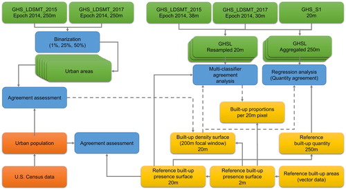
Figure 3 provides an overview of the workflow for the agreement assessment between GHSL-derived built-up land masks, parcel-based reference data and urban/rural extents obtained from census data.

Figure 3. Workflow of the data processing and agreement assessments conducted in this work.

4. Results

4.1. GHSL accuracy assessment and cross-comparison

The pixel-wise map comparison of GHS_LDSMT_2015, GHS_LDSMT_2017, and GHS_S1 against the reference built-up presence–absence surface was conducted separately for each development intensity stratum and reported over all 31 validation counties. Whereas most accuracy measures shown in Figure 4 indicate for each GHSL product a positive trend from the rural to the urban stratum, PCC shows an opposite trend. This measure is known for being sensitive to imbalanced class distributions and tends to inflate in such cases, which explains the high magnitude in the rural stratum, where the degree of imbalance is high due to the high proportion of not built-up land. Interestingly, the GHS_S1 product achieves consistently slightly lower accuracy in the urban stratum, as compared to the two Landsat-based GHSL products. Possible reasons are the higher spatial resolution (i.e. 20 m) causing a higher sensitivity to positional offsets, as compared to the Landsat-based versions, where this effect is mitigated through the use of larger grid cells (38 and 30 m, respectively). On the other hand, in the peri-urban stratum, GHS_S1 shows higher Producer’s Accuracy than the other two GHSL products, indicating a higher degree of correctly detected built-up areas. Considering the class-independent accuracy measures (i.e. Kappa, F-Score, G-Mean), the GHS_LDSMT_2017 product outperforms the two other products in all three strata.

Figure 4. Results of the accuracy assessment of the three GHSL versions for rural, peri-urban, and urban strata across 31 counties. (a) Kappa index, (b) PCC, (c) User’s Accuracy, (d) Producer’s Accuracy, (e) F-measure, (f) G-mean, (g) quantity disagreement, and (h) allocation disagreement.

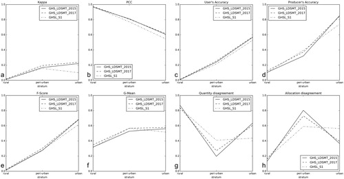
Quantity and allocation disagreement separates overall disagreement into two components describing thematic and positional uncertainty. Here, GHS_S1 shows a significantly different trend than the other GHSL products. Whereas in the rural stratum, all three GHSL products show high quantity disagreement (i.e. underestimating the amount of built-up land), GHS_S1 better estimates built-up quantity in the urban stratum (less overestimation due to higher spatial resolution). Positional offsets affecting GHS_S1 stronger than the Landsat-based products result in an increased allocation disagreement in the urban stratum.

Besides comparing the three GHSL products to the reference data, we visually assessed agreement between themselves by encoding agreement among all products at each pixel location using a binary vector of dimension 4 × 1. These binary vectors are color-encoded and plotted as columns, sorted numerically (e.g. [0,0,0,0],[0,0,0,1],[0,0,1,1], … ,[1,1,1,1], where each position corresponds to one product, and 1/0 indicate agreement or disagreement of the respective labels, i.e., 0 = not built-up, 1 = built-up, see Figure 5(a)) and sorted according to the built-up density derived from the reference data at each respective pixel location in a non-linear scale (Figure 5(b)), both for a random subset (N = 200,000) of the evaluated pixels across all study areas.

Figure 5. Agreement between the three GHSL versions in a random sample of 200,000 pixels across the 31 counties (a) sorted by agreement combination, and (b) sorted by built-up density.

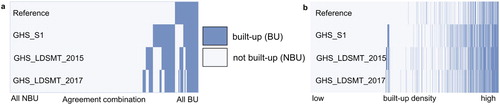
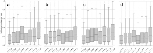
Figure 5(a) graphically depicts the amount of false positives (dark blue where reference shows light blue) and false negatives (light blue where reference shows dark blue) of all product assessments in comparison with the reference. It can be seen that GHS_LDSMT_2015 correctly classifies a considerable amount of what has been false positives for the GHS_S1, on the one hand, but producing other false positives at pixel locations where GHS_S1 correctly predicts not built-up land. These deviations are likely caused by the increased spatial aggregation. A higher level of agreement can be observed between GHS_LDSMT_2015 and GHS_LDSMT_2017, resulting in thinner complementary light blue and dark blue columns. Figure 5(b) shows the agreement between the three GHSL products across the continuum of built-up densities. This visualization reveals a high level of agreement between the three products at locations of very high built-up density, and indicates that GHS_S1 has a stronger tendency to classify a pixel as built-up in regions of lower built-up density as compared to the two other GHSL products. In addition to that, all three GHSL versions seem to falsely detect built-up land at very low levels of built-up density, likely caused by impervious surfaces (e.g. roads) in rural areas that are classified as built-up. Besides assessing the agreement between the three GHSL products across the continuum of built-up densities, we assessed the statistical distribution of built-up density stratified by agreement categories (Figure 6). These boxplots indicate high average built-up density at locations where all GHSL products correctly predict built-up land (1,1,1,1) over all study areas (Figure 6(a)). At locations where GHS_LDSMT_2015 and GHS_LDSMT_2017 correctly classify built-up land (1,0,1,1), we observe slightly lower values of average built-up density, and less dispersion. Another peak of built-up densities can be observed at locations where all three GHSL versions falsely detect built-up land (0,1,1,1), likely caused by misclassified pixels containing impervious but not built-up surfaces (e.g. parking lots, roads) ín areas of high development intensity. Low levels of built-up density at locations where only GHS_S1 correctly detects built-up areas (1,1,0,0) indicate that this combination tends to occur in rural areas, indicating higher sensitivity for built-up environments in these problematic settings. These patterns can be observed in similar ways for individual counties of highly urban character (New York City, Figure 6(b)), in peri-urban areas (Ramsey County, Minnesota, Figure 6(c)), and in mostly rural regions (Boulder County, Colorado, Figure 6(d)). Similarly, we visualize the distributions of per-pixel built-up proportions for classes of agreement between the GHSL versions (Figure 7). These plots indicate how mixed-pixel effects in the multi-spectral remote sensing data underlying the GHSL products affect the classification results. For example, pixels of close to 100% built-up proportion (i.e. large structures) are mostly correctly detected as built-up by all GHSL versions (1,1,1,1). The built-up proportions in pixels only correctly detected by GHS_S1 are of considerably lower average built-up proportions which reflects the higher spatial resolution and thus higher sensitivity of the underlying Sentinel data. As expected, pixels that only contain very small built-up proportions are not detected as built-up by any of the GHSL products. It should be noted that resampling effects and positional offsets in the reference data (i.e. building footprint data) may interfere.

Figure 6. Distribution of built-up density by agreement combination for (a) all 31 counties, (b) New York City (urban), (c) Ramsey County (MN, peri-urban), and (d) Boulder County (CO, peri-urban / rural).

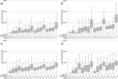
Figure 7. Distribution of reference built-up proportion per pixel for different agreement combinations (reference positives only) in (a) New York City, (b) in Ramsey County (MN), (c) in Boulder County (CO), and (d) over all 31 counties.

4.2. Built-up quantity regression analysis

We established statistical relationships between built-up quantity estimated by the three GHSL versions and the reference built-up quantity in blocks of 250 × 250 m, overall and separately for each development intensity stratum across all 31 counties. Figure 8 shows regression plots for each configuration, here visualized for a random subset of 5% of the total count of blocks. Table 2 shows the numerical regression results. Several trends can be observed: (A) The explanatory power of GHSL-based built-up quantity increases from rural towards urban strata, which manifests in increasing R-squared values. Increasing slopes from 0.03 in rural strata to 0.6 in urban strata additionally support this observation. This effect can be observed for all three GHSL products. (B) In the urban stratum, slope values increase with increasingly coarser spatial resolution of the GHSL product. This is a result of an observed overestimation of built-up land in urban areas when using fine-resolution data, e.g. by falsely detecting impervious surfaces as built-up areas. This effect is strongest in GHS_S1 and leveraged with coarser spatial resolution of the GHSL product. (C) The magnitude of the intercepts in the peri-urban and urban strata also seems to be related to the spatial resolution of the GHSL product, with highest intercepts for the GHS_LDSMT_2015 product (38 m spatial resolution), revealing a tendential underestimation of built-up quantity in blocks of low reference built-up proportion. (D) Additionally, the point patterns in the scatterplots reveal further details. For example, in the peri-urban stratum, the two Landsat-based GHSL versions tend to underestimate built-up quantity, as opposed to GHS_S1, which shows a higher number of blocks where built-up proportion is overestimated.

Figure 8. Results of the regression analysis predicting reference built-up quantity in blocks of 250 m across different strata of development intensity and over all strata (left to right) based on GHS_S1, GHS_LDSMT_2017, and GHS_LDSMT_2015 (thus sorted by increasing spatial resolution from top to bottom).

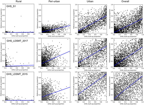
Table 2. Numerical regression results.

Product	Stratum	Slope	Intercept	R-squared
GHS_S1	rural	0.03	0.01	0.04
GHS_S1	peri-urban	0.45	0.08	0.54
GHS_S1	urban	0.55	0.08	0.71
GHS_S1	overall	0.5	0.03	0.76
GHS_LDSMT_2015	rural	0.01	0.02	0.01
GHS_LDSMT_2015	peri-urban	0.38	0.14	0.28
GHS_LDSMT_2015	urban	0.6	0.18	0.65
GHS_LDSMT_2015	overall	0.69	0.06	0.75
GHS_LDSMT_2017	rural	0.02	0.01	0.03
GHS_LDSMT_2017	peri-urban	0.41	0.11	0.35
GHS_LDSMT_2017	urban	0.6	0.14	0.65
GHS_LDSMT_2017	overall	0.67	0.04	0.78

4.3. Comparing urban areas derived from census and parcel data

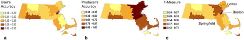
We assessed the agreement between urban census blocks and reference data derived from parcel data and report agreement measures for all counties of the state of Massachusetts, visualized in quintile classes (Figure 9). This assessment provides a baseline that helps forming expectations for the overlay of GHSL-based data with census data and understanding of the potential outcome across different settings along the urban-rural continuum. The different measures can be linked to the different urban classes that will be built in the next section. For example, in regions where higher F-measures can be found it can be expected that there are larger proportions of urban agreement – areas where the census definition and GHSL (at a given threshold) agree. Indeed, it can be seen in Figure 9(c) that highest agreement between census and reference data occurs in counties containing larger urban agglomerations (i.e. Boston, Springfield, Lowell), low agreement was observed in counties of mostly rural character. Furthermore, low User’s accuracy (Figure 9(a)) indicate higher commission errors and thus higher proportions of Census Urban Only could be expected. Similarly, low Producer’s accuracy (Figure 9(b)) refers to higher omission errors and thus possibly high GHSL Only proportions. These links provide a more objective idea of what we can expect to identify in the GHSL-census overlay experiments reported in the following section.

Figure 9: Agreement measures between urban areas derived from parcel and census data: (a) User’s Accuracy, (b) Producer’s accuracy, and (c) F-Measure.

4.4. Agreement assessment between GHSL and census data

The results of the agreement assessment for urban areas derived from binarizing GHS_LDSMT_2015 and GHS_LDSMT_2017 250 m aggregates using different built-up thresholds (50%, 25%, and 1%) are shown in Table 3 and Figure 10. We observe that for the 1% and 25% binarization thresholds the area proportions of urban agreement increase when employing GHS_LDSMT_2017, whereas the opposite trend can be observed for the 50% binarization threshold, indicating that a less conservative separation criterion needs to be applied to generate urban areas from GHS_LDSMT_2017 in agreement with urban populations. Similarly, in areas classified by the census as urban, but which do not meet the respective GHSL thresholds, a greater proportion of people are capture by GHS_LDSMT_2017 than by GHS_LDSMT_2015 at the 50% threshold, but the inverse is found at the more inclusive thresholds of 25% and 1% built-up. Though the fractions are very small, more population and land is found in areas that are detected by GHS_LDSMT_2017 than by GHS_LDSMT_2015 but not designated as urban by the census, at the more inclusive thresholds (25% and 1% built-up). Note that in Table 3, proportions of the urban agreement, census urban only, and GHSL only categories are referred to the Urban Inclusive, comprising these three categories. This allows for assessing the area proportions independenly from the dominating census rural only category.

Figure 10. Agreement categories for urban census blocks and GHS_LDSMT_2015 using binarization thresholds of (a) 1%, (b) 25%, (c) 50% and (d-f) for GHS_LDSMT_2017, respectively.

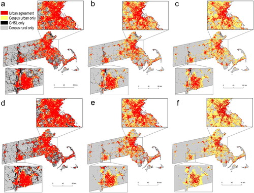
Table 3. Area and allocated population values in the agreement categories for the overlay of census and GHSL-derived urban areas.

		Count and Percentage, 50% Built-up				Count and Percentage, 25% Built-up				Count and Percentage, 1% Built-up
		GHS_LDSMT 2015		GHS_LDSMT 2017		GHS_LDSMT 2015		GHS_LDSMT 2017		GHS_LDSMT 2015		GHS_LDSMT 2017
		Count	%	Count	%	Count	%	Count	%	Count	%	Count	%
Population	Urban Inclusive	6,058,223	92.53	6,058,281	92.53	6,090,106	93.01	6,100,635	93.17	6,216,655	94.95	6,256,290	95.55
	- Urban Agreement	4,142,377	68.38	4,062,046	67.05	4,802,149	78.85	4,942,501	81.02	5,605,079	90.16	5,776,605	92.33
	- Census urban only	1,890,699	31.21	1,977,354	32.64	1,229,289	20.19	1,096,498	17.97	427,773	6.88	262,820	4.20
	- GHSL only	25,147	0.42	18,881	0.31	58,668	0.96	61,635	1.01	183,803	2.96	216,865	3.47
	Census rural only	489,406	7.47	489,348	7.47	457,523	6.99	446,994	6.83	330,974	5.05	291,339	4.45
Area (km^2)	Urban Inclusive	8,408	40.05	8,295	39.52	8,810	41.97	8,776	41.80	10,623	50.60	10,891	51.88
	- Urban Agreement	2,637	31.36	2,452	29.56	3,853	43.73	4,086	46.56	6,023	56.70	6,621	60.79
	- Census urban only	5,457	64.90	5,654	68.15	4,236	48.08	4,017	45.77	2,067	19.46	1,482	13.60
	- GHSL only	314	3.73	190	2.29	721	8.19	673	7.67	2,533	23.84	2,789	25.60
	Census rural only	12,585	59.95	12,698	60.48	12,183	58.03	12,217	58.20	10,370	49.40	10,102	48.12
Population Density (persons/km^2)	Urban Inclusive	721		730		691		695		585		574
	- Urban Agreement	1,571		1,657		1,246		1,209		931		872
	- Census urban only	346		350		290		273		207		177
	- GHSL only	80		100		81		92		73		78
	Census rural only	39		39		38		37		32		29

More inclusive thresholds result in lower population densities in areas of urban agreement and census urban only but higher ones in built-up land areas only with GHS_LDSMT_2017 as opposed to GHS_LDSMT_2015, consistent with the above findings. Even though population densities in the U.S. are much lower than found elsewhere, the sensitivity of those density levels to the GHSL threshold may be significant for downstream usages of these combined data. In general, the improvements to GHSL brought about by including Sentinel-derived built-up areas into the information extraction process result in slightly less agreement when a conservative built-up threshold (50%) is used but more agreement at more inclusive thresholds, consistent with the improved spatial resolution and detection capabilities of the Sentinel-1 sensor, and as found in the regression results above.

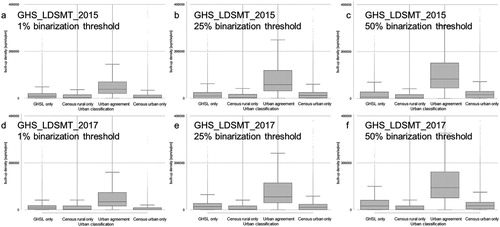
It is worth noting that the particular thresholds used here are themselves arbitrary but that they reveal levels of built-up densities that could be used to model urbanization (or changes in it) where detailed census data are lacking. Given that at the most inclusive threshold (1%) 92% of all urban population is captured suggests such potential. The improvements brought about by Sentinel-1 increase GHSL’s ability to capture areas of agreement of urban land by 4 percentage points (also see reduction by 6 percentage points of land classified as census urban only) but these areas remain those that will likely require more nuanced criteria and modeling of GHSL (such as nuanced contiguity rules, mimicking those used in the census itself) to be captured fully. Figure 10 shows the four agreement categories for GHS_LDSMT_2015 and GHS_LDSMT_2017 for the thresholds of 1%, 25%, and 50%, respectively. In addition to that, we assess the level of development intensity for the different urban classes created through the overlay of GHSL-derived built-up masks and urban census blocks (Figure 11). Here, both GHS_LDSMT_2015 and GHS_LDSMT_2017 show a clear trend of increasing built-up density in areas of urban agreement with increasing binarization threshold applied. This reflects the strong positive correlation between aggregated GHSL built-up proportion and built-up density computed within focal windows as reported above.

Figure 11. Distribution of built-up density for categories of agreement between census-derived urban population and built-up land derived from GHS_LDSMT_2015 (top row) and GHS_LDSMT_2017 (bottom row) based on binarization thresholds of 1%, 25%, and 50% (from left to right).

5. Discussion

In this work, we presented a cross-comparison between remote sensing, cadastral, and population census based datasets modeling the urban continuum. In a first part, we assessed the agreement between highly accurate reference data based on parcel and building footprint data and various versions of the GHSL. Previous findings concerning the accuracy of remote sensing derived built-up land layers across the rural-urban continuum could be confirmed, while some important differences due to changes in underlying sensors were identified. The addition of Sentinel-1 based data resulted in higher sensitivities in peri-urban and rural settings, thus overcoming some of the limitations from the first version of GHSL without including information extracted from Sentinel-1 data, however, this sensitivity often resulted in lower accuracy measures due to falsely detected impervious land entities. The cross-comparison of different GHSL versions revealed great potential in that the strengths of different data products might be combined in future research efforts to improve the classification accuracy in rural settings, significantly.

Furthermore, the ability of remote sensing derived built-up land data to model urban populations was examined, with the conclusion that the combination of Landsat and Sentinel-1 data for the creation of the GHSL improves the agreement to census-derived urban populations, especially when more inclusive thresholds are used to binarize the continuous GHSL built-up land surfaces. However, future work will be necessary to establish effective and generalizable thresholding criteria allowing for the delineation of urban land based on remote sensing derived built-up land data. It should be noted that part of the detected disagreement between GHSL-derived urban masks and census-based urban definitions is due to the definition of urban census blocks in the U.S. census and the fundamentally different abstract class of built-up land used in the GHSL concept. In addition to that, we evaluated how parcel-based reference data agrees with urban populations, showing satisfactory levels of agreement in areas of urban and peri-urban character only.

It is worth noting that the conducted analyses are potentially affected by three types of temporal discrepancies: (a) Different data acquisition dates of the recent epochs of GHSL versions (i.e. 2014 for GHS_LDSMT_2015 and GHS_LDSMT_2017, and 2016–2017 for GHS_S1, respectively), (b) variation in the most recent revision date of the cadastral reference data between counties that were collected from different sources in 2016, and (c) temporal offset between census data referenced to 2010, the various GHSL versions and the reference data. The effects of temporal discrepancies between the different versions of GHSL and the reference data (i.e. a range of approximately 2 years) on the conducted comparative analyses can be neglected given the typical pace of urban growth, the duration of construction phases, and thus, the inherent uncertainty in temporal references of built-up areas. The temporal offset between census data and the other data used in this study is of greater magnitude (i.e. 4–6 years) and may affect the results of the analyses involving census data. However, this effect is assumed to be of systematic nature and thus only minor effects are expected in Section 4.3, and across different GHSL threshold levels (Section 4.4).

Besides these temporal discrepancies, the presented results may be affected by additional uncertainty introduced during the reprojection and resampling of the data used in this study, which is inevitable for the cross-comparison of multi-source data as presented herein. Additional positional uncertainty due to transformations between cartographic projections is kept to a minimum by using adequate, region-specific transformation parameters. However, in the case of raster data reprojection, the applied resampling technique (i.e. transferring binary or continuous pixel values from source to target grids) may slightly modify the data and thus, affect subsequent analysis results. This also applies to the upsampling of GHSL data to the target resolution used for the pixel-wise agreement assessment (i.e. 20 m), and to the downsampling (i.e. aggregation) of GHSL data to the spatial resolution of 250 m used for the regression analysis, especially in cases where the original cell sizes (i.e. 30, 38 m) do not nest in grid cells of 250 m. These resampling steps may cause small, randomly distributed spatial offsets in the data. However, since the presented results are based on large amounts of individual grid cells and aggregated across multiple, spatially disjunct study areas, these effects can be considered negligible for the interpretation of the results presented herein.

The availability of cadastral data is relatively rare, and thus here we employed a two-pronged strategy that allowed to place the comparison of cadastral data with GHSL variants to those of census data with GHSL variants, in order to be able to contextualize the comparison of GHSL with census data in the absence of such parcel data. Future work will include the systematic derivation of sensitive thresholds to model urban populations based on GHSL data under different geographical conditions, by expanding the study areas to other countries such as India or Mexico or other localities that can be characterized by a similar level of census data richness, but fundamentally different population and urbanization dynamics. Such analyses will reveal the generalizability of findings made on the basis of data available in the U.S., and will allow to establish guidelines for data users at a more global level, holding the potential to develop predictive models for selected agreement measures to be applied to regions of the world, where data is sparse. Such an approach could help to create improved models to allocate human populations in regions where remote sensing derived built-up land data are the only available data source at high spatial resolution or be used simply as a proxy for urban settings where such urban footprints are otherwise lacking.

Acknowledgments

The content is solely the responsibility of the authors and does not necessarily represent the official views of the National Institutes of Health. We thank Hasim Engin for research assistance.

Disclosure statement

No potential conflict of interest was reported by the authors.

ORCID

Johannes H. Uhl http://orcid.org/0000-0002-4861-5915

Stefan Leyk http://orcid.org/0000-0001-9180-4853

Deborah Balk http://orcid.org/0000-0002-9028-7898

Christina Corbane http://orcid.org/0000-0002-2670-1302

Additional information

Funding

This research has been funded, in part, by the U.S. National Science Foundation (Directorate for Social, Behavioral and Economic Sciences) award #1416860 to the City University of New York, the Population Council, the National Center for Atmospheric Research and the University of Colorado at Boulder. It has been supported, in part, by the Eunice Kennedy Shriver National Institute of Child Health and Human Development of the National Institutes of Health under Award Number P2CHD066613. Furthermore, this work has been funded, in part, by an Andrew Carnegie Fellowship (#G-F-16-53680) from the Carnegie Corporation of New York to D. Balk. Innovative Seed Grant funding from the University of Colorado, support through Earth Lab, a University of Colorado Boulder Grand Challenge Initiative, as well as a development grant received from the University of Colorado Population Center (CUPC) at the Institute of Behavioral Science (University of Colorado Boulder), are acknowledged.

Appendix

The 31 counties used for validation in this work.

Table

County	State	Population 2015	Area [sqkm]	% built-up according to reference data
Anoka County	Minnesota	341742	1153.1	10.3
Baltimore County	Maryland	827794	1623.9	12.6
Barnstable County	Massachusetts	214665	1177.8	12.3
Benton County	Oregon	86414	1747	0.9
Berkshire County	Massachusetts	128565	2451	2.6
Boulder County	Colorado	313864	1780.4	3.3
Bristol County	Massachusetts	554626	1529.6	11.4
Carver County	Minnesota	97396	970	4.2
Dakota County	Minnesota	412182	1522.3	7.8
Dukes County	Massachusetts	17320	319.5	4.6
Essex County	Massachusetts	770486	1388	12.2
Franklin County	Massachusetts	70927	1876.8	1.9
Hampden County	Massachusetts	469566	1641.9	8.3
Hampshire County	Massachusetts	161106	1413.5	4.1
Hennepin County	Minnesota	1212097	1566.4	20.8
Hillsborough County	Florida	1318325	2800.3	13.4
Manatee County	Florida	351771	2064.4	6.5
Mecklenburg County	North Carolina	1011928	1409.6	23.8
Middlesex County	Massachusetts	1572523	2196.6	16.7
Milwaukee County	Wisconsin	957913	249.1	34
Monmouth County	New Jersey	629018	1255.9	15.5
Nantucket County	Massachusetts	10821	155.5	6.5
New York City	New York	8537673	781.1	54.3
Norfolk County	Massachusetts	692688	1083.9	16.5
Plymouth County	Massachusetts	507050	1822.3	9.3
Ramsey County	Minnesota	533634	439.5	30.8
Sarasota County	Florida	397024	1569.5	11.2
Suffolk County	Massachusetts	769809	177.9	38.2
Vanderburgh County	Indiana	181918	609.2	9.7
Washington County	Minnesota	249320	1092.8	7
Worcester County	Massachusetts	814972	4087.1	6.5

References

- Balk, D. L., and Z. Liu. under review. “Urbanization, Migrants and Vulnerability to Flooding in Bangladesh.” Paper previously presented at the Population Association of America Annual meetings, 2017.
- Balk, D. L., S. V. Nghiem, B. R. Jones, Z. Liu, and G. Dunn. 2018. “Up and out: A Multifaceted Approach to Characterizing Urbanization in Greater Saigon, 2000–2009.” Landscape and Urban Planning. doi:10.1016/j.landurbplan.2018.07.009. (in press).
- Chen, J., B. Yifang, and L. Songnian. 2014. “Open Access to Earth Land-Cover Map: China.” Nature 514: 434–434. doi: 10.1038/nature13609
- Cohen, J. 1960. “A Coefficient of Agreement for Nominal Scales.” Educational and Psychological Measurement 20: 37–46. doi: 10.1177/001316446002000104
- Corbane, C., G. Lemoine, M. Pesaresi, T. Kemper, F. Sabo, S. Ferri, and V. Syrris. 2018. “Enhanced Automatic Detection of Human Settlements Using Sentinel-1 Interferometric Coherence.” International Journal of Remote Sensing 39 (3): 842–853. doi: 10.1080/01431161.2017.1392642
- Corbane, C., M. Pesaresi, T. Kemper, P. Politis, A. J. Florczyk, V. Syrris, and P. Soille. under review. “Enhanced Global Delineation of Human Settlements from 40 Years of Landsat Satellite Data Archives.” Nature Scientific Data.
- Corbane, C., M. Pesaresi, P. Politis, V. Syrris, A. J. Florczyk, P. Soille, L. Maffenini, et al. 2017. “Big Earth Data Analytics on Sentinel-1 and Landsat Imagery in Support to Global Human Settlements Mapping.” Big Earth Data 1 (1-2): 118–144. doi: 10.1080/20964471.2017.1397899
- Del Frate, F., F. Pacifici, and D. Solimini. 2008. “Monitoring Urban Land Cover in Rome, Italy, and its Changes by Single-Polarization Multitemporal SAR Images.” IEEE Journal of Selected Topics in Applied Earth Observations and Remote Sensing 1 (2): 87–97. doi: 10.1109/JSTARS.2008.2002221
- Dorélien, A., D. Balk, and M. Todd. 2013. “What is Urban? Comparing a Satellite View with the Demographic and Health Surveys.” Population and Development Review 39 (3): 413–439. doi: 10.1111/j.1728-4457.2013.00610.x
- European Commission. 2016. State of European Cities 2016. Cities Leading the Way to a Better Future. Luxembourg: European Union and UN Habitat.
- Facebook Connectivity Lab and Center for International Earth Science Information Network - CIESIN - Columbia University. 2016. High Resolution Settlement Layer (HRSL). Source imagery for HRSL © 2016 DigitalGlobe. Accessed March 23, 2018.
- Fawcett, T. 2006. “An Introduction to ROC Analysis.” Pattern Recognition Letters 27 (8): 861–874. doi: 10.1016/j.patrec.2005.10.010
- Fielding, A. H., and J. F. Bell. 1997. “A Review of Methods for the Assessment of Prediction Errors in Conservation Presence/Absence Models.” Environmental Conservation 24 (01): 38–49. doi: 10.1017/S0376892997000088
- Florczyk, A. J., D. Ehrlich, C. Corbane, S. Freire, T. Kemper, M. Melchiorri, M. Pesaresi, P. Politis, M. Schiavina, and L. Zanchetta. 2018. “Community Pre-Release of GHS Data Package (GHS CR2018) in Support to the GEO Human Planet Initiative.” JRC Technical. Report.
- Freire, S., T. Kemper, M. Pesaresi, A. J. Florczyk, and V. Syrris. 2015. “Combining GHSL and GPW to Improve Global Population Mapping,” 2015 IEEE International Geoscience and Remote Sensing Symposium (IGARSS), 2541–2543.
- Gao, J., and B. O’Neill. 2017. “Comparing Spatiotemporal Patterns of Human Population and Built-up Land: Implications for Environmental Impact Analysis and Modeling.” under review.
- Grey, W. M. F., A. J. Luckman, and D. Holland. 2003. “Mapping Urban Change in the UK Using Satellite Radar Interferometry.” Remote Sensing of Environment 87 (1): 16–22. doi: 10.1016/S0034-4257(03)00142-1
- Kubat, M., and S. Matwin. 1997. “Addressing the Curse of Imbalanced Training Sets: One-Sided Selection.” Proceedings of the 14th International Conference on Machine Learning (ICML) 97: 179–186.
- Leyk, S., B. P. Buttenfield, N. N. Nagle, and A. K. Stum. 2013. “Establishing Relationships between Parcel Data and Landcover for Demographic Small Area Estimation.” Cartography and Geographic Information Science 40 (4): 305–315. doi: 10.1080/15230406.2013.782682
- Leyk, S., M. Ruther, B. P. Buttenfield, N. N. Nagle, and A. K. Stum. 2014. “Modeling Residential Developed and in Rural Areas: A Size-Restricted Approach Using Parcel Data.” Applied Geography 47 (1): 33–45. doi: 10.1016/j.apgeog.2013.11.013
- Leyk, S., J. H. Uhl, D. Balk, and B. Jones. 2018. “Assessing the Accuracy of Multi-Temporal Built-up Land Layers across Rural-Urban Trajectories in the United States.” Remote Sensing of Environment 204: 898–917. doi: 10.1016/j.rse.2017.08.035
- Manson, S. M., H. A. Sander, D. Ghosh, J. M. Oakes, M. W. Orfield Jr, W. J. Craig, T. F. Luce Jr, E. Myott, and S. Sun. 2009. “Parcel Data for Research and Policy.” Geography Compass 3 (2): 698–726. doi: 10.1111/j.1749-8198.2008.00209.x
- Nguyen, G. Hoang, A. Bouzerdoum, and S. Phung. 2009. “Learning Pattern Classification Tasks with Imbalanced Data Sets.” In Pattern Recognition, edited by P. Yin, 193–208. Vukovar, Croatia: IntechOpen.
- Olofsson, P., G. M. Foody, S. V. Stehman, and C. E. Woodcock. 2013. “Making Better Use of Accuracy Data in Land Change Studies: Estimating Accuracy and Area and Quantifying Uncertainty Using Stratified Estimation.” Remote Sensing of Environment 129: 122–131. doi: 10.1016/j.rse.2012.10.031
- Pesaresi, M., D. Ehrlich, S. Ferri, A. J. Florczyk, S. Freire, M. Halkia, A. Julea, T. Kemper, P. Soille, and V. Syrris. 2016a. Operating Procedure for the Production of the Global Human Settlement Layer from Landsat Data of the Epochs 1975, 1990, 2000, and 2014. Luxembourg: Publications Office of the European Union.
- Pesaresi, M., G. Huadong, X. Blaes, D. Ehrlich, S. Ferri, L. Gueguen, M. Halkia, et al. 2013. “A Global Human Settlement Layer from Optical HR/VHR RS Data: Concept and First Results.” IEEE Journal of Selected Topics in Applied Earth Observations and Remote Sensing 6 (5): 2102–2131. doi: 10.1109/JSTARS.2013.2271445
- Pesaresi, M., V. Syrris, and A. M. Julea. 2015. “Benchmarking of the Symbolic Machine Learning Classifier with State of the Art Image Classification Methods - Application to Remote Sensing Imagery.” Publications Office of the European Union. EUR 27518 EN. doi:10.2788/638672.
- Pesaresi, M., V. Syrris, and A. Julea. 2016b. “A New Method for Earth Observation Data Analytics Based on Symbolic Machine Learning.” Remote Sensing 8: 399. doi: 10.3390/rs8050399
- Pontius Jr, R. G., and M. Millones. 2011. “Death to Kappa: Birth of Quantity Disagreement and Allocation Disagreement for Accuracy Assessment.” International Journal of Remote Sensing 32 (15): 4407–4429. doi: 10.1080/01431161.2011.552923
- Ratcliffe, M. 2015. “A Century of Delineating a Changing Landscape: The Census Bureau’s Urban and Rural Classification, 1910 TO 2010.” Annual meeting of the social science history association, Baltimore, MD, November 14, 2015.
- Rosenfield, G., and M. Melley. 1980. “Applications of Statistics to Thematic Mapping.” Photogrammetric Engineering and Remote Sensing 46: 1287–1294.
- Sabo, F., C. Corbane, A. J. Florczyk, S. Ferri, M. Pesaresi, and T. Kemper. 2018. "Comparison of built‐up area maps produced within the global human settlement framework." Transactions in GIS. doi:10.1111/tgis.12480.
- Smith, J. H., J. D. Wickham, S. V. Stehman, and L. Yang. 2002. “Impacts of Patch Size and Landcover Heterogeneity on Thematic Image Classification Accuracy.” Photogramm. Eng. Remote. Sens 68: 65–70.
- Soille, P., A. Burger, D. De Marchi, P. Kempeneers, D. Rodriguez, V. Syrris, and V. Vasilev. 2018. “A Versatile Data-Intensive Computing Platform for Information Retrieval from Big Geospatial Data.” Future Generation Computer Systems 81: 30–40. doi: 10.1016/j.future.2017.11.007
- Sugarbaker, L. J., E. W. Constance, H. K. Heidemann, A. L. Jason, Vicki Lukas, D. L. Saghy, and J. M. Stoker. 2014. “The 3D Elevation Program Initiative—A Call for Action: U.S.” Geological Survey Circular 1399: 35 p. doi:10.3133/cir1399.
- Tapp, A. F. 2010. “Areal Interpolation and Dasymetric Mapping Methods Using Local Ancillary Data Sources.” Cartography and Geographic Information Science 37 (3): 215–228.00 doi: 10.1559/152304010792194976
- Uhl, J. H., and S. Leyk. 2017. “A Framework for Radiometric Sensitivity Evaluation of Medium Resolution Remote Sensing Time Series Data to Built-up Land Cover Change.” Proceedings of IEEE International Geoscience and Remote Sensing Symposium (IGARSS) 2017: 1908–1911. doi: 10.1109/IGARSS.2017.8127351
- Uhl, J. H., S. Leyk, Y. Y. Chiang, W. Duan, and C. A. Knoblock. 2017. “Extracting Human Settlement Footprint from Historical Topographic Map Series Using Context-Based Machine Learning.” Proceedings of 8th International Conference of Pattern Recognition Systems (ICPRS 2017) 1: 1–6. doi:10.1049/cp.2017.0144.
- Uhl, J. H., S. Leyk, A. J. Florczyk, M. Pesaresi, and D. Balk. 2016. “Assessing Spatiotemporal Agreement between Multi-Temporal Built-up Land Layers and Integrated Cadastral and Building Data.” Proceedings of International Conference on GIScience Short Paper Proceedings 1 (1): 320–323.
- UN (United Nations). 2018. World Urbanization Prospects. 2018 Revision. New York: United Nations Department of Economic and Social Affairs.
- U.S. Census Bureau. 2010. “2010 Census Urban and Rural Classification and Urban Area Criteria.” https://www.census.gov/geo/reference/ua/urban-rural-2010.html.
- von Meyer, N., and B. Jones. 2013. “Building National Parcel Data in the United States: One State at a Time.” International Association of Assessing Officers Fair and Equitable July 2013: 3–10.
- Wickham, J. D., S. V. Stehman, L. Gass, J. Dewitz, J. A. Fry, and T. G. Wade. 2013. “Accuracy Assessment of NLCD 2006 Land Cover and Impervious Surface.” Remote Sensing of Environment 130 (15): 294–304. doi: 10.1016/j.rse.2012.12.001
- Yuan, J. 2016. “Automatic Building Extraction in Aerial Scenes Using Convolutional Networks.” arXiv preprint, arXiv:1602.06564.
- Zhu, Z., C. E. Woodcock, J. Rogan, and J. Kellndorfer. 2012. “Assessment of Spectral, Polarimetric, Temporal, and Spatial Dimensions for Urban and Peri-Urban Land Cover Classification Using Landsat and SAR Data.” Remote Sensing of Environment 117: 72–82. doi: 10.1016/j.rse.2011.07.020
- Zoraghein, H., and S. Leyk. 2018. “Enhancing Areal Interpolation Frameworks through Dasymetric Refinement to Create Consistent Population Estimates across Censuses.” International Journal of Geographical Information Science 32 (10): 1948–1976. doi: 10.1080/13658816.2018.1472267
- Zoraghein, H., S. Leyk, M. Ruther, and B. P. Buttenfield. 2016. “Exploiting Temporal Information in Parcel Data to Refine Small Area Population Estimates.” Computers Environment and Urban Systems 58: 19–28. doi: 10.1016/j.compenvurbsys.2016.03.004