The geometry of mesoscale eddies in the South China Sea: characteristics and implications

ABSTRACT

The symmetrical circular shape of mesoscale eddies has been widely used in their scientific researches. Recently, an elliptical average eddy shape has been confirmed for eddies in the global ocean using multi-satellite altimeter data. As a regional extension of a previous study on the geometry of global eddies, a mean eddy shape in the South China Sea (SCS) has been derived by averaging a large number of orientational eddy boundaries. The mean shape is approximately a mathematic ellipse with a semimajor axis of 101.3 km and a semiminor axis of 61.3 km. Its size is larger than the global one. The principal eddy orientation in the SCS is 74°/254° (nearly northeast-southwest), different from that of eddies in the global ocean (171°/351°, nearly east–west). Composite analyses of chlorophyll (CHL) concentrations and sea surface temperature anomalies (SSTA) indicate a dipole structure for circular eddies in the non-rotated coordinate system. While a monopole structure for elliptical eddies in the eddy-centric coordinate system is obtained. The results demonstrate that the elliptical shape of eddies affects oceanographical variables. The findings provide a new approach for exploring the role of air–sea interactions on oceanic eddies.

KEYWORDS:

• Mesoscale eddies
• eddy shape
• eddy orientation
• South China Sea

1. Introduction

The South China Sea (SCS) is located in the northwestern portion of the Pacific Ocean and is one of the world’s largest and deepest marginal seas with complex wind and current conditions. Influenced by the Asian monsoon system, the SCS experiences the northeasterly monsoon in winter and the southwesterly monsoon in summer (Wang, Chen, and Su 2008a; Wang et al. 2012). The upper circulation patterns over the SCS exhibit seasonal variation due to the influence of the monsoon (Hu et al. 2000; Liu, Kaneko, and Su 2008; Qu 2000; Su 2004). The Kuroshio Current enters the SCS through the Luzon Strait, delivering water from the open ocean to the SCS (Qu 2000) and causing seasonal eddy shedding (Jia and Chassignet 2011). Under the synergistic influence of complex topography, strong monsoon influences and the Kuroshio Current, the SCS is an area with strong eddy activity (Lin et al. 2015; Xiu et al. 2010).

Mesoscale eddies are large bodies of swirling water with scale ranging from ten to hundreds of kilometers and lifespans from days to years (Bryden and Brady 1989; Chelton, Schlax, and Samelson 2011b; McGillicuddy et al. 2007; Sun et al. 2017). Mesoscale eddies play a significant role in the kinetic energy balance of the ocean, the heat transfer, and the air–sea interactions, thereby increasing primary productivity in the ocean. In recent years, increased resolution sea surface height anomalies (SSHA) data derived from multi-satellite altimeter measurements have provided an opportunity to research mesoscale eddies globally using large-scale time series. These methods had been used for eddy detection, and the statistical properties of surface eddies in the SCS have been extensively investigated (Chen, Hou, and Chu 2011; He et al. 2018; Lin et al. 2007; Wang, Su, and Chu 2003; Xiu et al. 2010). Interactions between mean-flow and eddies in the SCS were explored. The intraseasonal variations of currents in the northern SCS are mainly contributed by the mesoscale eddies (Wang et al. 2020). The Kuroshio intrusion flow appears to be the main energy sources for an anticyclonic eddy (AE) (Zu et al. 2013). Wang et al. (2008b) tracked one specific AE in the SCS. They proposed complex interactions between an anticyclonic eddy and its ambient fluids resulted in variation of eddy speeds and intensity during the southwestward movement. Some studies investigated the coupling between sea surface temperature anomalies (SSTA), wind speed and surface chlorophyll (CHL) over mesoscale eddies in the SCS (Chow and Liu 2012; He et al. 2016; Sun et al. 2016). Sun et al. (2016) founded that the SSTA associated with eddies exhibited a dipole pattern in winter and a monopole pattern in summer. He et al. (2016) discovered that the structural patterns of eddies were superposition of a CHL dipole and a CHL monopole.

The reviewed studies have focused primarily on the properties of surface eddies in the SCS, without taking eddy geometry into account. On the global scale, some studies investigated the shape of eddies based on altimeter-measured sea surface height (SSH) data. Chelton, Schlax, and Samelson (2011b) concluded that there was no evidence for the anisotropy of the eddy shape in the orthogonal east–west and north–south cross-sections. This concept has been widely accepted by the oceanographic community, especially in the composite analyses using an earth-centric coordinate system (e.g. Amores et al. 2017; Early, Samelson, and Chelton 2011; Faghmous et al. 2015; Frenger et al. 2013; Zhang, Wang, and Qiu 2014).

In contrast to other studies, Yi et al. (2014) suggested the use of an anisotropic ellipse to model the shape of oceanic eddies rather than an axially symmetric circle. Chen, Han, and Yang (2019) confirmed that the characteristic shape of eddies in the global ocean was elliptical by analyzing large volume of eddy data derived from satellite altimeter. They also proposed that a composite analysis was highly sensitive to eddy geometry. Based on eddy shape study (Chen, Han, and Yang 2019) of global eddies, we believe that eddies in the SCS have its local anisotropic elliptical shape different from the global one and the geometry of ellipse could bring its physical and biological effects on eddies. Therefore, we focus our study on surface geometric characteristics of oceanic eddies in the SCS and its effects on air–sea interactions by analyzing a 26-year (1993–2018) dataset derived from altimeter data.

2. Data and methods

2.1 Multi-source data

The altimeter data used in this study are generated by AVISO using data from the TOPEX/Poseidon, Jason-1, Jason-2, and Envisat missions (AVISO 2016). The merged data of the global daily mean anomalies (sea level anomalies (SLAs)) with a spatial resolution of 0.25°×0.25° spanned nearly 26 years from January 1993 to August 2018. The daily optimum interpolation (OI) SST data are distributed by NOAA and can be available at ftp://eclipse.ncdc.noaa.gov/pub/OI-daily-v2/. The data cover the global ocean with a spatial resolution of 0.25°×0.25°. The CHL data fields analyzed in this study consist of 10 years (January 1998 – January 2008) of daily 9-km gridded estimates derived from satellite measurements of ocean color by the Sea-viewing Wide Field-of-view Sensor (SeaWiFS). The CHL data are available online at ftp://ftp.oceancolor.ucsb.edu//pub/org/oceancolor/MEaSU-Es/Seawifs/. Data of WindSat during 2010–2016 are produced by Remote Sensing Systems (RSS) and sponsored by the NASA Earth Science MEaSUREs DISCOVER Project and the NASA Earth Science Physical Oceanography Program. RSS WindSat data are available at www.remss.com. Water velocity reanalysis dataset with the resolution of 0.08° is distributed by HYCOM. Argo profile data were used to reveal the subsurface effects caused by eddies in the non-rotated coordinate system and the eddy-centric coordinate system. They are obtained from the ftp://ftp.ifremer.fr/ifremer/argo/. Only profiles with temperature data flagged are good were used in research. 8005 Argo profiles were obtained matched with mesoscale eddies in two times eddy radius from 1997 to 2016.

2.2 Eddy identification and tracking

More than a dozen eddy detection methods have been proposed and improved during the past decade (e.g. Chelton, Schlax, and Samelson 2011b; Faghmous et al. 2015; Le Vu, Stegner, and Arsouze 2018; Li et al. 2014; Mason, Pascual, and McWilliams 2014; Nencioli et al. 2010). Based on the work of Liu et al. (2016), a 4-step scheme was optimized. First, a Gaussian filter with a zonal radius of 10° and a meridional radius of 5° was used on the global SLA data before the seed points were determined. Second, the global SLA fields were divided into regular blocks with a zonal spacing of 45° and meridional spacing of 36°. Third, the SLA contours were computed with a 0.25-cm interval, and eddy boundaries were extracted by searching from a minimum (maximum) value upward (downward) until 0; the eddies should contain more than 8 pixels and should have no more than one ‘seed’ (local maximum/minimum). Finally, all blocks were merged seamlessly into a global map, and the duplicate eddies were eliminated.

For each identified eddy on Day 1, the eddies identified on the next day (Day 2) were searched within a circle with a 0.5° radius to find the closest eddies. If numerous eddies fell into the search circle, the target eddy was the one with the minimum of a set of similarity parameters that included the kinetic energy, distance, amplitude, and eddy areas (Sun et al. 2017).

More details on the data processing and the eddy identification and eddy tracking procedures can be found in Liu et al. (2016) and Sun et al. (2017), respectively. A comprehensive global eddy dataset has been created based on these procedures and is available at http://coadc.ouc.edu.cn/tfl/. Due to the low accuracy of altimeter data in coastal areas, only eddies with a depth of more than 1000 m were analyzed in our study. At the same time, we only analyzed eddies that had more than eight grids and were tracked for more than nine days.

2.3 Eddy shape derivation

Three steps were used to compute the average eddy shape in the SCS. In step 1, the eddy boundary was transformed from an earth-centric coordinate system to an eddy-centric coordinate system (Figure 1(a)). The equations for coordinate transform 1 are as follows: (1) $x_{PC}=(x_{Po}-x_{\mathrm{C}\mathrm{o}})\times \lambda \times \mathrm{c}\mathrm{o}\mathrm{s}\left(y_{Po}\right)$(1) (2) $y_{PC}=(y_{Po}-y_{\mathrm{C}\mathrm{o}})\times \lambda$(2) (3) $C=(0,0)$(3)

Figure 1. Sketch map of creating an average shape of eddies based on the eddy boundaries. (a) Coordinate transform from an earth-centric coordinate system (X_O-O-Y_O) to an ellipse-centric coordinate system (X_C-C-Y_C). C_O, P_O are eddy center and point of eddy boundary in the earth-centric coordinate system and C, P_C are in eddy-centric coordinate system. (b) Eddy rotation to obtain the orientational alignment via the eddy orientation angle θ. The blue line represents the boundary of an eddy in eddy-eccentric system. The dashed red line is the best-fit ellipse of eddy in ellipse-centric coordinate system (X_E-E-Y_E). F₁ and F₂ are two focuses of the best-fit ellipse.

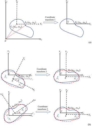
(x_PO, y_PO) is coordinate of point P of the eddy boundary in the earth-centric coordinate system. (x_PC, y_PC) is coordinate of P in the eddy-centric coordinate system. C is eddy center, also the origin of eddy-centric coordinates. Constant λ=111.7(km).

In step 2, the best-fit ellipse was determined by the least-squares method in an ellipse-centric system (the dashed red line in Figure 1(b)); this step was performed for each eddy boundary. We defined the eddy orientation as the acute angle between the X-axes of the two coordinate systems; the value ranged from – 90° to 90°. The eddy boundary was then rotated according to orientation angle θ, so that the major axis of its best-fit ellipse was in the east–west direction of geography. Figure 1(b) shows two cases in which eddies have a negative orientation (the top row) and positive orientation (the bottom row). The equations for coordinate transform 2 are as follows: (4) $x_{PE}=x_{\mathrm{P}\mathrm{C}}\times \mathrm{c}\mathrm{o}\mathrm{s}(\theta )+y_{\mathrm{P}\mathrm{C}}\times \mathrm{s}\mathrm{i}\mathrm{n}\left(\theta \right)$(4) (5) $y_{PE}=-x_{\mathrm{P}\mathrm{C}}\times \mathrm{s}\mathrm{i}\mathrm{n}(\theta )+y_{\mathrm{P}\mathrm{C}}\times \mathrm{c}\mathrm{o}\mathrm{s}\left(\theta \right)$(5)

(x_PE, y_PE) is coordinate of point P in the eddy-centric coordinate system after the rotation of eddy shape. Note that the angle θ in the equations can be positive or negative. In the third step, the mean shape of all horizontally aligned eddies was derived in the eddy-centric coordinate system.

3. Results and discussion

Since the particularity of geographical location and complexity of wind and current system in the SCS, it is necessary to give a description of geographical condition and eddy distribution in the SCS. Figure 2(a) shows the map of the water depth in the SCS. The white line depicts the contour with a depth of 1000 m. Spatial distribution of eddies occurrence at each 0.5°×0.5° latitude-longitude gird is depicted in Figure 2(b). In the SCS, most eddies are observed in areas with water depth deeper than 1000 m. They are most active in the southwest of Taiwan and Luzon island, also the eastern SCS. The pattern distribution is in agreement with the result of He et al. (2018), but the magnitude of eddy number is much higher. This may be caused by the different eddy identification algorithms and thresholds for eddy lifetimes when analyzing eddy data (10 and 28 days respectively). Statistically, the number of eddies with lifetime longer than 10 days is 13599 and 3803 for 28 days. Figure 2(c,d) show the wind fields during the southwest monsoon (May to September) and the northeast monsoon (October to March). The surface currents in the SCS are driven by the monsoon, flowing from southwest to northeast during summer (Figure 2(e)) and in reverse during winter (Figure 2(f)). After understanding the background of the SCS, snapshots of eddy boundaries and their best-fit ellipses are obtained (not shown). The results are the same with Chen, Han, and Yang (2019), indicating that eddy shapes in the SCS with different scales and orientations are closer with ellipses than circles. Using the method in 2.4, statistics of eddy shapes and orientations of mesoscale eddies in the SCS are shown in Figure 3(a)–(f). Figure 3(a) shows the average shape of eddies in the SCS, also overlaid its best-fit ellipse and the average shape of eddies in the global oceans. It should be noted that the effect of the poleward decrease in the zonal distance per longitude is rectified in the Cartesian coordinate (Chen, Han, and Yang 2019). The average shape of eddies in the SCS is approximately equivalent to an ellipse with a semimajor axis (a) of 101.3 km, a semiminor axis (b) of 61.3 km, a focal distance c of 80.6 km, and an eccentricity (e = c/a) of 0.80. The average shape in the SCS is with larger size and eccentricity compared with the mean shape for global ocean eddies reported by Chen, Han, and Yang (2019) (a=87.0 km, b = 54.0 km, e = 0.78). We also obtained the average shape of different classifications of eddies. There are subtle differences between anticyclonic eddies (AEs) and cyclonic eddies (CEs) in Figure 3(c). Mean shape of AEs with a=101.1 km, b=61.9 km, is a little bigger than those of CEs (a=99.7 km, b=62.0 km). When we analyzing eddies live longer than 70 days, the differences of mean shape between AEs and CEs increase. The a and b for AEs are 122.4 and 78.3 km, for CEs are 117.8 and 74.7 km. Westward propagating eddies are around 8 km larger than eastward propagating eddies in semimajor and semiminor axis (Figure 3(e)). Table 1 lists three eddy attributes that are correlated with eddy sizes. Subtle differences are found in the attributes of AEs and CEs. While westward-propagating eddies prefer to live longer lifetimes and own stronger energies than eastward-propagating eddies. They also have longer travel distances and larger sizes. It can infer that stronger energies (with larger EKE) support eddies’ larger sizes and longer distances. Significant relationships between eddy sizes and their lifetimes are found. Table 2 gives a description in detail. Eddy size becomes larger with the increase of eddy lifetime. Zonal average shape in the SCS shows subtle distinctions in eddy size. Eddies in the longitudinal zone 110°E to 113°E have a mean shape with a=114.3 km and b=69.2 km, more than 10 km larger than the average shape in the SCS. This is in agreement with bigger mean radius in this area (He et al. 2018). Correspondingly, mean shape in 119°E to 122°E is around10 km smaller than that of the whole SCS.

Figure 2. Geographical features of the South China Sea. (a) Map of water depths. Bathymetric contour of 1000 m is in white line. (b) Distribution of eddy occurrences. (c,d) are wind fields during Southwest monsoon (May to September) and Northeast monsoon (October to March). (e,f) are current fields during Southwest monsoon and Northeast monsoon.

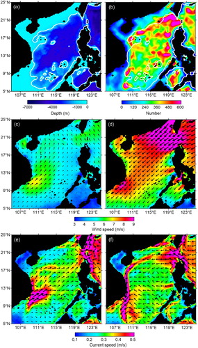
Figure 3. Eddy shapes and eddy orientation maps in the SCS. (a) Average shape of oceanic eddies (blue line) in the SCS, the best-fit ellipse (green line), and the average shape in the global ocean (black line). (b) Radar map of eddy orientation in the SCS based on the number of occurrences. The orientation is based on the major axis of the best-fit ellipses at a given angle with a 5° interval. The red line indicates the dominant eddy orientation. (c,e) show the average shapes of the AEs and CEs and westward – and eastward-propagating eddies, respectively. (d,f) are the radar maps of the eddy orientations of the AEs and CEs and the westward – and eastward-propagating eddies, respectively.

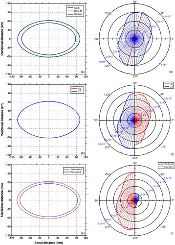
Table 1. Attributes of different classifications of mesoscale eddies.

Attribute	AE	CE	Westward	Eastward
Lifetime (day)	25.91	25.85	27.14	20.70
Distance of trajectory (km)	105.48	105.20	114.92	66.05
EKE (cm^2/s^2)	479.96	518.36	514.46	430.68

Table 2. Size of eddy shape variation with lifetime.

Lifetime	10–30 days	1–3 month	3–6 month	6–9 month	>9 month
a (km)	88.7	104.5	122.3	132.3	129.6
b (km)	54.1	64.7	77.2	87.9	89.8

Statistics about eddy orientations in the SCS are shown in Figure 3(b,d,f). Figure 3(b) represents that mesoscale eddies in the SCS were mainly oriented northeast-southwest, with an angle of 74°/254° (direction of the red line), indicating that the eddy orientation is asymmetric. Chen, Han, and Yang (2019) proposed that the primary orientation for global eddies is 104°/284° (nearly north–south). The eddy orientation maps of the AE verse CE and the westward – verse eastward propagating eddies show the same northeast-southwest orientation. The differences of principle orientations between global and SCS eddies are probably attributed to the complex wind and current conditions. They blow (flow) from southwest to northeast in summer and reverse in winter (Figure 1(c)–(f)). Additionally, the direction of the continents also reflects the eddy orientations. Eddies tend to be parallel with the coastlines along major continents (Chen, Han, and Yang 2019). Chen, Hou, and Chu (2011) proposed that eddies in the northern SCS primarily propagate southwestward along the continental slope.

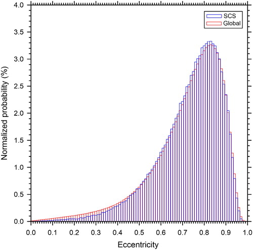
The overall departure of the eddy shape in the SCS from a circle is illustrated in the histogram of the eccentricity of the best-fit ellipses (Figure 4). The corresponding data for global ocean eddies (Chen, Han, and Yang 2019) are also shown in Figure 4. A very small proportion of eddies have a circular shape (eccentricity ≈ 0) in the SCS and the global ocean. The peak values of both histograms are around 0.83. Approximately 60% of the values are in the range of 0.7∼0.9, indicating that the majority of eddies in the SCS have an elliptical structure. The same result is observed for eddies in the global ocean. Compared with the global distribution, eddies in the SCS with eccentricities of 0.51∼0.88 account for a larger proportion, indicating that eddies in the SCS are flatter than those in the global ocean. This is also confirmed by the average eccentricity in the SCS (0.80), larger than the global ocean one (0.78). For the sea area with the same latitude range as the SCS, eccentricity of mean shape in the east Pacific, Bay of Bengal and Arabian Sea are both around 0.78. It demonstrates that the semi-closed geographical conditions of the SCS affect the geometry of mesoscale eddies, making them a slight flatter than eddies in other open oceans.

Figure 4. Normalized histogram of the eccentricity of the best-fit ellipses in an eddy-centric coordinate system for oceanic eddies in the SCS (blue histogram). The black histogram shows the data for the global eddies.

The spatial distribution of the eddy eccentricity based on the average shape of the best-fit ellipse at 0.5°×0.5° resolution is shown in Figure 5(a,b) for westward – and eastward-propagating eddies respectively. Chen, Han, and Yang (2019) proposed the contrast in eccentricity is much larger between eastward – and westward-propagating eddies. The conclusion is also the same in the SCS. Eastward-propagating eddies tend to have lager eccentricity than westward – eddies. Eddy eccentricities are found to be in opposite relationships with their propagation speeds in some certain areas in the SCS. For westward-propagating eddies, they show low-eccentricity band along with the coastline of China, while they travel with higher speeds (see Figure 5(a,c)). The same situations are also found around the Kalimantan Island for both westward-propagating and eastward – eddies. For other areas, the situations are more complex. The attributes of mesoscale eddies are also related to eccentricities. Table 3 shows that eddy eccentricities become lower with the increase of their amplitude and lifetimes. With EKE increasing to around 900 m²s², eccentricities decline, and then fluctuate around an average of 0.77. While the variety of eccentricities under the influence of vorticity are not unidirectional. In vorticity 1.5–2.5, 2.5–10 (10⁻⁶ s⁻¹), eccentricities decline at the first phase, and then increase. After vorticity value of 10 (10⁻⁶ s⁻¹), eddy eccentricities decline again. It’s a reasonable explanation that stronger eddies with more energy tend to live longer.

Figure 5. The geographical distribution eddy eccentricates and propagation speeds. Eccentricates are derived from best-fit eddy ellipses in 0.5°×0.5° grid resolution. All ellipses are averaged in an eddy-centric coordinate system with a horizontal orientation. (a,c) are for westward-propagating eddies. (b,d) are for eastward-propagating eddies.

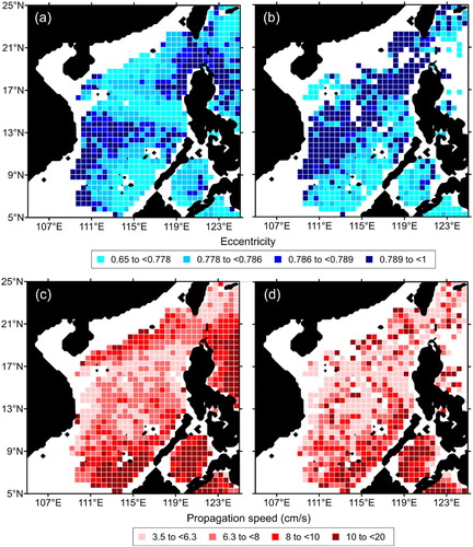
Table 3. Eddy eccentricity variation with attributes.

Amplitude (cm)	6	12	18	24	30
e	0.782	0.775	0.764	0.754	0.745
EKE (m^2s^2)	300	600	900	1200	1500
e	0.782	0.779	0.772	0.774	0.774
Vorticity (10^−6 s^−1)	1.5	2.5	6.5	10.0	12.0
e	0.773	0.760	0.785	0.799	0.796
Lifetime (day)	10–30	30–90	90–180	180–270	>270
e	0.804	0.786	0.776	0.742	0.724

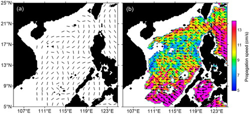
Map of eddy primary orientations with a 1°×1° grid resolution is shown in the Figure 6(a). Along the coast, eddies tend to have orientations in accordance with the land trend. And in the latitudinal zone 19°N to 21°N, they are in horizontal arrangement approximately. Most of them prefer to be in northeast-southwest orientation in the SCS, although a number of them in the direction of northwest-southeast. The results are in agreement with Figure 3(b). From the perspective of latitudinal zone, eddy orientations vary with a small angle regularly. This phenomenon is more obvious in the central SCS, which can be interpreted as rotation of eddy shape proposed by Chen, Han, and Yang (2019). There may be three potential reasons influencing eddy orientations. First, the SCS is a semi-closed ocean. The direction of the coastline plays an important role in eddy propagation and orientations. Eddies in coastal area are in similar directions with the land. Second, eddy orientations are in good agreement with the direction of eddy propagation. Eddies propagate southwestward along the continental slope of the northern SCS (Wang et al. 2008b). He et al. (2018) showed eddies west of Luzon strait propagate westward or northwestward. This result is confirmed in Figure 6(b). Comparisons between Figure 6(a,b) can illustrate that eddy orientations and propagation are consistent with each other. Third, eddy orientations are also driven by the wind and current during their propagations and rotations. Further studies are supposed to focus on the complex and comprehensive functions by eddy propagation and rotation and wind, current direction.

Figure 6. (a) Geographical distribution of the eddy orientation in a 1°×1° grid resolution. (b) Directions and speeds of eddy propagations.

To prepare for our next studies aiming to reveal the dynamic reasons for the eddy geometry, several statistics of eddy geometry under the influence of wind-eddy, current-eddy and eddy-eddy interactions have been carried out. With the increase of velocity, the areas of eddies increase obviously. Correlations between eddy orientations and wind (current) directions are more complex. Data with differences between the wind direction and eddy orientation within 90-degree account for 0.54 and 0.68 for summer and winter, respectively. For current, proportions for summer and winter are 0.72 and 0.52, respectively. Mean shape of interactive eddy pairs is with a=117.8 km, b=71.14 km and e=0.80, which is larger and flatter than non-interactive eddies (a=90.4 km, b=56.8 km and e=0.78). Also, the primary orientation of non-interactive eddies is prominent, with a direction of 72°/252° accounting for 0.8%. In contrast, orientations are in the more uniform distribution for interactive eddies.

4. Implications

Since characteristic eddy shape and orientation are of vital importance for eddy research, it is necessary to examine the role of eddy’s elliptical shape on the spatial patterns of physical and biological parameters and air–sea interactions. Chelton et al. (2011a) proved that eddies cause the co-propagation of CHL distribution and SSH. They obtained distinctly dipole structures composite averages of log₁₀(CHL) fields in the region 18°S to 22°S, 130°W to 80°W. Using the method for the CHL analysis proposed by Chelton et al. (2011a), we obtained the normalized composite CHL structure in the SCS (Figure 7(a,c)). The rotation of the frame of reference is determined by the orientation of the large CHL gradient (see details in Chelton et al. 2011a). As a reference, we also show the composite structure whose rotation was determined by the eddy orientation (Figure 7(b,d)). The circular gradient-rotated composites exhibit a complex pattern with dipoles. Interestingly, the ellipse-based composites exhibit a concentric monopole pattern, indicating that the composite analysis is very sensitive to the eddy geometry. Chelton et al. (2011a) also pointed out that monopole structures with strong physical-biological interactions are within eddy cores sometimes. We believe that the evolution from a circle to an ellipse is an important step in the transformation of the eddy structure. In addition to CHL, we also analyzed the SSTA (Figure 8(a,d)). The dipole structure is apparent in the circular non-rotated composites in the area encompassing twice the radius, whereas the dipole structure is relatively weak in the ellipse-based composites.

Figure 7. Spatial patterns of the eddy-induced chlorophyll variability (Anomaly log₁₀ (CHL)) in the South China Sea and Kuroshio extension (January 1998 – December 2008). The maps on the left are normalized by the CHL gradient. The maps on the right are normalized by the eddy orientation. (a) to (d) are for the SCS and (e)–(f) are for the Kuroshio extension. (a, b, e, f) are the AEs and (c, d, g), and (h) are the CEs.

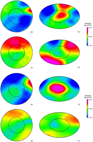
Figure 8. Spatial patterns of the eddy-induced SSTA variability (°C) in the SCS and Kuroshio extension (January 1998 – December 2008). The maps on the left are based on circular non-rotated coordinate system. The maps on the right are based on elliptical rotated coordinate system. (a)–(d) are for the SCS and (e)–(f) are for the Kuroshio extension. (a, b, e, f) are the AEs and (c, d, g, h) are the CEs.

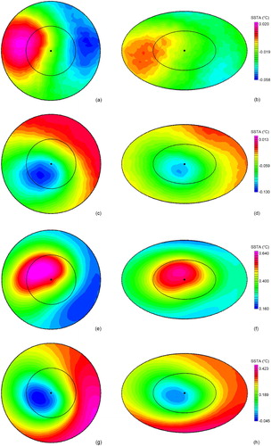
The SCS is a semi-enclosed marginal sea with complex environment as a result of its unique geographical position. For a comparison, the same analysis that was conducted for the CHL (Figure 7(e)–(h)) and SSTA (see Figure 8(e)–(h)) in the SCS was also performed for the Kuroshio extension in the open sea (130°E to 179°E, 25°N to 45°N). For CHL, the gradient-rotated composites show complex CHL structures in the one-radius (1R) circle (Figure 7(e,g)). The monopole with a closed structure is observed in the 1R circle for the eddy-based orientation (Figure 7(f,h)), especially in the AEs. For the SSTA composites, the non-rotated structures exhibit dipole structures in the two-radius (2R) circle. Although the SSTA cores are offset from the eddy center, they are within 1R of the circle and exhibit a closed structure (Figure 8(e,g)). For the ellipse-based composites, the SSTA cores are closer to the eddy core in the meridional direction, and the dipole structure is weaker (see Figure 8(f,h)).

The results of the analysis of the relationship between eddies, CHL, and SSTA in the SCS and Kuroshio extension indicate that eddy shape is sensitive to composite analysis and it is more appropriate to use an elliptical than a circular shape for eddies for the composite analysis. The validity of the elliptical eddy shape is verified. The monopole structure appears to be more common in the open-ocean (Kuroshio extension) than in a semi-enclosed sea (SCS). However, it should be considered that the number of eddy samples in the Kuroshio extension was about 400 thousand, which was about 5 times the number of samples obtained in the SCS. On the other hand, the SCS is a semi-enclosed marginal sea with numerous islands, and due to the lack of open ocean areas in the SCS, the accuracy of eddy identification has been limited.

The spatial patterns of the coupling between SST and sea surface wind speed over mesoscale eddies in the SCS depend largely on the seasonal variations of the SST gradient, the wind speed, and the consistency in the wind direction (Sun et al. 2016). Several studies have investigated the seasonal patterns and the effects of eddies on SSTA and on surface CHL (Chow and Liu 2012; He et al. 2016; Sun et al. 2016). In future studies, we will focus on seasonal eddy characteristics and their effects on SST and surface CHL using the ellipse-based and eddy-centric coordinate system proposed in this study. We will also consider the wind and current directions as correction parameters in the composite analysis.

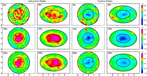
To further verify our elliptical eddy shape result, composite analyses of Argo-measured subsurface sea temperature have been performed. Figure 9 shows temperature anomaly in 20, 100, 300 m for AEs and CEs. Under non-rotated coordinate system, signals of temperature within 1R show several extremums. This is obvious in Figure 9(e,g) etc. Multi-extremums have been revised into a single extreme in the elliptical coordinate system (Figure 9(f,h)). Besides, in the north–south direction, the coupling between the core of temperature and the eddy center is in better agreement (see the comparisons between Figure 9(e,f)). Also, it is worthy to consider the deviation between the temperature and eddy cores. Asymmetry in the east–west direction of mesoscale eddy geometry may bring a new sight of this issue.

Figure 9. Spatial patterns of the eddy-induced subsurface variability (°C) in the SCS (1996-2016). The first and third columns are based on circular non-rotated coordinate system. The second and fourth columns are based on elliptical rotated coordinate system.

5. Conclusion

Based on a long-time series altimeter dataset of SCS eddies (1993-2018), geometric features of mesoscale eddies are obtained. Distributions of eddy eccentricities, orientations show regional characteristics, different from those derived from global eddies. Eddies’ mean shape in the SCS is larger and flatter than that of global eddies. This may be caused by the semi-closed geographical location of the SCS. It is believed that the wind and current can influence eddy geometry in the SCS. While the dynamic reasons for them are still at their beginning stage. The effects on eddy geometry influenced seasonal and intraseasonal variations of winds and currents in the SCS deserve further studies (Wang et al. 2020). Composite analyses on eddy-induced sea temperature and chlorophyll demonstrate the physical and biological effects of eddy geometry. The analyses indicate that geometry of eddies has to be considered because of their important role in the kinematics and dynamics of mesoscale eddies.

Altimeter-derived high-resolution SLA data are well suited for the investigation of oceanic eddies. Our understanding of the eddy geometry has improved thanks to the widely available high-resolution satellite data. The findings obtained in this study are of fundamental importance to eddy characterization in the SCS. Improved understandings of the geometric features of mesoscale eddies in the SCS facilitate future research in the SCS and investigations of the interaction between mesoscale eddies and the atmosphere. They provide important reference data for deep-sea research and pave the way for future research on physical-biological interactions in air–sea coupled systems.

Disclosure statement

No potential conflict of interest was reported by the author(s).

Additional information

Funding

This research was jointly Supported by the National Natural Science Foundation of China [No. 42030406], Marine Science & Technology Fund of Shandong Province for Pilot National Laboratory for Marine Science and Technology (Qingdao) [No. 2018SDKJ0102], and ESA-NRSCC Scientific Cooperation Project on Earth Observation Science and Applications: Dragon 5 [No. 58393].

References

- Amores, A., S. Monserrat, O. Melnichenko, and N. Maximenko. 2017. “On the Shape of sea Level Anomaly Signal on Periphery of Mesoscale Ocean Eddies.” Geophysical Research Letters 44 (13): 6926–6932.
- AVISO. 2016. “SSALTO/DUACS User Handbook: (M) SLA and (M) ADT Near-Real Time and Delayed Time Products.” In: Issue 5.0, AVISO Publ. CLS-DOS-NT-06-034, SALP-MU-PEA-21065-CLS, (29 pp.).
- Bryden, H. L., and E. C. Brady. 1989. “Eddy Momentum and Heat Fluxes and Their Effects on the Circulation of the Equatorial Pacific Ocean.” Journal of Marine Research 47: 55–79.
- Chelton, D. B., P. Gaube, M. G. Schlax, J. J. Early, and R. M. Samelson. 2011a. “The Influence of Nonlinear Mesoscale Eddies on Near-Surface Oceanic Chlorophyll.” Science 334: 328–332.
- Chelton, D. B., M. G. Schlax, and R. M. Samelson. 2011b. “Global Observations of Nonlinear Mesoscale Eddies.” Progress in Oceanography 91: 167–216.
- Chen, G., G. Han, and X. Yang. 2019. “On the Intrinsic Shape of Oceanic Eddies Derived from Satellite Altimetry.” Remote Sensing of Environment 227: 75–89.
- Chen, G., Y. Hou, and X. Chu. 2011. “Mesoscale Eddies in the South China Sea: Mean Properties, Spatiotemporal Variability, and Impact on Thermohaline Structure.” Journal of Geophysical Research-Oceans 116: C06018.
- Chow, C. H., and Q. Liu. 2012. “Eddy Effects on Sea Surface Temperature and Sea Surface Wind in the Continental Slope Region of the Northern South China Sea.” Geophysical Research Letters 39 (2): 2601.
- Early, J. J., R. Samelson, and D. B. Chelton. 2011. “The Evolution and Propagation of Quasigeostrophic Ocean Eddies.” Journal of Physical Oceanography 41: 1535–1555.
- Faghmous, J. H., I. Frenger, Y. Yao, R. Warmka, A. Lindell, and V. Kumar. 2015. “A Daily Global Mesoscale Ocean Eddy Dataset from Satellite Altimetry.” Scientific Data 2: 150028. doi:10.1038/sdata.2015.28.
- Frenger, I., N. Gruber, R. Knutti, and M. Munnich. 2013. “Imprint of Southern Ocean Eddies on Winds, Clouds and Rainfall.” Nature Geoscience 6 (8): 608–612.
- He, Q., H. Zhan, S. Cai, and Z. Li. 2016. Eddy Effects on Surface Chlorophyll in the Northern South China Sea: Mechanism Investigation and Temporal Variability Analysis. Deep-Sea Research Part I-Oceanographic Research Papers, S0967063715301230.
- He, Q., H. Zhang, S. Cai, Y. He, G. Huang, and W. Zhan. 2018. “A New Assessment of Mesoscale Eddies in the South China Sea: Surface Features, Three-Dimensional Structures, and Thermohaline Transports.” Journal of Geographical Research-Oceans 123 (7): 4906–4929.
- Hu, J., H. Kawamura, H. Hongi, and Y. Qi. 2000. “A Review on the Currents in the South China Sea: Seasonal Circulation, South China Sea Warm Current and Kuroshio Intrusion.” Journal of Oceanography 56: 607–624.
- Jia, Y., and E. P. Chassignet. 2011. “Seasonal Variation of Eddy Shedding from the Kuroshio Intrusion in the Luzon Strait.” Journal of Oceanography 67 (5): 601–611.
- Le Vu, B., A. Stegner, and T. Arsouze. 2018. “Angular Momentum Eddy Detection and Tracking Algorithm (AMEDA) and its Application to Coastal Eddy Formation.” Journal of Atmospheric and Oceanic Technology 35: 739–762.
- Li, Q., L. Sun, S. Liu, T. Xian, and Y. Yan. 2014. “A new Mononuclear Eddy Identification Method with Simple Splitting Strategies.” Remote Sensing Letters 5: 65–72.
- Lin, X., C. Dong, D. Chen, et al. 2015. “Three-dimensional Properties of Mesoscale Eddies in the South China Sea Based on Eddy-Resolving Model Output.” Deep-Sea Research Part I-Oceanographic Research Papers 99: 46–64.
- Lin, P., W. Fang, Y. Chen, and X. Tang. 2007. “Temporal and Spatial Variation Characteristics on Eddies in the South China Sea, PartI. Statistical Analyses (in Chinese with English Abstract).” Acta Oceanologica Sinica 29: 14–22.
- Liu, Y., G. Chen, M. Sun, S. Liu, and F. Tian. 2016. “A Parallel SLA-Based Algorithm for Global Mesoscale Eddy Identification.” Journal of Atmospheric & Oceanic Technology 33 (12): 2743–2754.
- Liu, Q., A. Kaneko, and J. Su. 2008. “Recent Progress in Studies of the South China Sea Circulation.” Journal of Oceanography 64 (5): 753–762.
- Mason, E., A. Pascual, and J. C. McWilliams. 2014. “A New Sea Surface Height-Based Code for Oceanic Mesoscale Eddy Tracking.” Journal of Atmospheric & Oceanic Technology 31: 1181–1188.
- McGillicuddy, D. J., L. A. Anderson, N. R. Bates, T. Bibby, K. O. Buesseler, C. A. Carlson, C. S. Davis, et al. 2007. “Eddy/Wind Interactions Stimulate Extraordinary mid-Ocean Plankton Blooms.” Science 316: 1021–1026.
- Nencioli, F., C. Dong, T. Dickey, L. Washburn, and J. C. McWilliams. 2010. “A Vector Geometry-Based Eddy Detection Algorithm and its Application to a High-Resolution Numerical Model Product and High-Frequency Radar Surface Velocities in the Southern California Bight.” Journal of Atmospheric & Oceanic Technology 27: 564–579.
- Qu, T. D. 2000. “Upper-layer Circulation in the South China Sea.” Journal of Physical Oceanography 30: 1450–1460.
- Su, J. 2004. “Overview of the South China Sea Circulation and its Influence on the Coastal Physical Oceanography Near the Pearl River Estuary.” Continental Shelf Research 24: 1745–1760.
- Sun, S., Y. Fang, B. Liu, and G. Tana. 2016. “Coupling Between SST and Wind Speed Over Mesoscale Eddies in the South China Sea.” Ocean Dynamics 66 (11): 1467–1474.
- Sun, M., F. Tian, Y. Liu, and G. Chen. 2017. “An Improved Automatic Algorithm for Global Eddy Tracking Using Satellite Altimeter Data.” Remote Sensing 9 (3): 206.
- Wang, G., D. Chen, and J. Su. 2008a. “Winter Eddy Genesis in the Eastern South China Sea due to Orographic Wind-Jets.” Journal of Physical Oceanography 38: 726–732.
- Wang, G., J. Li, C. Wang, and Y. Yan. 2012. “Interactions among the Winter Monsoon, Ocean Eddy and Ocean Thermal Front in the South China Sea.” Journal of Geophysical Research-Oceans 117: C8.
- Wang, G., J. Su, and P. C. Chu. 2003. “Mesoscale Eddies in the South China Sea Observed with Altimeter Data.” Geophysical Research Letters 30 (21): 2121.
- Wang, D., H. Xu, J. Lin, and J. Hu. 2008b. “Anticyclonic Eddies in the Northeastern South China Sea During Winter 2003/2004.” Journal of Oceanography 64 (6): 924–935.
- Wang, Q., L. Zeng, Y. He, and W. Zhou. 2020. “The Linkage of Kuroshio Intrusion and Mesoscale Eddy Variability in the Northern South China Sea: Subsurface Speed Maximum.” Geophysical Research Letters 47 (11): e2020G. L087034.
- Xiu, P., F. Chai, L. Shi, H. Xue, and Y. Chao. 2010. “A Census of Eddy Activities in the South China Sea During 1993-2007.” Journal of Geophysical Research-Oceans 115: C03012.
- Yi, J., Z. Liu, Y. Du, D. Wu, C. Zhou, H. Wei, K. Xu, and F. Liang. 2014. “A Gaussian-Surface-Based Approach to Identifying Oceanic Multi-Eddy Structures from Satellite Altimeter Datasets.” In: Proceedings of the 22nd International Conference on Geoinformatics, Kaohsiung, 2014, pp. 1–5. doi:10.1109/GEOINFORMATICS.2014.6950840.
- Zhang, Z., W. Wang, and B. Qiu. 2014. “Oceanic Mass Transport by Mesoscale Eddies.” Science 345 (6194): 322–324. doi:10.1126/science.1252418.
- Zu, T., D. Wang, C. Yan, I. Belkin, W. Zhuang, and J. Chen. 2013. “Evolution of an Anticyclonic Eddy Southwest of Taiwan.” Ocean Dynamics 63 (5): 519–531.