An investigation on microwave transmissivity at frequencies of 18.7 and 36.5 GHz for diverse forest types during snow season

ABSTRACT

Forests have invariably been considered as an obstacle in retrieving land surface parameters from spaceborne passive microwave brightness temperature (T_B) observations. For quantifying the effect of forests on microwave signals, several models have been developed. However, these models rarely reveal the dependence of microwave radiation on forest types, which can hardly meet the needs of high-accuracy retrieval of terrestrial parameters in forested regions. A ground-based microwave radiometric observation experiment was designed to investigate the dependence of microwave radiation on frequency, polarization, and forest type. Downward T_B at 18.7- and 36.5-GHz for horizontal- and vertical-polarization from the forest canopy was measured at 14 sample plots in Northeast China, along with snowpack and forest structural parameters. By providing fits to experimental data, new empirical transmissivity models for three forest types were developed, as a function of woody stem volume and depending on the frequency/polarization. The proposed models give diverse asymptotic transmissivity saturation levels and the corresponding saturation point of woody stem volume for different forest types. Root-mean-square error results between T_B simulations and Advanced Microwave Scanning Radiometer-2 observations are approximately 3–6 K. This study provides an experimental and theoretical reference for further development of inversion models for snow parameters in forested areas.

KEYWORDS:

• Forest transmissivity
• snow
• woody stem volume
• microwave radiometry
• HUT

1. Introduction

Snow plays an essential role in various human activities and is vital for maintaining the balance of the global water cycle. More than one-sixth of the world’s population living in snow-dominated areas rely on glaciers and seasonal snow packs for their water supply (Barnett, Adam, and Lettenmaier 2005). It also exerts a significant impact on the Earth's surface energy balance and surface-atmosphere interaction through its high albedo and low thermal conductivity (Groisman, Karl, and Knight 1994). Therefore, the ability to accurately retrieve the properties of snow is a meaningful scientific endeavor. Over the course of last 40 years, spaceborne passive microwave (PMW) remote sensing has been widely applied to estimate snow parameters (Ulaby, Moore, and Fung 1986; Mätzler 1987; Roy et al. 2004), such as snow depth (SD) and snow water equivalent (SWE). Crucial progress has been made in the retrieval of SWE over flat and non-vegetated areas (Tait 1998; Derksen, Walker, and Goodison 2005; Goodison and Walker 2020).

However, the presence of forests creates considerable uncertainties and errors in the estimates of snow parameters because of their strong microwave attenuation and emission capabilities (Hall, Foster, and Chang 1982; Chang, Foster, and Hall 1996; Pampaloni 2004; Langlois, Royer, and Goïta 2010; Tedesco and Narvekar 2010). The effect of forests on the retrieval accuracy of snow parameters in earlier studies was typically mitigated by introducing the forest cover fraction as a correction factor in algorithms (Foster et al. 1991; Chang, Foster, and Hall 1996). Even though quite a few progresses have been made in recent years in the development and application of empirical or semi-empirical models to reduce forest impacts (Derksen 2008; Roy et al. 2012; Cohen et al. 2015), high-accuracy retrieval of snow parameters in forested areas remains a huge challenge (Larue et al. 2017). Parameterization of simplified models for different area under diverse forest conditions is an effective and practical way at current stage to solve the problems related to the influence of forest on the satellite SD/SWE retrieval. Therefore, modeling the microwave radiation and scattering characteristics of forests has been considered extremely paramount for the accurate retrieval of snow parameters in forests (Mätzler 2006).

Mo et al. (1982) proposed the τ-ω model, which is deemed suitable for modeling the microwave transfer properties of forest canopies with multiple scattering, provided that it uses effective (or equivalent) parameters and is calibrated through a theoretical multiple scattering model (Ferrazzoli, Guerriero, and Wigneron 2002; Kurum et al. 2011). One of the main variables which they used to parameterize the forest, the forest transmissivity (γ), is closely related to the optical thickness (τ) of the forest. γ is defined as the portion of electromagnetic radiation penetrating the forest canopy, that is, the extent to which the canopy attenuates radiation. To make the effects of forest on microwave signals be quantified, researchers have conducted several field campaigns, including ground-based observations (e.g. Mätzler 1994; Pardé, Royer, and Vachon 2005; Li et al. 2019), airborne measurements (Kruopis et al. 1999; Foster et al. 2005; Derksen et al. 2009), and satellite data usage (Derksen, Walker, and Goodison 2003, 2005). Among them, a considerable part of the research aims to establish a relationship model between γ and woody stem volume (Vol) or vegetation index to modify the forest effect. For example, Langlois et al. (2011) defined γ as a function of Vol and depended on the frequency/polarization based on an experiment with an airborne microwave radiometer conducted in a large area. Vander Jagt et al. (2015) estimated γ by using airborne T_B variability and a globally available vegetation dataset. Recently, based on long-term series radiometer measurements targeting a single Scots Pine, Li et al. (2019, 2020) proposed an empirical model between tree skin temperature and γ to reveal the sensitivity of γ to physical temperature. However, most of the values of τ (or γ) and the single scattering albedo (ω) were derived from observational data of a specific type of forests, with limited variability in forest structural properties. In addition, few studies have reported on the regional-scale variations in microwave emissions from both coniferous and deciduous forests. As a result, the values for τ and ω retrieved from a single tree or forest type may not be applicable to other forest types.

This study aims to explore variations in γ under various types of forests by experimental observation. To further elucidate the microwave radiative transfer process, new transmissivity models for diverse forest types in Heilongjiang province, Northeast China have been developed as a function of Vol depending on the frequency/polarization. The performance of these new transmissivity models incorporated into the forward model for simulating satellite T_B have been evaluated. Furthermore, the error analysis and sources of uncertainty in the process of forest transmissivity measurements have been discussed. Therefore, this study provides an experimental and theoretical reference for further development of the inversion models for forest snow coupling system.

2. Materials and methods

2.1. The study area

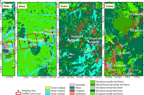
The study area is located in the Daxing’anling Mountain area and Xiaoxing’anling Mountain area in Heilongjiang province, Northeast China (121.819–129.857°E, 47.745–53.175°N). According to the geographic locations and climate types, four representative study sites were selected from the study area: Huma, Mohe, Yichun, and Xunke. Figure 1 displays the locations and climate types of the sampling sites. Huma and Mohe are located in the northern temperate zone of the Genhe region, whereas Yichun and Xunke are located in the temperate zone of the Xiaoxing’an region. The study area includes many typical tree species, such as pine, larch, spruce, fir, birch, and Mongolian oak. Figure 2 demonstrates the land cover type of the AMSR-2 pixels where sampling sites locate. The following conditions need to be met for the selection of tree sample plots: fairly high forest cover fraction (as shown in Figure 2), dense tree distribution, relatively flat terrain, as well as away from electromagnetic interference sources.

Figure 1. Location map of the study area showing the different climate types of the sampling sites. Data source: Resource and Environmental Science and Data Center (http://www.resdc.cn).

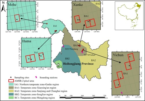
Figure 2. Land cover type of the AMSR-2 pixels where sampling sites locate. Data source: ChinaCover2010, National Earth System Science Data Sharing Infrastructure, National Science & Technology Infrastructure of China (http://www.geodata.cn).

2.2. Data sources

2.2.1. Ground-based radiometric measurements

Experimental observations of the microwave downward brightness temperature (T_B) from the forest canopy of 14 sites were made from December 15, 2016, to December 29, 2016. The downward T_B of the forest canopy was observed with incidence angles of 40°, 50° and 60°, using two ground-based movable upward-pointing microwave radiometers (JYRS-K and JYRS-Ka, JingYuetan Remote Sensing experiment station radiometer-K (Ka) band). The JYRS-K and JYRS-Ka microwave radiometers were designed and manufactured by the microwave remote sensing research group of the Northeast Institute of Geography and Agroecology (IGA) of the Chinese Academy of Sciences (CAS). The measurement center frequencies are 18.7- and 36.5-GHz in horizontal (H) and vertical (V) polarizations, respectively. The intermediate frequency bandwidth for each frequency was 200 MHz and 400 MHz, respectively. For both frequencies, the absolute system stability of JYRS-K and JYRS-Ka was 2.0 K, sensitivity 1.0 K. The antenna-type implemented is a diagonal low sidelobe horn antenna with a half-power beamwidth of 15.0°. Before initiating a new series of observations, the radiometers were calibrated with warm (ambient temperature microwave absorber) and cold (liquid nitrogen) targets, as described by (Song, Zhao, and Guan 2008). At each observation site, the K band (18.7 GHz) and Ka band (36.5 GHz) radiometers were mounted on two 1.2 m high tripods for acquiring simultaneous observations, with the receiving antennas facing upward towards the forest canopy (Figure 3). Owing to the uneven spatial distribution of trees in natural forests, observational measurements at 2–4 azimuth angles at 90° intervals (0°, 90°, 180°, and 270°) were implemented to reduce the observational error. The starting azimuth angle 0° here refers to the first observational direction at each site, which differs from the consensus that the reference vector points to true north. The incidence angle ranged from 40° to 60° with steps of 10°. The T_B observation period was controlled in the time range of 10:00 am to 2:00 pm local time on each day. In most cases, only one site was observed in one day, and at each site, the measurement took about 2 h. The T_B observations were also supported by in situ measurements of Vol, snow properties, along with physical temperature of the environment, trees, and snow. The measurement parameters of the snow profiles and structural characteristics of the forest are summarized in Table 1.

Figure 3. Configuration of the radiometer observations viewed from (a) side and (b) front; and (c) description of the measured T_B from the canopy.

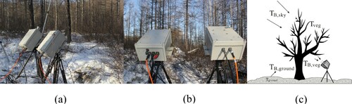
Table 1. Parameters of forest canopies and snow profiles for each tree sample plot.

		Forest characteristic parameters						Snow characteristic parameters
Sample plot	Date of observation	Stand density (trees/ha)	Height (m)	Woody stem volume (m³/ha)	Broad leaf forest (%)	Needle leaf forest (%)	Dominant tree species/forest type	Air temperature (°C)	Snow depth (m)	Snow density (g/cm³)	Effective snow grain diameter (mm)	Snow temperature (°C)
Huma01	2016/12/15	850	12	70	0	100	DNF	–14	0.19	0.131	1.13	–13.5
Huma02	2016/12/16	3316	12.5	153	22	78	DNF	–12	0.19	0.127	1.06	–12.4
Huma03	2016/12/17	1118	10.3	53	4	96	DNF	–5	0.16	0.113	1.06	–9.2
Huma04	2016/12/18	2150	12.6	135	7	93	DNF	–14.5	0.16	0.126	1.16	–12.8
Huma05	2016/12/19	1421	15.5	156	0	100	DNF	–18	0.14	0.145	1.2	–15.8
Mohe01	2016/12/20	3266	10.7	104	75	25	DBF	–19	0.14	0.15	1.23	–12.9
Yichun01	2016/12/23	2500	12	125	36	64	GNF	–18	0.19	0.139	1.3	–11
Yichun02	2016/12/24	2267	15.5	234	0	100	DNF	–16	0.17	0.14	1.28	–12.8
Yichun03	2016/12/25	1704	14	205	12	88	GNF	–13	0.2	0.156	1.39	–10.6
Yichun04	2016/12/26	901	18.4	292	28	72	DNF	–17.5	0.23	0.13	1.38	–12.4
Xunke01	2016/12/27	3209	12.6	153	94	6	DBF	–14.5	0.23	0.157	1.42	–13.3
Xunke02	2016/12/28	1592	10	100	93	7	DBF	–16	0.21	0.141	1.41	–10.8
Xunke03	2016/12/29	2821	9.4	98	93	7	DBF	–15	0.21	0.148	1.45	–11.6
Xunke04	2016/12/29	1078	9.3	28	100	0	DBF	–16	0.25	0.155	1.42	–11.3

2.2.2. Forest measurements

The forest inventories were conducted based on a fixed-area sampling plot approach. For each site, a 20 m × 20 m tree sample plot within the instantaneous field of view of the radiometer antenna was demarcated by the ropes. The total tree height and the diameter at breast height (DBH of 1.30 m) of each tree were also measured. Data from 1147 trees in 14 plots were collected. For each sample plot, all the trees were counted to determine the stand density $\left({\rho }_{plot}\right)$, (1) ${\rho }_{plot}=N_{tree}/S_{plot}$(1) where, $N_{tree}$ represents the number of trees in the plot and $S_{plot}$ represents the area (in hectares) of the plot. The Vol (in cubic meters per hectare) was calculated by the average experimental form factor method proposed by Lin (1964), using the following equations: (2) $Vo{l}_{sl}=f_{∍}\cdot g_{1.3}\cdot \left(H+3\right)$(2) (3) $Vol=\sum _{i=1}^{N}Vo{l}_{sli}/S_{plot}$(3) where, Vol_sl represents the volume of each tree stem (in m³), g_1.3 represents the cross-sectional area at breast height (∼1.3 m) of the trunk, H represents the total tree height (in m), and $f_{∍}$ represents the experimental form factor. The average experimental form factor of the main tree species in China is shown in Table 2 (Lin 1964). In this study, $f_{∍}$ for DBF, DNF and GNF were 0.40, 0.41, and 0.43, respectively. Compared with the methods of species-sensitive volume table, the average experimental form factor method is easy to use, especially in the absence of any tree volume table as reference. In addition, it can not only simplify the measurement process to save labor costs, but also meet the general production requirements for accuracy. The deviation of system disturbance can be within 5% for the majority of tree species (Lin 1964).

Table 2. Average experimental form factor $\left(f_{∍}\right)$ of the main tree species in China

Form factor level	Tree species	Experimental form factor	Applicable tree species
I	Coniferous tree	0.45	Yunnan pine, fir and general strong shade-tolerant coniferous species
II		0.43	Seeding Chinese fir, spruce and general shade-tolerant coniferous species
III		0.42	Chinese fir (regardless of origin), Korean pine, Huashan pine, Huangshan pine and general neutral coniferous species
IV		0.41	Plugged fir, Tianshan spruce, willow fir, Xingan larch, Xinjiang larch, camphor pine, red pine, black pine, oil pine and general light-loving coniferous species
V	Broad-leaved tree	0.40	Poplar, birch, willow, linden, ash, Mongolian oak, oak, cycad, acacia, elm, camphor, eucalyptus and other general broadleaf species, mixed broadleaf forests in Hainan, Yunnan, etc.
VI	Coniferous tree	0.39	Masson pine and general strong light-loving coniferous species

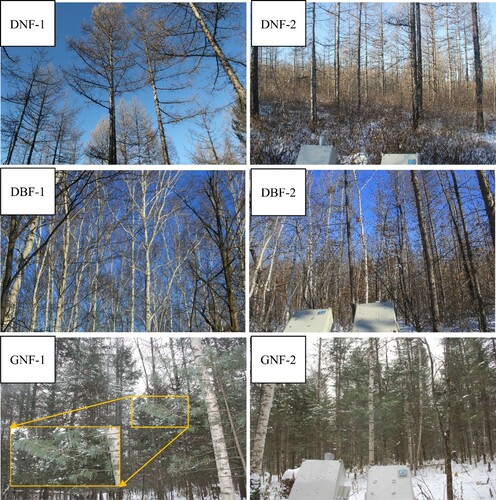
Figure 4 presents the Vol and composition of tree species in each sample plot. The Huma region, with five sampling sites, is dominated by Larch, whereas tree species of the plots in Mohe and Xunke mainly consisted of DBF trees, such as birch, aspen, and Mongolian oak. Compared with the other three regions, the tree species varied greatly in composition in Yichun, including all of DBF, DNF and GNF trees. The tree height, Vol, and stand density in the whole study area ranged from 9 to 18 m, 28–292 m³/ha, and 850–3300 trees/ha, respectively. Figure 5 demonstrates the radiometric measurement scenarios for different forest types, where a local enlargement of the canopy is shown on the left (DNF/DBF/GNF-1), and a general schematic of the antenna observation against the canopy on the right (DNF/DBF/GNF-2). As seen from these photographs, the branches of DBF trees inclined much fewer to the horizontal direction than the DNF and GNF trees. The difference between DNF and GNF is, although they both have branches of similar inclination angle, leaves were remained on GNF in winter which can result in strong attenuation on microwave radiation.

Figure 4. Composition of tree species and woody stem volume at each tree sample plot.

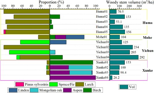
Figure 5. Photos of radiometric measurements corresponding to different forest types.

2.2.3. Snow measurements

Snow pits were dug near at each tree sample plot, and the snow wall was prevented from direct solar illumination from the south. The snow thickness, grain size, and temperature profiles within each natural layer were measured from the surface to snow–soil interface. Each snow layer was visually determined based on variations in the snow grain size profile or thin crust layer (< 0.5cm). Bulk SWE was measured by using a snow coring tube at each site. Macro-photographs of snow grains of each layer were taken against a 1mm reference plate using a digital camera. The greatest extent of the prevailing or characteristic grains (D_m, in mm) was measured from the photographs on computer screen. According to Kontu and Pulliainen (2010), an empirical correction (Eq. (4)) was used in this study to translate D_m to an effective microwave grain size (D_eff, in mm) with the purpose of alleviating large errors arising from the use of Dm in model simulations. (4) $D_{eff}=1.5\cdot \left(1-e^{-1.5\cdot D_m}\right)$(4) Snow was dry all over the profiles, and all the stratification parameters were weighted and averaged to characterize the entire snowpack. The snowpack under forest consisted of 2–4 layers with effective grain sizes and densities ranging from 1.06–1.45 mm and 0.11–0.16 g/cm³, respectively. The SD ranged from 14 to 25 cm, corresponding to SWE values of 26.8$\pm$6.21 mm, the weighted temperature of the snow layer ranged from –9 to –16 °C, and air temperature from –5 to –19 °C. We made an assumption that the snow properties and physical temperature were constant near each site, with air temperature as a proxy for tree temperature.

2.2.4. Sounding data

The downward radiation from the sky $\left(T_{B,sky}\right)$ was calculated using the atmospheric radiation transfer model, i.e. the millimeter-wave propagation model (MPM) proposed by Liebe (1989), and the atmospheric parameters were estimated from sounding data. The university of Wyoming (UWYO) provides an archive of worldwide radio sounding data (freely available at http://weather.uwyo.edu/upperair/sounding.html). The UWYO soundings together with the Integrated Global Radiosonde Archive (https://www.ncdc.noaa.gov/data-access/weather-balloon/integrated-global-radiosonde-archive) have the same raw soundings. The UWYO radiosonde data is directly obtained from the NOAAPORT satellite feed (Larry Oolman, personal communication). The data set includes meteorological elements of standard isobaric surface, temperature and humidity characteristic layer along with wind characteristic layer, which are observed daily at UTC 00:00 and 12:00. For this study, the sounding data was collected in stations 50557 (in Nenjiang city, 49.16 °N, 125.23 °E) and 50774 (in Yichun city, 47.71 °N, 128.90 °E), geographically located as manifested in Figure 1. Station 50557 is about 290 kilometers from the study site Huma, and about 450 kilometers from Mohe. The 50774 station is 30 kilometers away from Yichun and 130 kilometers from Xunke. The meteorological elements used in the MPM model as inputs included atmospheric pressure, geopotential height, temperature, dew point temperature, frost point temperature, and relative humidity.

2.2.5. Satellite observation

The satellite-scale observed T_B throughout the entire observation period is obtained from the Advanced Microwave Scanning Radiometer 2 (AMSR-2) onboard the Global Change Observation Mission 1st-Water (GCOM-W1) satellite (http://gcom-w1.jaxa.jp). L3 ascending daily products have been used in this study, corresponding to each observation date with both frequencies (18.7- and 36.5-GHz) and polarizations (H and V), with a nominal resolution of 0.1° × 0.1° (approximately 10 km × 10 km). The incidence angle θ of the AMSR-2 satellite sensor was 55°. The AMSR-2 pixels, where the sample plots locate, were selected for the implementation of the study.

2.3. Model descriptions

2.3.1. Estimation of transmissivity from the radiometric measurements

Following the law of conservation of energy, the total downward T_B $\left(T_{B,veg,\downarrow }\right)$ towards the radiometer antenna (see Figure 3(c)) is composed of three parts (Ulaby, Moore, and Fung 1986): the downward sky radiation that passes through the forest canopy $({\gamma }^{f,p}\cdot T_{B,sky})$, the thermal emission of the canopy $\left(\right(1-{\gamma }^{f,p}-r_{veg})\cdot T_{veg})$, and the upward ground (snow-soil layer) surface emission reflected back down by the bottom of the canopy $(r_{veg}\cdot T_{B,ground-r})$. $T_{B,veg,\downarrow }$ can be expressed as: (5) $T_{B,veg,\downarrow }=(1-{\gamma }^{f,p}-r_{veg})\cdot T_{veg}+{\gamma }^{f,p}\cdot T_{B,sky}+r_{veg}\cdot T_{B,ground-r}$(5) (6) $r_{veg}={\omega }_{veg}\cdot \left(1-{\gamma }^{f,p}\right)$(6) where γ is the effective forest canopy transmissivity, f represents different frequencies (e.g. f = {18.7, 36.5} GHz), p represents horizontal and vertical polarizations p = {H, V}, $r_{veg}$ is the reflectivity at the bottom of the forest canopy, $T_{veg}$ is the equivalent physical temperature (K) of the forest canopy, and ${\omega }_{veg}$ is the effective scattering albedo of the forest canopy. As the value of $r_{veg}$ is typically small, it is conventionally used as a simplified method, considering the forest canopy as an attenuation layer, ignoring the scattering effect in emission models (Mätzler 1994; Langlois et al. 2011) By following the simplified approach of Mätzler (1994), γ can be estimated from: (7) ${\gamma }^{f,p}\approx \frac{T_{veg}-T_{B,veg,\downarrow }}{T_{veg}-T_{B,sky}}$(7) For a Lambertian surface below a horizontally stratified atmosphere, $T_{B,sky}$ can be modeled at a certain incidence angle, following the work introduced in Section 2.3.2.

The angular correction angular correction proposed by Pulliainen, Grandell, and Hallikainen (1999) is as follows: (8) ${\gamma }^{f,p,{\theta }_2}=({\gamma }^{f,p,{\theta }_1}{)}^{\cos {\theta }_1/\cos {\theta }_2}$(8) Note that, Eq. (8) not only assumed the Lambertian scattering of the forest canopy, but also neglected the possible difference of penetration path of the microwave when the forest was observed at different angles.

2.3.2. Forward model of spaceborne T_B simulation

To demonstrate the performances of new forest transmissivity models under three forest types developed in this study (see Section 3.2), we considered a forward model nested with the new γ–Vol relationships to simulate the spaceborne T_B. From a satellite remote sensing perspective, the top-of-atmosphere T_B of a snow-covered forest scene $\left(T_{B,scene}\right)$ can be described by using the general radiative transfer equation (RTE) (Pellarin et al. 2003) as: (9) $T_{B,sat}=t_{atm}\cdot T_{B,scene}+\left(1-e_{scene}\right)\cdot T_{B,atmdown}+T_{B,atmup}+T_{\cos mic}\cdot t_{atm}^2\cdot \left(1-e_{scene}\right)$(9) All the terms in Eq. (9) are functions of frequency and incidence angle θ between the line of sight and the local normal to the earth surface, $e_{scene}$ is the emissivity of the ground scene, $T_{\cos mic}$ = 2.7 K is the cosmic background radiation, $t_{atm}$ is the atmospheric transmissivity, and $T_{B,atmdown}$ and $T_{B,atmup}$ are the downward and upward atmospheric radiation, respectively, which are considered to be approximately equal in this study.

The atmospheric effects ($T_{B,atmdown}$, $T_{B,atmup}$ and $t_{atm}$) were estimated using the MPM model and the 7-parameter double Debye model (Liebe, Hufford, and Manabe 1991), which is a complex permittivity model of pure water. To obtain $T_{B,atmdown}$, we calculated the emissivity and atmospheric opacity of each atmospheric layer for various observation angles. The downward radiation of each layer is summed according to the relationship between the emissivity and optical thickness. At each frequency, $T_{B,atmdown}$ can be expressed as follows: (10a) $T_{B,atmdown}\left(\theta \right)=(1-\exp (-{\tau }_{d,atm}\left(\theta \right)\left)\right)\cdot T_{mr}+T_{\cos mic}\cdot \exp (-{\tau }_{d,atm}(\theta \left)\right)$(10a) (10b) $T_{mr}=\frac{{\int }_0^{h}T\left(z\right)d\left(\exp \left(-{\tau }_{d,atm}\left(\theta \right)\right)\right)}{{\int }_0^{h}d\left(\exp \left(-{\tau }_{d,atm}\left(\theta \right)\right)\right)}$(10b) where, ${\tau }_{d,atm}\left(\theta \right)$ is the atmospheric optical thickness in the incidence angle θ ${\tau }_{d,atm}\left(\theta \right)={\tau }_{n,atm}/cos\left(\theta \right)$, ${\tau }_{n,atm}$ is the optical thickness at nadir and is the integral expression of the extinction coefficient, including the absorption and scattering coefficients of water vapor and oxygen. $t_{atm}$ is defined as $t_{atm}=\exp \left(-{\tau }_{d,atm}\left(\theta \right)\right)$. $T_{mr}$ is the average T_B of the atmosphere (in Kelvin), z is the path length in km, T (z) is the temperature (K) at the point z, and $T_{B,sky}$ is calculated as the sum of the downward atmospheric radiation $\left(T_{B,atmdown}\right)$ and extra-terrestrial radiation $(T_{\cos mic}=2.7K)$ attenuated in the atmosphere. The input parameters of the model were derived from sounding data. The simulated results manifested that $T_{B,sky}$ ranged from 8 to 10 K at 18.7 GHz and 16–19 K at 36.5 GHz for an incidence angle of 50°.

The $T_{B,scene}$, which includes the contributions of snow, soil, and forests, can be simulated by the commonly-used HUT snow emission model (Pulliainen, Grandell, and Hallikainen 1999) embedded in with the rough bare soil reflectivity model (Wegmuller and Mätzler 1999) and forest transmissivity model. For modeling the effect of snow microstructure on the scattering of microwave radiation in the HUT snow emission model, two empirical equations are applied to relate snow extinction coefficient (${\kappa }_e$, in dB/m) to frequency (f, in GHz) and snow grain size (D_eff, in mm). (11a) ${\kappa }_{e\mathrm{\_}Hallikainen}=0.0018\cdot f^{2.8}\cdot D_{eff}^2$(11a) (11b) ${\kappa }_{e\mathrm{\_}Roy}=2\cdot (f^4\cdot D_{eff}^6{)}^{0.2}$(11b) The parameters of Eq. (11a) were chosen based on laboratory measurements of snow slabs at 18–60 GHz frequency range in Southern Finland (Hallikainen, Ulaby, and Van Deventer 1987). The other semi-empirical Eq. (11b) was suggested by Roy et al. (2004) based on their field measurements in Canada.

For the $T_{B,scene}$ at the top of the canopy within a PMW pixel (AMSR-2 grid cell), the impact of the forest fraction needs to be considered; therefore, the $T_{B,scene}$of a mixed pixel (forested and non-forested areas) can be expressed as follows: (12) $T_{B,scene}=\left(1-ff\right)\cdot T_{B,snow}+ff\cdot T_{B,forest}$(12) In this equation, $ff$ is the forest fraction, $T_{B,snow}$ and $T_{B,forest}$ are the T_B of non-forested and forested areas covered with snow, respectively. Fractions of forested areas of PMW pixels were obtained from land cover data (ChinaCover 2010, http://www.geodata.cn) provided by National Earth System Science Data Sharing Infrastructure, National Science & Technology Infrastructure of China (Zhang et al. 2014).

3. Results and analysis

3.1. Comparison of transmissivity for different forest types measured by radiometer

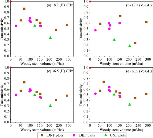
Since we did not directly measure the transmissivities at 55° incidence angle, the spline interpolation method is used to obtain target values. Figure 6 presents the values of transmissivity provided by the ground-based radiometer measurements for each sample plot, at an incidence angle of 55°, with Vol data. As observed from the values in Figure 6, the variation trend of γ with Vol for diverse forest types exhibits significant differences. Specifically, γ for DNF shows a relatively wider range of variation at 18.7 GHz than DBF. This is due to the wide range of variation in stand density and tree height in the sample plots represented by DNF than DBF. In addition, differences in canopy and branch structure may also be responsible. In this study area, DNF has relatively straight trunks and sparse branch distribution at each sampling site. By comparison, DBF has relatively skewed trunks and intertwined branches, resulting in a denser canopy pattern, which may reduce the structural variability of the canopy. Furthermore, γ at 18.7 (V) GHz for DNF increases after 200 m³/ha, rather than saturate, it can be explained by the sparser crowns of larger and older Larch trees. However, the reason for γ at 36.5 GHz likewise increasing may be related to the error of lower Vol measured results.

Figure 6. Transmissivity of each tree sample plot at 18.7- and 36.5- GHz, H and V polarizations, at 55° incidence angle, with woody stem volume.

We also noticed that the polarization difference (PD, $PD=\gamma \left(V\right)-\gamma \left(H\right)$) is more pronounced at 18.7 GHz (higher wavelength and penetration depth) than that at 36.5 GHz, as shown in Figure 7 (note that data missed in Huma01 and Huma04 at 18.7 (V) GHz). Stand density (ρ) and Vol data are also presented in Figure 7 as reference information. ρ characterizes the sparseness of the distribution of sample trees and is another important forest structure parameter independent of the parameter Vol. Although the PD at 18.7 GHz in each sample plot is quite large for DNF (see Figure 7 (a)), the averaged value of PD for this forest type is approaching zero (see Table 3), weakening the polarization difference. However, for DBF and GNF, γ towards vertically polarized waves was evidently lower than that of horizontally polarized waves.

Figure 7. Polarization difference of transmissivity at 18.7 and 36.5 GHz with stand density and woody stem volume.

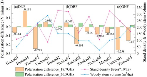
Table 3. Averaged polarization difference in transmissivity for different forest types with stand density and woody stem volume information.

Forest type	Averaged ρ (trees/ha)	Averaged Vol (m³/ha)	Averaged PD (γ(V) – γ(H))
			18.7 GHz	36.5 GHz
DNF	1718	156	–0.01	0.02
DBF	2393	97	–0.07	0.02
GNF	2102	165	–0.20	0.01

Mätzler (1994) noted that the influence of the polarization difference was quite small and could be ignored basing on ground-based microwave radiometer measurements on a deciduous broadleaf tree. Nevertheless, our observations suggest that for the forest type DNF and DBF, there are positive or negative polarization differences in γ at diverse sample plots, giving rise to an overall offsetting polarization difference that converges to zero. On the contrary, Kruopis et al. (1999) found that significant polarization differences in transmissivity at 18.7 GHz was observed for coniferous forests (GNF in this case), with γ for horizontally polarized waves smaller than vertically polarized waves. However, our results demonstrate that γ of GNF for horizontally polarized waves is obviously larger than that of vertically polarized ones, probably due to the dominant vertical orientation of coniferous needles (see photo GNF-1 in Figure 5). In conclusion, the polarization difference in transmissivity of different forest types, particularly GNF, needs to be considered in the process of modeling.

3.2. Empirical transmissivity model for diverse forest types

To explore the variations in γ for diverse forest types as a function of $Vol$, new models have been developed based on experimental observation data. The estimation of γ for each frequency and polarization with respect to the measured $Vol$ data is manifested in Figure 8. Following the work of Kruopis et al. (1999), γ can be linked to Vol in an exponential form for each frequency and polarization (p): (13) ${\gamma }^{f,p}=a_p+\left(1-a_p\right)\cdot \exp \left(-b_p\cdot Vol\right)$(13) where, $a_p$ and $b_p$ are empirical coefficients fitted by nonlinear least-squares regression. Parameter a characterizes the saturation value of γ of a very dense forest at a specific frequency. The values of (a, b) were optimized based on the minimum sum of the squared errors (SSE) of γ estimated through Eq. (7). The derived (a, b) coefficients with 95% confidence bounds and R² are demonstrated in Table 4 and Figure 8, respectively. By comparison, the predicted transmissivity with the model established by Kruopis et al. (1999) (abbreviated as Kruopis γ model) for the Finnish boreal forest are also plotted in Figure 8. As the nadir angle was 50° in Kruopis γ model, Eq. (8) was used for cosine angular correction to get the corresponding values of (a, b) at 55°. Note that the transmissivity values at 55° used in our fitted model were obtained by spline interpolation based on the actual observed data, rather than directly using Eq. (8).

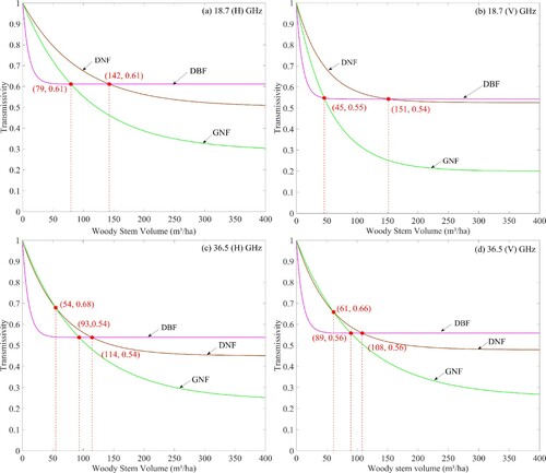
Figure 8. Retrieved transmissivity as a function of Vol for different forest types: (a) DNF, (b) DBF and, (c) GNF. The solid lines correspond to the optimized fitting models. Dashed line corresponds to the Kruopis γ model over its validity range (0–150 m³/ha), at 55° incidence angle. Values are referred to the fitted model. The red dots and lines refer to the vertical polarization, and the blue refers to the horizontal polarization.

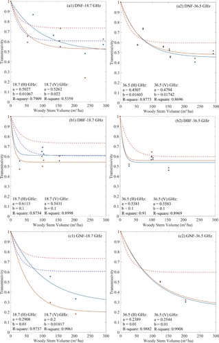
Table 4. Parameters in our γ model for each frequency and polarization at 55° incidence angle retrieved from curve-fitting on the measurements, shown in Figure 7 and compared to Kruopis γ model. (Note that the coefficients a and b in Kruopis γ model were obtained at an incidence angle of 55°.)

Forest Type	Frequency (polarization) GHz	Parameters in Kruopis γ model				Parameters in our γ model
		a	b	γs	Vols	a	b	γs	Vols
DNF	18.7 (H)	0.61	0.035	0.61	119	0.50	0.011	0.50	431
	18.7 (V)	0.74		0.74	102	0.53	0.022	0.53	205
	36.5 (H)	0.60*		0.60	120	0.45	0.016	0.45	300
	36.5 (V)	0.60		0.60	120	0.48	0.017	0.48	269
DBF	18.7 (H)	0.61	0.035	0.61	119	0.61	0.100	0.61	42
	18.7 (V)	0.74		0.74	102	0.54	0.100	0.54	44
	36.5 (H)	0.60*		0.60	120	0.54	0.100	0.54	45
	36.5 (V)	0.60		0.60	120	0.56	0.100	0.56	44
GNF	18.7 (H)	0.61	0.035	0.61	119	0.29	0.010	0.29	550
	18.7 (V)	0.74		0.74	102	0.20	0.018	0.20	330
	36.5 (H)	0.60*		0.60	120	0.24	0.010	0.24	576
	36.5 (V)	0.60		0.60	120	0.25	0.010	0.25	568

The newly developed γ models (abbreviated as our γ model) show that there is a series of specific relations for diverse forest types between γ and Vol at each frequency/polarization. As we expected, γ decreases as Vol increases until it reaches saturation. The transmissivity saturates for the reason that the forest canopy never covers 100% of the area, even though the forest cover is claimed to be 100%, as per the growth rules of vegetation. If we assume that the precision requirement of γ is 0.01, the saturation levels of γ (γ_s) and their corresponding saturation levels of Vol (Vol_s) can be calculated (see Table 4).

Our γ model manifests that: (1) γ for horizontal polarization is evidently higher than that for vertical polarization for all three forest types at 18.7 GHz, whereas it turns out to be slightly lower at 36.5 GHz. (2) γ saturates at higher Vol values for DNF (Vol_s values range from 205 to 431 m³/ha) and GNF (Vol_s values range from 330 to 576 m³/ha) than those suggested by the Kruopis γ model (Vol_s values range from 102 to 120 m³/ha), except for DBF (Vol_s values range from 42 to 45 m³/ha). Specifically, γ_s for DBF is 0.61, 0.54, 0.54, and 0.56 at 18.7 (H)-, 18.7 (V)-, 36.5 (H)-, and 36.5 (V)-GHz, respectively. These values could be used as the transmissivities at the above frequencies and polarizations for the majority of the DBF in China, considering that the average growing stock in forest land in China is 67 m³/ha (http://www.fao.org/forestry/32042/en/). (3) For high $Vol$ (> 120 m³/ha), the values of γ are generally smaller than those predicted by Kruopis γ model. Besides, evidently lower saturation levels of γ for GNF, compared with those in the Kruopis γ model, can also be found. The difference in γ variation characteristics between the Kruopis γ model and our γ model can be explained by the variability in tree species which have been investigated, the range of canopy structural characteristics, and experimental approach (e.g. radiometer loading platform, measurement scale). Nevertheless, the values of (a, b) in our γ model are approximately in agreement with the range proposed by (Langlois et al. 2011) and (Pardé, Royer, and Vachon 2005) after angular correction (Eq. (8)). However, their transmissivity models ignored the dependence of transmissivity on forest type. Even though it is limited by the sample size, the newly defined transmissivity model form and parameter range are basically consistent with the corresponding forest type in the previous studies as mentioned above.

Figure 9 indicates the variation of γ against Vol for three forest types at the same frequency and polarization in the newly developed transmissivity model. The red asterisks indicate the intersection points between the fitted curves, and the values in parentheses correspond to the Vol and γ, respectively. From the data shown in Figure 9, we can find out that: (1) Of the three forest types, the values of γ are in an order of DBF > DNF > GNF when their Vol exceeds 142, 151, 114 and 108 m³/ha for 18.7 (H)-, 18.7 (V)-, 36.5 (H)-, and 36.5 (V)-GHz, respectively. In addition, the values of γ for DNF are significantly lower than those for the other two forest types in the low volume range (See Table 1 and Table 4). This is due to the fact that sample plots represented by DNF are usually characterized by low Vol and high stand density in our study. (2) The variations of γ for DNF and GNF are almost identical when their Vol is in the range of 0–60 m³/ha, for 36.5 GHz. And when their Vol exceeds 61 m³/ha, values of γ for DNF remains higher than that of GNF. The reason for this significant difference on the values of γ is that the presence of needle-leaves on GNF increases scattering and leads to strong attenuation on microwave radiation. (3) A phenomenon should be noticed that γ for GNF is obviously lower at 36.5 (V) GHz than that at 18.7 (V) GHz (See also Figure 8), which seems to be ‘unreasonable’. We speculate that it may be related to the vertical distribution of canopy needles at an incidence angle of 55 degrees (See Figure 5, GNF-1). The above analysis indicates that the extreme complexity of the radiative transfer process in forest systems still requires more experiments to verify.

Figure 9. Variation of transmissivity retrieved by our γ model against Vol for three forest types at the same frequency and polarization.

3.3. Forward model simulation results

To evaluate the performance of the newly developed transmissivity model, the forward model has been applied to simulate $T_{B,sat}$ at the AMSR-2-pixel scale. Kruopis γ model and our γ model were incorporated into the forward model suite, with two kinds of extinction coefficients, respectively. A comparison of the simulated results was illustrated in Figure 10(a) and Table 5(a) with ${\kappa }_{e\mathrm{\_}Hallikainen}$, and in Figure 10(b) and Table 5(b) with ${\kappa }_{e\mathrm{\_}Roy}$ used. For the case where ${\kappa }_{e\mathrm{\_}Hallikainen}$ is used, it can be found that simulations using our γ model resulted in better performance, with a root-mean-square error (RMSE) of 6.4 K, 3.4 K, 8.6 K, and 7.9 K for 18.7 (H)-, 18.7 (V)-, 36.5 (H)-, and 36.5 (V)-GHz, respectively. Comparing with Kruopis γ model, it can be inferred that our γ model performed the best at 18.7 (V) GHz in DNF, with an RMSE reduction of 54%, and the overall improvement in accuracy averages 27% for DNF, –4% for DBF, and 19% for GNF, respectively. However, for the case of ${\kappa }_{e\mathrm{\_}Roy}$ being used, the simulated accuracy at 36.5GHz is significantly improved compared with the former case, while the simulated error at 18.7GHz is substantially increased for both Kruopis γ model and our γ model. Nevertheless, the overall simulated results of our γ model are still marginally better. Therefore, the newly developed transmissivity models are suitable for being incorporated into the forward model for simulating the satellite T_B. Furthermore, we can also draw the conclusion that it is a good approach to simulate the satellite T_B with high accuracy (∼3–6 K) to adopt ${\kappa }_{e\mathrm{\_}Hallikainen}$ for 18.7 GHz and ${\kappa }_{e\mathrm{\_}Roy}$ for 36.5GHz, separately.

Table 5(a). Comparison of the different transmissivity models with ${\kappa }_{e\mathrm{\_}Hallikainen}$ used to be incorporated into the forward model suite for simulation results against AMSR-2 T_B and the improvement in accuracy.

	Simulation with Kruopis γ model				Simulation with our γ model				Improvement in accuracy (%)
	18.7 (H)	18.7 (V)	36.5 (H)	36.5 (V)	18.7 (H)	18.7 (V)	36.5 (H)	36.5 (V)	18.7 (H)	18.7 (V)	36.5 (H)	36.5 (V)
DNF	6.9	6.3	10.3	7.6	7.1	2.9	7.3	5.8	−2	54	30	25
DBF	4.0	2.0	9.4	9.8	4.0	2.3	9.6	9.9	0	−13	−2	−2
GNF	9.5	7.0	14.3	11.3	8.5	6.3	10.5	8.8	11	10	27	22
Avg.	6.5	5.3	10.7	9.0	6.4	3.4	8.6	7.9	2	36	19	12

Figure 10. (a) Simulated results with ${\kappa }_{e\mathrm{\_}Hallikainen}$ used against AMSR-2 T_B. (b) Simulated results with ${\kappa }_{e\mathrm{\_}Roy}$ used against AMSR-2 T_B.

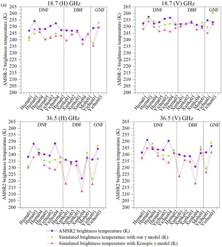
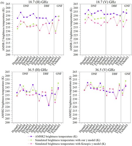
Table 5(b). Same as Table 5(a), except that the extinction coefficients were changed to ${\kappa }_{e\mathrm{\_}Roy}$.

	Simulation with Kruopis γ model				Simulation with our γ model				Improvement in accuracy (%)
	18.7 (H)	18.7 (V)	36.5 (H)	36.5 (V)	18.7 (H)	18.7 (V)	36.5 (H)	36.5 (V)	18.7 (H)	18.7 (V)	36.5 (H)	36.5 (V)
DNF	11.9	12.8	6.4	4.3	12.1	7.2	4.7	4.1	−2	42	26	4
DBF	10.6	9.0	5.1	4.7	10.5	8.5	5.7	5.2	0	6	−12	−10
GNF	15.4	14.8	7.6	4.7	13.2	9.2	6.7	5.6	14	37	12	−20
Avg.	12.0	11.9	6.1	4.5	11.8	8.0	5.4	4.8	2	32	12	−6

4. Discussion

Ground-based radiometric measurements, one of the cornerstones for obtaining new discoveries and conclusions, has made great progress in radiative transfer processes and improved model parameterization. The newly established transmissivity models based on radiation experiments have been proven to perform excellent in the T_B forward model simulation. Nonetheless, the ground-based observational experiment is far more complicated due to certain possible sources of error and uncertainties. One of the error sources is related to $T_{B,veg,\downarrow }$ as the tree canopy gaps and antenna pointing angles may cause some variations in the observation process. Besides, the effect of $T_{B,sky}$ on the calculation process should be taken into consideration.

4.1. Uncertainty on $T_{B,veg,\downarrow }$ caused by observation angles in ground-based radiometric measurements

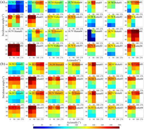
During the ground-based radiometric measurements, radiometers were used to observe the canopy T_B in multiple azimuths and incidence angles. The results for $T_{B,veg,\downarrow }$ with diverse combinations of azimuth and incidence angle are presented in Figure 11. The blank grid area in Figure 11 indicates that the observation at this azimuth/incidence angle was not implemented because of time constraints and harsh field conditions. The full dark blue grid area signifies that its values are negative and invalid. And the sample plots Huma01 and Huma04 missed data at 18.7 (V) GHz. Figure 11 demonstrates that $T_{B,veg,\downarrow }$ generally tends to increase with the incidence angle, and the variation of $T_{B,veg,\downarrow }$ at 36.5 GHz manifests more uniform numerical information compared with that at 18.7 GHz.

Figure 11. $T_{B,veg,\downarrow }$ observed on multiple incidence angles and azimuths at (a) 18.7- and (b) 36.5-GHz, H and V polarizations.

Table 6 summarizes the standard deviation (Std) of the measured $T_{B,veg,\downarrow }$ values from all samples in both cases. Case 1 refers to measurements performed at the same incidence angle but at different azimuths; Case 2 refers to measurements performed at the same azimuth but at different incidence angles. Std caused by azimuthal measurements (Case 1) averages 12 K and 9 K at 18.7- and 36.5-GHz, respectively. Correspondingly, Std caused by a 10° interval in incidence angle (Case 2) is approximately 20 K on an average with little distinction at each frequency/polarization. The estimations of γ and the error-bar shadows indicating Std of γ are presented in Figure 12. As the error bars in Figure 12 (a) and (b) shown, Std of γ induced by Case 1 at a fixed incidence angle of 50° ranges from 0.001–0.131, with an average of 0.040. For comparison, the measured multi-azimuthal $T_{B,veg,\downarrow }$ data with minimum Std among the three incidence angles (40°,50°, and 60°) over Case 2 was averaged. Then, the averaged $T_{B,veg,\downarrow }$ date at multiple incidence angle was substituted into Eq. (7) and Eq. (8) to retrieve γ at a unified incidence angle of 55°. Std of γ ranges from 0.001–0.084, with an average of 0.028, as demonstrated in Figure 12 (c) and (d). The variability on Std of γ was deemed to be due to the temporal variations of the radiometric signal during the measurement periods and possibly to more pronounced heterogeneity. Compared with previous research results (Pardé, Royer, and Vachon 2005; Langlois et al. 2011), the variability of γ retrieved from the radiometric measurements in this study was relatively smaller.

Figure 12. Estimations of the transmissivity with error bars in Case 1 at a fixed incidence angle of 50°: (a) 18.7 GHz and (b) 36.5 GHz; and Case 2 at a unified incidence angle of 55°: (c) 18.7 GHz and (d) 36.5 GHz.

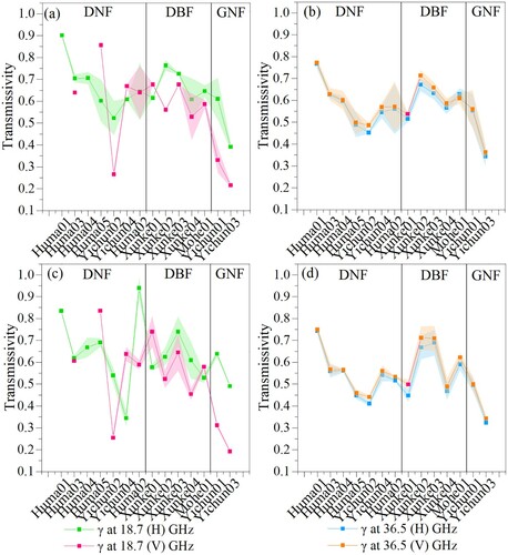
Table 6. Std of $T_{B,veg,\downarrow }$ from all sample plots at multi- azimuth and incidence angles for each frequency and polarization.

Frequency (polarization) GHz	Case 1: Different azimuths at the same incidence angle				Case 2: Different incidence angles at the same azimuth angle
	60°	50°	40°	mean	0°	90°	180°	270°	mean
18.7 (H)	12 ± 10	12 ± 10	14 ± 10	13	20 ± 8	20 ± 8	23 ± 7	10 ± 6	20
18.7 (V)	11 ± 15	9 ± 10	13 ± 11	11	19 ± 9	21 ± 11	19 ± 3	12 ± 8	19
36.5 (H)	8 ± 7	9 ± 7	10 ± 8	9	21 ± 6	20 ± 6	21 ± 7	13 ± 2	20
36.5 (V)	9 ± 8	9 ± 7	10 ± 8	9	20 ± 6	19 ± 6	21 ± 7	12 ± 2	19

From a theoretical point of view, significant statistical robustness needs to be based on a vast number of measurements over a wide range of scanning angles (azimuth and zenith). Nevertheless, considering the time cost of field experiments and the stringent radiometric requirements in particular, we suggest that scanning observations of the forest canopy at multiple azimuths should be given priority over observations at multiple incident zenith angles.

4.2. Deviation of measured transmissivity caused by $T_{B,sky}$

The $T_{B,veg,\downarrow }$ value can be expressed by Eq. (14) by substituting Eq. (6) into Eq. (5). Based on the RTE, we can obtain the following: (14) $T_{B,veg,\downarrow }=\gamma \cdot T_{B,sky}+(1-\gamma )\cdot (1-{\omega }_{veg})\cdot T_{veg}+r_{veg}\cdot T_{B,ground-r}$(14)

(15) $T_{B,ground-r}=k_T\cdot \left[e_G\cdot T_G+\left(1-e_G\right)\cdot k_T\cdot T_{B,veg,\downarrow }\right]$(15) (16) $k_T=\frac{\left(1-r_v\right)\left(1-r_G\right)}{{\left(1-\sqrt{r_v\cdot r_G}\right)}^2}$(16)

In this case, $k_T$ is the radiative transfer coefficient between the canopy and the ground surface, T_G is the physical temperature of the ground, and $e_G$ and $r_G$ are the emissivity and reflectivity of the ground surface, respectively.

According to the receiving principle of the microwave radiometer antenna, the effect of antenna sidelobe contribution needs to be taken into account, which is the main error source in ground-based measurements. In addition to the target T_B received by the main beam of the antenna, the antenna apparent radiometric temperature $\left(T_{B,obs}\right)$ also contains other radiation received by the sidelobe (Song, Zhao, and Guan 2008): (17) $T_{B,obs}={\eta }_m\cdot T_{B,veg\text{£},\downarrow }+\left(1-{\eta }_m\right)\cdot T_{B,side}$(17) In above equation, ${\eta }_m$ is the antenna main-beam efficiency (${\eta }_m=0.8$in this study), and $T_{B,side}$ is the sidelobe contribution. Note that in Section 2.3.3, the values of $T_{B,veg,\downarrow }$ were considered to be equal to $T_{B,obs}$. The sidelobe contribution is related to the ambient physical temperature. Slight variation can be ignored by using an antenna with high main-beam efficiency under the condition of a small temperature change. Therefore, such an approximation $T_{B,side}=T_{B,ground-r}$ can be obtained in this case. From the above Eq. (15) and Eq. (17), we can conclude that (18) $T_{B,veg,\downarrow }=\frac{T_{B,obs}-k_T\cdot e_G\cdot T_G\left(1-{\eta }_m\right)}{\left[{\eta }_m+k_T^2\cdot \left(1-{\eta }_m\right)\cdot \left(1-e_G\right)\right]}$(18) Furthermore, combining Eq. (14) and Eq. (18), γ can be expressed as (19) $\gamma =\frac{\left\{{\displaystyle \frac{T_{B,\mathrm{o}\mathrm{b}\mathrm{s}}-k_T\cdot e_G\cdot T_G\left(1-{\eta }_m\right)}{\left[{\eta }_m+k_T^2\cdot \left(1-{\eta }_m\right)\cdot \left(1-e_G\right)\right]}-\frac{\left(1-{\omega }_{veg}\right)\cdot T_{veg}+r_{veg}\cdot k_T\cdot e_G\cdot T_G}{1-r_{veg}\cdot k_T^2\cdot \left(1-e_G\right)}}\right\}}{\left\{{\displaystyle \frac{\left[T_{B,sky}-\left(1-{\omega }_{veg}\right)\cdot T_{veg}\right]}{1-r_{veg}\cdot k_T^2\cdot \left(1-e_G\right)}}\right\}}$(19) Eq. (19) indicates that the parameters, ${\eta }_m$, ${\omega }_{veg}$, $r_{veg}$, $e_G$ and $T_{B,sky}$ are challenging to measure accurately, and they include the measurement uncertainty, which is the main factor affecting $\gamma$. And the deviation of $\gamma$ $\left(\mathrm{\Delta }\gamma \right)$ is (20) $\mathrm{\Delta }\gamma =\frac{\mathrm{\partial }\gamma }{\mathrm{\partial }{\eta }_m}\cdot \mathrm{\Delta }{\eta }_m+\frac{\mathrm{\partial }\gamma }{\mathrm{\partial }{\omega }_{veg}}\cdot \mathrm{\Delta }{\omega }_{veg}+\frac{\mathrm{\partial }\gamma }{\mathrm{\partial }{r}_{veg}}\cdot \mathrm{\Delta }{r}_{veg}+\frac{\mathrm{\partial }\gamma }{\mathrm{\partial }{e}_G}\cdot \mathrm{\Delta }{e}_G+\frac{\mathrm{\partial }\gamma }{\mathrm{\partial }{T}_{\mathrm{B},\mathrm{s}\mathrm{k}\mathrm{y}}}\cdot \mathrm{\Delta }{T}_{\mathrm{B},\mathrm{s}\mathrm{k}\mathrm{y}}$(20) To simplify the following equations, reasonable assumptions were proposed. The difference in the equivalent permittivity between forest and air is relatively small, and therefore, $r_{veg}$ is generally approximated to 0.1. The $e_G$ in winter is 0.92–0.93 at 18.7- and 36.5-GHz referring to the experimental observation data provided by Wu et al. (2017). Here we set $e_G=0.93$. Considering that $T_{veg}=T_G$, from Eq. (16), we can obtain k_T = 0.9968, and hence set k_T as 1. The experimental data obtained in this study presents that: $\begin{array}{rl}& T_{veg}\in [258K,264K];\\ & T_{B,sky}\in \left[8\mathrm{K},11K\right],T_{B,obs}\in \left[28\mathrm{K},208K\right],\mathrm{w}\mathrm{h}\mathrm{e}\mathrm{n}\mathrm{a}\mathrm{t}18.7\mathrm{G}\mathrm{H}\mathrm{z};\\ & T_{B,sky}\in \left[17\mathrm{K},21K\right],T_{B,obs}\in \left[74\mathrm{K},178K\right],\mathrm{w}\mathrm{h}\mathrm{e}\mathrm{n}\mathrm{a}\mathrm{t}36.5\mathrm{G}\mathrm{H}\mathrm{z};\end{array}$when the viewing angle was 50°.

The influence of ${\omega }_{veg}$ on $\mathrm{\Delta }\gamma$ can be ignored (Mätzler 1994; Langlois et al. 2011), therefore, ${\omega }_{veg}$ is set to 0. Besides, solving Eq. (19) by substituting the relevant assumed values, we can obtain: (21) $\gamma =\frac{0.993\cdot T_{B,obs}-0.86\cdot T_{veg}-0.0065\cdot {\eta }_m\cdot T_{veg}}{\left(0.93\cdot {\eta }_m+0.07\right)\cdot \left(T_{veg}-T_{B,sky}\right)}$(21) To investigate thoroughly the $\mathrm{\Delta }\gamma$ caused by $T_{B,sky}$, a limiting case can be assumed based on the experimental data of this study. The mean value of $T_{veg}$ was taken as 260 K for the sake of simplicity because of its limited range. Through Eq. (21), the largest uncertainty error of observation due to $T_{B,sky}$ can be obtained as following formulas: (22) $\gamma =\frac{range}{260-T_{B,sky}}=\left\{\begin{array}{cc}\frac{-22.6to-242.2}{260-T_{B,sky}},& \mathrm{w}\mathrm{h}\mathrm{e}\mathrm{n}\mathrm{a}\mathrm{t}18.7\mathrm{G}\mathrm{H}\mathrm{z}\\ \frac{-59.2to-186.1}{260-T_{B,sky}},& \mathrm{w}\mathrm{h}\mathrm{e}\mathrm{n}\mathrm{a}\mathrm{t}36.5\mathrm{G}\mathrm{H}\mathrm{z}\end{array}\right.$(22) Thus, (23) $\frac{\mathrm{\partial }\gamma }{\mathrm{\partial }{T}_{B,sky}}\cdot \mathrm{\Delta }{T}_{B,sky}=\frac{-range}{{\left(260-T_{B,sky}\right)}^2}\cdot \mathrm{\Delta }{T}_{B,sky}$(23) According to the above formulas, assuming that the accuracy requirement of $\mathrm{\Delta }\gamma$ caused by $T_{B,sky}$ is 0.01, the observation accuracy of $\mathrm{\Delta }{T}_{B,sky}$ should be 2.6–28.0 K (at 18.7-GHz) and 3.2–9.9 K (at 36.5-GHz), respectively. Therefore, the observation accuracy of $\mathrm{\Delta }{T}_{B,sky}$ should be at least better than 2.6 and 3.2 K at 18.7- and 36.5-GHz, respectively, for winter measurement when the mean forest physical temperature value $T_{veg}$ is approximately 260 K (–13 °C). As $T_{B,sky}$ values for this study were modeled by using the MPM model, the modeling accuracy needs to be taken into consideration. Shi et al. (2017) validated the atmospheric downward radiation over China using the MPM model and Mie theory through a series of on-site ground-based radiometer experiments in North China. Their results showed that the RMSE between the measured and simulated values were 1.6 and 9.5 K at 18.7- and 36.5-GHz, respectively. Therefore, the $T_{B,sky}$ obtained from MPM model in this study meets the accuracy requirement at 18.7 GHz (1.6 K VS 2.6 K), but not at 36.5 GHz (9.5 K VS 3.2 K). This reveals that the simulated results at 36.5GHz are more susceptible to the accuracy of simulated $T_{B,sky}$ compared to that at 18.7GHz.

In addition to the aspects discussed above, the experimental results of $\gamma$ will be influenced by the near-surface freeze/thaw state (Zhao et al. 2011, 2017) and other geometric conditions (Montpetit et al. 2013), for instance, the difference in height of trees, thickness of forest (from radiometer to edge of the forest), distance of radiometer to the nearest tree. Even though the observations on forest transmissivity are complex and challenging, we have found that the influence of the main factors discussed above on the transmissivity calculation based on radiometric measurements is relatively small. Thus, our observation results are relatively reliable and applicable. Besides, the measurement of forest transmissivity for diverse forest types at various sites may provide insights for passive microwave remote sensing of vegetation, soil, and snow in the future.

5. Conclusion

The main objective of this study is to explore the characteristics of forest transmissivity at 18.7- and 36.5-GHz (typically used frequencies for snow parameter retrieval algorithms) for multiple forest types during the snow season. Therefore, ground-based radiometric observations have been performed in several typical forested regions in Northeast China. Based on experimental data, a group of new forest transmissivity models have been developed for diverse forest types, depending on woody stem volume and frequency/polarization.

The observation results demonstrate that γ at a certain frequency/polarization differs from diverse forest types within the same Vol range. The newly established transmissivity model performed excellent, with the simulation RMSE of 6.4 K, 3.4 K, 8.6 K, and 7.9 K for 18.7 (H)-, 18.7 (V)-, 36.5 (H)-, and 36.5 (V)-GHz for the case of adopting the extinction coefficients suggested by (Hallikainen, Ulaby, and Van Deventer 1987), respectively. In addition, we noticed that (Hallikainen, Ulaby, and Van Deventer 1987)’s extinction coefficients are more applicable to the satellite T_B simulation at 18.7-GHz, while Roy et al. (2012)’s coefficients are more suitable for 36.5-GHz. The newly established transmissivity model also indicates that: 1) A relatively constant value of γ could be used for the majority of DBFs with Vol value above 45 m³/ha at the frequencies of 18.7- and 36.5-GHz. 2) Of the three forest types, the values of γ are in an order of DBF > DNF > GNF when their Vol exceeds 142, 151, 114 and 108 m³/ha for 18.7 (H)-, 18.7 (V)-, 36.5 (H)-, and 36.5 (V)-GHz, respectively. 3) Values of γ for DNF remains higher than that for GNF when their Vol exceeds 61 m³/ha. Furthermore, we suggest that scanning observations of the forest canopy at multiple azimuths should be given priority over observations at multiple incident zenith angles if the diurnal duration of the field experiment is very limited.

As the microwave radiative transfer process of the forest-snow coupling system is relatively complex, and there are numerous uncertainties in the observational experiments of forest radiation, more validation data is required to test the newly developed model in the follow-up. One of the challenges is the problem of transmissivity applied to mixed pixels. Therefore, the construction of a miniaturized microwave radiometer boarded on an unmanned aerial vehicle observation system for detecting T_B above the canopy is also a critical component for the next step.

Acknowledgements

The authors would like to gratefully thank the anonymous reviewers for their constructive and encouraging comments on this work.

Disclosure statement

No potential conflict of interest was reported by the author(s).

Additional information

Funding

This work was supported by National Natural Science Foundation of China: [Grant Number 41771400]; National Natural Science Foundation of China: [Grant Number 41871248]; Science and Technology Basic Resources Investigation Program of China ‘Investigation on snow characteristics and their distribution in China’ [Grant Number 2017FY100500].

Notes

(‘DBF’ = ‘Deciduous Broad-leaved Forest’, ‘DNF’ = ‘Deciduous Needle-leaved Forest’, ‘GNF’ = ‘Evergreen Needle-leaved Forest’).

* Note that Kruopis et al. (1999) did not estimate the transmissivity model at 36.5 (H) GHz; the constant a reported here for 36.5 (H) GHz was the same as that for 36.5 (V) GHz as suggested by Pulliainen, Grandell, and Hallikainen (1999).

References

- Barnett, T. P., J. C. Adam, and D. P. Lettenmaier. 2005. “Potential Impacts of a Warming Climate on Water Availability in Snow-Dominated Regions.” Nature 438: 303–309. doi:https://doi.org/10.1038/nature04141.
- Chang, A. T. C., J. L. Foster, and D. K. Hall. 1996. “Effects of Forest on the Snow Parameters Derived from Microwave Measurements During the BOREAS Winter Field Campaign.” Hydrological Processes 10 (12): 1565–1574. doi:https://doi.org/10.1002/(SICI)1099-1085(199612)10:12 < 1565::AID-HYP501 > 3.0.CO;2-5.
- Cohen, Juval, Juha Lemmetyinen, Jouni Pulliainen, Kirsikka Heinilä, Francesco Montomoli, Jaakko Seppänen, and Martti Hallikainen. 2015. “The Effect of Boreal Forest Canopy in Satellite Snow Mapping—A Multisensor Analysis.” IEEE Transactions on Geoscience and Remote Sensing 53 (12): 6593–6607. doi:https://doi.org/10.1109/TGRS.2015.2444422.
- Derksen, Chris. 2008. “The Contribution of AMSR-E 18.7 and 10.7 GHz Measurements to Improved Boreal Forest Snow Water Equivalent Retrievals.” Remote Sensing of Environment 112 (5): 2701–2710. doi:https://doi.org/10.1016/j.rse.2008.01.001.
- Derksen, C., J. Strapp, A. Walker, J. Lemmetyinen, M. Hallikainen, and J. Pulliainen. 2009. “A Comparison of Airborne Microwave Brightness Temperatures and Snowpack Properties Across the Boreal Forests of Finland and Western Canada.” IEEE Transactions on Geoscience and Remote Sensing 47 (3): 965–978. doi:https://doi.org/10.1109/TGRS.2008.2006358.
- Derksen, C., A. Walker, and B. Goodison. 2003. “A Comparison of 18 Winter Seasons of In Situ and Passive Microwave-Derived Snow Water Equivalent Estimates in Western Canada.” Remote Sensing of Environment 88 (3): 271–282. doi:https://doi.org/10.1016/j.rse.2003.07.003.
- Derksen, C., A. Walker, and B. Goodison. 2005. “Evaluation of Passive Microwave Snow Water Equivalent Retrievals Across the Boreal Forest/Tundra Transition of Western Canada.” Remote Sensing of Environment 96 (3–4): 315–327.
- Ferrazzoli, P., L. Guerriero, and J.-P. Wigneron. 2002. “Simulating L-Band Emission of Forests in View of Future Satellite Applications.” IEEE Transactions on Geoscience and Remote Sensing 40 (12): 2700–2708. doi:https://doi.org/10.1109/TGRS.2002.807577.
- Foster, J. L., A. T. C. Chang, D. K. Hall, and A. Rango. 1991. “Derivation of Snow Water Equivalent in Boreal Forests Using Microwave Radiometry.” Arctic 44: 147–152. doi:https://doi.org/10.14430/arctic1581.
- Foster, James L., Chaojiao Sun, Jeffrey P. Walker, Richard Kelly, Alfred Chang, Jiarui Dong, and Hugh Powell. 2005. “Quantifying the Uncertainty in Passive Microwave Snow Water Equivalent Observations.” Remote Sensing of Environment 94 (2): 187–203. doi:https://doi.org/10.1016/j.rse.2004.09.012.
- Goodison, B. E., and A. E. Walker. 2020. “Canadian Development and Use of Snow Cover Information from Passive Microwave Satellite Data.” In Passive Microwave Remote Sensing of Land-Atmosphere Interactions, edited by B. J. Choudhury, E. G. Njoku, P. Pampaloni, and Y. H. Kerr, 245–262. Berlin: De Gruyte. doi:https://doi.org/10.1515/9783112319307-015.
- Groisman, Pavel Ya, Thomas R. Karl, and Richard W. Knight. 1994. “Observed Impact of Snow Cover on the Heat Balance and the Rise of Continental Spring Temperatures.” Science 263 (5144): 198–200. doi:https://doi.org/10.1126/science.263.5144.198.
- Hall, D. K., J. L. Foster, and A. T. C. Chang. 1982. “Measurement and Modeling of Microwave Emission from Forested Snowfields in Michigan.” Hydrology Research 13 (3): 129–138. doi:https://doi.org/10.2166/nh.1982.0011.
- Hallikainen, Martti T., Fawwaz T. Ulaby, and Tahera Emille Van Deventer. 1987. “Extinction Behavior of Dry Snow in the 18-to 90-GHz Range.” IEEE Transactions on Geoscience and Remote Sensing 6: 737–745. doi:https://doi.org/10.1109/TGRS.1987.289743.
- Kontu, Anna, and Jouni Pulliainen. 2010. “Simulation of Spaceborne Microwave Radiometer Measurements of Snow Cover Using In Situ Data and Brightness Temperature Modeling.” IEEE Transactions on Geoscience and Remote Sensing 48 (3): 1031–1044. doi:https://doi.org/10.1109/TGRS.2009.2030499.
- Kruopis, N., J. Praks, A. Arslan, H. Alasalmi, J. Koskinen, and M. Hallikainen. 1999. “Passive Microwave Measurements of Snow-Covered Forest Areas in EMAC’95.” IEEE Transactions on Geoscience and Remote Sensing 37 (6): 2699–2705. doi:https://doi.org/10.1109/36.803417.
- Kurum, Mehmet, Roger H. Lang, Peggy E. O’Neill, Alicia T. Joseph, Thomas J. Jackson, and Michael H. Cosh. 2011. “A First-Order Radiative Transfer Model for Microwave Radiometry of Forest Canopies at L-Band.” IEEE Transactions on Geoscience and Remote Sensing 49 (9): 3167–3179. doi:https://doi.org/10.1109/TGRS.2010.2091139.
- Langlois, Alexandre, Alain Royer, Florent Dupont, Alexandre Roy, Kalifa Goita, and G. Picard. 2011. “Improved Corrections of Forest Effects on Passive Microwave Satellite Remote Sensing of Snow Over Boreal and Subarctic Regions.” IEEE Transactions on Geoscience and Remote Sensing 49 (10): 3824–3837. doi:https://doi.org/10.1109/TGRS.2011.2138145.
- Langlois, A., A. Royer, and K. Goïta. 2010. “Analysis of Simulated and Spaceborne Passive Microwave Brightness Temperatures Using In Situ Measurements of Snow and Vegetation Properties.” Canadian Journal of Remote Sensing 36 (sup1): S135–S148. doi:https://doi.org/10.5589/m10-016.
- Larue, Fanny, Alain Royer, Danielle De Sèvec, Alexandre Langlois, Alexandre Roy, and Ludovic Bruckerde. 2017. “Validation of GlobSnow-2 Snow Water Equivalent Over Eastern Canada.” Remote Sensing of Environment 194: 264–277. doi:https://doi.org/10.1016/j.rse.2017.03.027.
- Li, Qinghuan, Richard Kelly, Juha Lemmetyinen, and Jinmei Pan. 2020. “Simulating the Influence of Temperature on Microwave Transmissivity of Trees During Winter Observed by Spaceborne Microwave Radiometery.” IEEE Journal of Selected Topics in Applied Earth Observations and Remote Sensing 13: 4816–4824. doi:https://doi.org/10.1109/JSTARS.2020.3017618.
- Li, Qinghuan, Richard Kelly, Leena Leppänen, Juho Vehviläinen, Anna Kontu, Juha Lemmetyinen, and Jouni Pulliainen. 2019. “The Influence of Thermal Properties and Canopy-Intercepted Snow on Passive Microwave Transmissivity of a Scots Pine.” IEEE Transactions on Geoscience and Remote Sensing 57 (8): 5424–5433. doi:https://doi.org/10.1109/TGRS.2019.2899345.
- Liebe, Hans J. 1989. “MPM—An Atmospheric Millimeter-Wave Propagation Model.” International Journal of Infrared and Millimeter Waves 10 (6): 631–650. doi:https://doi.org/10.1007/BF01009565.
- Liebe, Hans J., George A. Hufford, and Takeshi Manabe. 1991. “A Model for the Complex Permittivity of Water at Frequencies Below 1 THz.” International Journal of Infrared and Millimeter Waves 12 (7): 659–675. doi:https://doi.org/10.1007/BF01008897.
- Lin, Chang–Geng. 1964. “The Problem of Stem Shape Control in Forest Stock Measurement Techniques.” [in Chinese] Forestry Science 9 (4): 365–375.
- Mätzler, Christian. 1987. “Applications of the Interaction of Microwaves with the Natural Snow Cover.” Remote Sensing Reviews 2 (2): 259–387. doi:https://doi.org/10.1080/02757258709532086.
- Mätzler, Christian. 1994. “Microwave Transmissivity of a Forest Canopy: Experiments Made with a Beech.” Remote Sensing of Environment 48 (2): 172–180. doi:https://doi.org/10.1016/0034-4257(94)90139-2.
- Mätzler, Christian. 2006. Thermal Microwave Radiation: Applications for Remote Sensing. London: Institution of Engineering and Technology. doi:https://doi.org/10.1049/PBEW052E.
- Mo, T., B. Choudhury, T. Schmugge, James R. Wang, and T. Jackson. 1982. “A Model for Microwave Emission from Vegetation-Covered Fields.” Journal of Geophysical Research 87: 11229–11237. doi:https://doi.org/10.1029/JC087iC13p11229.
- Montpetit, Benoit, Alain Royer, Alexandra Roy, Alexandra Langlois, and Chris Derksen. 2013. “Snow Microwave Emission Modeling of Ice Lenses Within a Snowpack Using the Microwave Emission Model for Layered Snowpacks.” IEEE Transactions on Geoscience and Remote Sensing 51 (9): 4705–4717. doi:https://doi.org/10.1109/TGRS.2013.2250509.
- Pampaloni, Paolo. 2004. “Microwave Radiometry of Forests.” Waves in Random Media 14 (2): S275–S298. doi:https://doi.org/10.1088/0959-7174/14/2/009.
- Pardé, K. Goita, A. Royer, and F. Vachon. 2005. “Boreal Forest Transmissivity in the Microwave Domain Using Ground-Based Measurements.” IEEE Geoscience and Remote Sensing Letters 2 (2): 169–171. doi:https://doi.org/10.1109/LGRS.2004.842469.
- Pellarin, T., J.-P. Wigneron, J.-C. Calvet, M. Berger, H. Douville, P. Ferrazzoli, Y. H. Kerr, et al. 2003. “Two-year Global Simulation of L-Band Brightness Temperatures Over Land.” IEEE Transactions on Geoscience and Remote Sensing 41 (9): 2135–2139. doi:https://doi.org/10.1109/TGRS.2003.815417.
- Pulliainen, J. T., J. Grandell, and M. T. Hallikainen. 1999. “HUT Snow Emission Model and its Applicability to Snow Water Equivalent Retrieval.” IEEE Transactions on Geoscience and Remote Sensing 37 (3): 1378–1390. doi:https://doi.org/10.1109/36.763302.
- Roy, Vincent, Kalifa Goïta, Alain Royer, Anne E. Walker, and Barry E. Goodison. 2004. “Snow Water Equivalent Retrieval in a Canadian Boreal Environment from Microwave Measurements Using the HUT Snow Emission Model.” IEEE Transactions on Geoscience and Remote Sensing 42 (9): 1850–1859. doi:https://doi.org/10.1109/TGRS.2004.832245.
- Roy, Alexandre, Alain Royer, Jean-Pierre Wigneron, Alexandre Langlois, Jean Bergeron, and Patrick Cliche. 2012. “A Simple Parameterization for a Boreal Forest Radiative Transfer Model at Microwave Frequencies.” Remote Sensing of Environment 124: 371–383. doi:https://doi.org/10.1016/j.rse.2012.05.020.
- Shi, Lijuan, Yubao Qiu, Jiancheng Shi, Juha Lemmetyinen, and Shaojie Zhao. 2017. “Estimation of Microwave Atmospheric Transmittance Over China.” IEEE Geoscience and Remote Sensing Letters 14 (12): 2210–2214. doi:https://doi.org/10.1109/LGRS.2017.2756111.
- Song, Dongsheng, Kai Zhao, and Zhi Guan. 2008. “Tipping Calibration for Digital Gain Compensative Microwave Radiometer and Correction on Antenna Sidelobe Influences.” Radio Science 43 (4). doi:https://doi.org/10.1029/2007RS003679.
- Tait, A. B. 1998. “Estimation of Snow Water Equivalent Using Passive Microwave Radiation Data.” Remote Sensing of Environment 64 (3): 286–291. doi:https://doi.org/10.1016/S0034-4257(98)00005-4.
- Tedesco, Marco, and Parag S. Narvekar. 2010. “Assessment of the NASA AMSR-E SWE Product.” IEEE Journal of Selected Topics in Applied Earth Observations and Remote Sensing 3 (1): 141–159. doi:https://doi.org/10.1109/JSTARS.2010.2040462.
- Ulaby, Fawwaz Tayssir, Richard K. Moore, and Adrian K. Fung. 1986. Microwave Remote Sensing: Active and Passive. Volume 3-from Theory to Applications. Reading, Mass: Addison –Wesley Publishing Company.
- Vander Jagt, B. J., M. T. Durand, S. A. Margulis, E. J. Kim, and N. P. Molotch. 2015. “On the Characterization of Vegetation Transmissivity Using LAI for Application in Passive Microwave Remote Sensing of Snowpack.” Remote Sensing of Environment 156: 310–321. doi:https://doi.org/10.1016/j.rse.2014.09.001.
- Wegmuller, U., and C. Mätzler. 1999. “Rough Bare Soil Reflectivity Model.” IEEE Transactions on Geoscience and Remote Sensing 37 (3): 1391–1395. doi:https://doi.org/10.1109/36.763303.
- Wu, Lili, Xiaofeng Li, Kai Zhao, and Xingming Zheng. 2017. “Snow Depth Inversion Using the Localized HUT Model Based on FY-3B MWRI Data in the Farmland of Heilongjiang Province, China.” Journal of the Indian Society of Remote Sensing 45 (1): 89–100. doi:https://doi.org/10.1007/s12524-016-0578-1.
- Zhang, Lei, Kun Jia, Xiaosong Li, Quanzhi Yuan, and Xinfeng Zhao. 2014. “Multi-scale Segmentation Approach for Object-Based Land-Cover Classification Using High-Resolution Imagery.” Remote Sensing Letters 5 (1): 73–82. doi:https://doi.org/10.1080/2150704X.2013.875235.
- Zhao, Tianjie, Jiancheng Shi, Tongxi Hu, Lin Zhao, Defu Zou, Tianxing Wang, Dabin Ji, Rui Li, and Pingkai Wang. 2017. “Estimation of High-Resolution Near-Surface Freeze/Thaw State by the Integration of Microwave and Thermal Infrared Remote Sensing Data on the Tibetan Plateau.” Earth and Space Science 4 (8): 472–484. doi:https://doi.org/10.1002/2017EA000277.
- Zhao, Tianjie, Lixin Zhang, Lingmei Jiang, Shaojie Zhao, Linna Chai, and Rui Jin. 2011. “A New Soil Freeze/Thaw Discriminant Algorithm Using AMSR-E Passive Microwave Imagery.” Hydrological Processes 25 (11): 1704–1716. doi:https://doi.org/10.1002/hyp.7930.