Latitudinal fluctuation in global concentration of CO₂ and CH₄ from shortwave infrared spectral observation by GOSAT during COVID-19

ABSTRACT

Various countries have rapidly implemented strict actions to slow the blowout of COVID-19. Many events were dis-regarded, and anthropogenic activities such as industrial and transport systems were at a stoppage. Many countries were on lockdown, including the largest emitters of carbon dioxide. Due to these lockdowns, anthropogenic activities have been reduced and reported that air quality improves at a regional scale in many countries, including India. Therefore, the current study using Greenhouse Gases Observing Satellite (GOSAT/IBUKI) datasets to monitor the fluctuation of the average global concentration of dry mole fractions of atmospheric Methane (CH₄) and Carbon Dioxide (CO₂) during these pandemic lockdowns from January to June 2020. Outputs emphasize no significant reduction in the average concentration of dry mole fractions of atmospheric CH₄ over the globe, but a minor reduction was observed in global CO₂ engagement. The average concentration of both gases compares at each ten-degree latitude. The study reveals that, against the regional breakdowns, these short time lockdowns are not enough to control the concentration of these greenhouse gases at a larger scale, such as 10˚ latitude and globally, except for a minor reduction in CO₂ concentration.

KEYWORDS:

• Lockdown
• pandemic
• air quality
• greenhouse gas
• methane
• carbon dioxide

1. Introduction

Climate change is a significant challenge for humanity. In recent years, international exertions have strengthened to struggle to reduce the dangers of climate change. At present, global warming is one of the most crucial and extensively studied matters. Specifically, the increase in CO₂ concentration in the atmosphere is due to anthropogenic activities blamed for global warming (Sun et al. 2020). The global concentration of CO₂ was 280 ppm before industrialization, but now it has increased more than 410 ppm (Mustafa et al. 2021). Managing climate change necessitates exact information of the global budget of atmospheric greenhouse gases (GHGs). Accurate information on the carbon budget on regional and global scales is essential to design mitigation strategies to control atmospheric GHGs emissions (Mustafa et al. 2020). Although, regional air pollution is a significant alarm than climate change in many developing countries. Therefore, environmental policies must be designed to decrease air pollutants and GHGs emissions (Takeshita 2012). Climate change policies have mainly intended to reduce GHG emissions with other positive benefits, generally called co-benefits (IPCC 2001; 2007; 2014). According to previous studies, human health co-benefits can be considerable by decreasing co-emitted air contaminants (West et al. 2013). A connection is accepted between regional air pollution mitigation and GHGs (IPCC 2007), in addition to co-benefits can have substantial influences on the climate policies for cost-effectiveness. If these co-benefits are combined with GHG mitigation policies, the budget for controlling regional air pollutants might be reduced (Shrestha and Pradhan 2010). To accomplish the goals of UNFCCC, emission reduction has been essential in both developed and developing countries to decline quickly. A significant contribution by developing countries may take numerous procedures. An expressive gift of developing countries may take various procedures. Sustainable development strategies and procedures may be an inspirational accomplishment for climate change mitigation (Winkler, Höhne, and Elzen 2008).

In this scenario, a new tactic is in the discussion, and many studies show that local or regional air quality is improving due to coronavirus disease 2019 (COVID-19) lockdowns. COVID-19 has already occupied pandemic magnitudes, affecting the whole globe in a matter of weeks. The blowout of COVID-19 is already overwhelming and has touched the essential epidemiological criteria to be confirmed a pandemic (Remuzzi and Remuzzi 2020). The U.S., Europe, and most countries in Asia have stopped hitting the snooze button; after almost two months of COVID-19 alarm, the blowout outbreak sounded more loudly. Many countries took sudden actions and implemented many strict measures to mitigate the spread of the pandemic. Schools, Universities, restaurants, bars, offices, clubs, industries, and transportations have been shut down in many countries. The gathering has been prohibited and ordered everyone to stay at home (Cohen and Kupferschmidt 2020). According to the pandemic dynamics, most countries applied partial or full lockdowns to mitigate the spread of COVID-19 (Alvarez, Argente, and Lippi 2020). Anthropogenic activities have been shut downed due to these lockdowns, and it is informed that regional air quality is improving due to these reduced anthropogenic activities. GHGs emission is directly linked to human activities in the power sector. During lockdowns, there was a sharp decline in the global emission of these pollutants by a fall in industrial activities and energy demand (Nguyen et al. 2021). Wang et al. (2020) stated that anthropogenic emission declines, mostly industrial and transportation, diminishes PM_2.5 concentrations. The reductions of PM_2.5 Concentration in Chinese cities such as Wuhan, Guangzhou, Beijing, and Shanghai were 30.79, 5.35, 9.23, and 6.37 μg/m3, respectively. Zangari et al. (2020) observed a 36% and 51% reduction in the Concentration of PM_2.5 and NO_2, respectively, after the lockdown in New York City. Berman and Ebisu (2020) state that NO₂ concentration was reduced during the COVID-19 period with a 25.5% decrease with an absolute reduction of 4.8 ppb. Mandal and Pal (2020) observed a clear reduction in PM₁₀ concentration after eighteen days of the beginning of lockdown in stone mines. They also observed that noise level and Land surface temperature (LST) also dropped, and adjacent Dwarka River (India) water quality also enhanced due to the shutdown of dust discharge to the river. A newspaper in India, namely New Indian Express, on April 24, 2020, stated that the water quality of river Ganga is enhanced by 40–50% because of COVID-19 lockdown. These are the clear indications that due to COVID-19 lockdowns, ambient air quality and river ecosystems improved rapidly. More studies have also revealed reductions in transportation-related air pollutant concentrations in some megacities such as Wuhan, Barcelona, and Sao Paulo during lockdowns (Cadotte 2020; Li et al. 2020; Tobías et al. 2020; Zheng et al. 2020). Lockdown took place in China, and carbon and NO₂ emissions decreased by 25% and 30%, respectively (Isaifan 2020). Recently, the effect of the increasing significance of international trade on CO₂ emission has been paid attention. The use of water, materials, land, and biodiversity pressures have been considered in this admiration. In carbon dioxide emission, maximum developed countries have become stable their demand in national emissions, but their national emissions have increased even more in developing countries. (Arto and Dietzenbacher 2014). The international prose has waged ample consideration to ‘fringe benefits’ of GHGs policies. The idea is that GHGs emission reduction will decrease regional air pollution in developing countries. Therefore, it is debated that it is possible to simultaneously improve regional air quality and reduce greenhouse gas emissions (Table 1). It is a policy agenda to tackle regional air quality first, and then GHGs are considered. (Gielen and Changhong 2001). Nowadays, due to human activities, increasing global temperature complements the increasing proportion of GHGs. Climate change is one of the main distresses of humanity, and the adverse effects of GHGs emissions on people's health cannot be ignored. Today, an unusual intensification in global temperature is a tribute to the increasing proportion of GHGs emissions due to human activities. CO₂, CH₄, water vapor (H₂O), ozone (O₃), and nitrous oxide (N₂O) are the most abundant GHGs in the atmosphere (Hosseini, Wahid, and Aghili 2013). Hence, this study was conducted to find out the global fluctuation of CH₄ and CO₂ concentration at every 10° latitude during the COVID-19 pandemic and compared with the monthly global average concentration of both gases from GOSAT distribution of the year 2019 and the global monthly average of both gases from the data of Global Monitoring Lab (National Oceanic and Atmospheric Administration) (NOAA/GML) data. GOSAT provides data from 70°N to 50°S latitudes covering almost all countries that were shut down during COVID-19. We compared the monthly global average dry mole fraction of CO₂ and CH₄ observed by GOSAT from January to June 2020.

Table 1. Regional studies from different countries with various parameters.

	Region of Study	Parameters	Effect of COVID19 (Reduction in percent or unit)	Citation
1	Ontario, Canada	PM2.5 NO2 NOx O3	0.1-0.3 µg/m3 0.3-3.1 ppb 0.1-4.4 ppb 0.6-2.5 ppb	(Adams 2020)
2	China	NO2 PM2·5	12.9 µg/m3 18.9 µg/m3	(Chen et al. 2020)
3	New York City	PM2.5 NO2	36% (8.98 µg/m3) 51% (20.6 ppb)	(Zangari et al. 2020)
4	Kolkata, India	PM10 PM2.5 SO2 NO2 CO	8.94-20.9% 16.02-20.04% 5.08-17.93% 8.04-15.19% 1.61-6.88%	(Bera et al. 2021)
5	United States	PM2.5 NO2	25.5% 5.5%, 26.0% (Urban)	(Berman and Ebisu 2020)
6	Dwarka river basin, India	PM10 (At different sites)	92.22 µg/m3 147.14 µg/m3 211.78 µg/m3 153.77 µg/m3	(Mandal and Pal 2020)
7	India	PM2.5 PM10 NO2 CO	40-60% 40-60% 30-70% 20-40%	(Singh et al. 2020)
8	India	Aerosol optical depth (AOD)	45%	(Ranjan, Patra, and Gorai 2020)
9	East China	NO2 CO	30% 20%	(Filonchyk et al. 2020)
10	Iran	NO2 SO2 CO PM10	1.33% 5-28% 5-41% 1.4-30%	(Broomandi et al. 2020)
11	Pittsburgh, U.S.	PM2.5 CO and NO2 at high traffic sites	̴ 3 µg/m3 50%	(Tanzer-Gruener et al. 2020)

2. Methodology

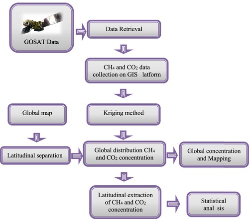
Greenhouse Gas Observing Satellites (GOSAT) can monitor the greenhouse gas concentration in continuous space and time, such as CO₂, CH₄, O_3, and water vapor. It was developed to retrieve total-column abundances of CH₄ and CO₂. The satellite's altitude is 666 km in a sun-synchronous orbit with 98˚ inclination that crosses the Equator at 12:49 local time. It observes column-averaged dry-air mole fraction of CH₄ and CO₂ with a footprint of 10.5 km² at nadir by Thermal and Near-Infrared Sensor for carbon Observation (TANSO)-Fourier Transform Spectrometer (FTS). Another sensor, namely TANSO–Cloud and Aerosol Imager (TANSO-CAI), is used to recognize aerosol and cloud data such as effective radius, optical thickness, cloud and aerosol properties, and existence by TANSO–FTS. Band number 3 and 4 of TANSO–FTS belongs to a strong water vapor absorption band and a thermal infrared band, respectively (Eguchi and Yoshida 2019; Sharma and Verma 2020; Mustafa et al. 2020; Belikov et al. 2021).

TANSO–FTS L3 spectral data used in this study to sense high-level clouds for the determination of decreasing the error in retrieved trace gases, such as column-averaged dry-air mole fractions of CH₄ (XCH₄) and CO₂ (XCO₂), which are also derived from the TANSO–FTS spectral data. GOSAT L3 datasets were downloaded from the website, and then the concentration of XCH₄ and XCO₂ was retrieved from the data using GOSAT HDF viewer Version 0.1.2.0 software. Spatial information of XCH₄ and XCO₂ was also recovered from the data.

Kriging method was applied for the spatial distribution of the concentration of XCH₄ and XCO₂. Data were collected from January 2020 to June 2020 (COVID-19 pandemic period). After the spatial distribution of these greenhouse gases, statistical analysis was done according to data availability and distribution (Figure 1). Results were compared with the datasets observed by Global Monitoring Laboratory (GML) of National Oceanic and Atmospheric Administration Monitoring (NOAA) and global CO₂ concentration compared with Mauna Loa, Hawaii ground station data. GML conducts research on three most important tasks: greenhouse gas and carbon cycle feedbacks, changes in clouds, aerosols, and surface radiation, and recovery of stratospheric ozone.

Figure 1. Methodology flow chart for the study.

2.1. Statistical analysis

Two types of statistical analysis were done: the non-parametric Mann Kendall (M.K.) test to analyze each variable's nonlinear increase or decrease trend. Secondly, Sen's slop to examine the slope of linear trends (Hernández-Paniagua et al. 2015). Mann Kendall's method does not necessitate the data to be normally distributed. According to M.K. analysis, the null hypothesis (H₀) is that the data series are identically distributed and independent. In contrast, the alternative hypothesis (H_.A.) is that the data series follows an increase or decrease monotonic trend (Uddin, Mishra, and Smyth 2020).

The Mann Kendall statistics S: (1) $S=\sum _{i=1}^{n-1}\sum _{k=i+1}^{n}sign(x_k-x_i)$(1) Where S is M.K. statistic, a sign is the signum function, $x_i$ and $x_k$ are time series. $x_i$ data is considered as a locus point and equated with remaining data points $x_k$ so that, (2) $S\mathrm{i}gn(x_k-x_i)=\left\{\begin{array}{c}1if(x_k-x_i)>0\\ 0if(x_k-x_i)=0\\ -1if(x_k-x_i)<0\end{array}\right\}$(2)

The positive value of Mann Kendall statistics (S) indicates an increasing trend, and the negative value indicates decreasing trend. The Statistic S can be Gaussian for n=18 with the variance (Var (s)) and mean E(s) = 0. The Var (S) is specified by: (3) $Var(S)={\displaystyle \frac{n(n-1)(2n-5)-{\sum }_{i-1}^m{t}_i(i)(i-1)(2i+5)}{18}}$(3) Where, $t_i$ is the number of tied groups.

Respectively, the standardized statistically significant trend is evaluated using standard statistic (Z) that delivers the final decision of the M.K. test. (4) $Z=\left\{\begin{array}{c}{\displaystyle \frac{s-1}{\sqrt{Var(S)}}ifS>0}\\ 0ifS=0\\ {\displaystyle \frac{s+1}{\sqrt{Var(S)}}ifS<0}\end{array}\right\}$(4) A positive output of standard statistic (Z) specifies an increasing trend, whereas a negative outcome specifies decreasing trend. A two-tailed test at the α level of significance is used to test an increasing or decreasing trend. (Patle et al. 2015; Meshram et al. 2018).

2.2. Sen's Slop Estimator

Thei-Sen's estimater further examined the degree of trend estimated by the M.K. test. The degree of trend is projected by Sen's slope estimator (Qi). (5) $(Q_i)=median\left({\displaystyle \frac{x_j-x_k}{j-k}}\right)fori=1,2,3,\dots ,N$(5) Where, $x_j\mathrm{and}{x}_k$ are outputs of data at time j and k, j > k, respectively.

A positive output of $Q_i$ shows an upward trend, and the negative output shows a downward trend (Patle et al. 2015; Meshram et al. 2018). Linear regression analysis was also performed to estimate the relationship of the trend of global CH₄ and CO₂.

3. Results and discussion

Linear regression, M.K. test analysis, and Sen's slope estimator were used to negotiate the monthly trends of CH₄ and CO₂. The statistical outputs enlisted using the Mann Kendall test of the monthly trend for both gases are shown in Table 2.

Table 2. Mann Kendall test statistics.

Mann-Kendall trend test / Two-tailed test
	Methane			Carbon dioxide
	2020	2019	NOAA	2020	2019	Mauna
Kendall's tau	0.8	0.8	−0.2	0.6	0.4	0.6
S	8	8	−2	6	4	6
Var(S)	16.66	16.66	16.66	16.66	16.66	16.66
p-value (Two-tailed)	0.08	0.08	0.80	0.22	0.46	0.22
alpha	0.05	0.05	0.05	0.05	0.05	0.05

Collectively a slight upward trend was observed of CH₄ in 2020, which is similar to the trend of the year 2019, and a trend was not significant at 0.05 confidence level. Figure 2a shows the atmospheric CH₄ concentration demonstrated a slight increase of 0.0202 ppt from January to June. Similarly, it shows the same trend in the year 2019. The linear relationships between global CH₄ Concentration of 2020, 2019 and ground station NOAA/GML were demonstrated in Figure 2a, in which R² is 0.8853, 0.875, and 0.0052, respectively. The mean and standard deviation (SD) of monthly global CH₄ are significantly different for 2020, 2019, and NOAA/GML data; the mean was 1.842, 1.834, and 1.874 ppt, where as SD was 0.008, 0.008, and 0.002, respectively. The linear trend lines of CH₄ in 2020 showed an upward trend similar to 2019 but slightly different from NOAA/GML data of the year 2020. In addition, the R² analysis displayed a poor relationship with NOAA/GML data but showed a strong relationship with global CH4 Concentration of 2019 by GOSAT data. Comparison of global CH₄ concentration results to the global concentration of CH₄ observed by NOAA/GML that shows a similar trend with 1.8731, 1.8731, 1.8752, 1.8765, 1.8747, and 1.8722 ppt for January, February, March, April, May, and June, respectively (Figure 2).

Figure 2. Monthly global Concentration of (a) CH₄ and (b) CO₂ during Jan-June (2019-2020).

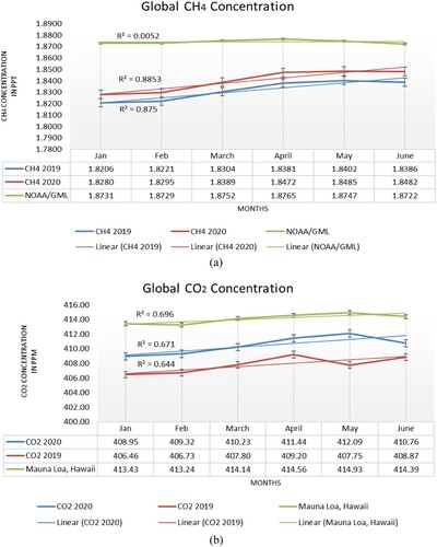
According to Sen's Slop Estimator (Table 3), the magnitude of trend (Qi) showed a positive output for 2020 with a 0.0047 slope value which offers a slightly upward trend. The slope value for the year 2019 also showed a positive direction with 0.0045, but NOAA/GML data showed a minor negative slope value with −0.0002, which is because of the data of June month. The overall global distribution of CH₄ is shown in Figure 3.

Table 3. Sen's slope statistics.

		Methane			Carbon dioxide
		Value	Lower bound (95%)	Upper bound (95%)	Value	Lower bound (95%)	Upper bound (95%)
2020	Slope	0.0047	0.0005	0.0088	0.7842	−0.3384	1.0584
	Intercept	1.82	1.81	1.84	407.88	407.05	412.79
2019	Slope	0.0045	0.0002	0.0079	0.4457	−0.1643	1.2319
	Intercept	1.81	1.80	1.83	406.19	404.09	408.56
NOAA (CH4)/ Mauna (CO2)	Slope	−0.0002	−0.0021	0.0018	0.3825	−0.085	0.66
	Intercept	1.87	1.86	1.88	412.99	411.92	414.9

On the other hand, overall, a slightly upward trend was found of CO₂ in 2020, which is similar to the trend of the year 2019, except and a trend was not significant at 0.05 confidence level. Figure 2b shows that CO₂ concentration demonstrated a slight increase of 1.81 ppm from January to June. Similarly, it shows the same trend with Mauna ground station data in 2020 and GOSAT data in the year 2019 also. The linear relationships between global CO₂ concentration of 2020, 2019, and Mauna ground station data were demonstrated in Figure 2b, in which R² is 0.696, 0.644, and 0.671, respectively. The mean and SD of monthly global CO₂ is significantly different for 2020, 2019, and Mauna station; the mean was 410.76, 408.07, and 414.25 ppm, where as SD was 1.071, 0.984, 0.634, respectively. The linear trend lines of CO₂ in 2020 showed an upward trend similar to 2019 and the ground station. In addition, the R² analysis exposed the exact relationship between the global CO₂ concentration of 2020 and the ground station. According to Mauna Loa, Hawaii ground station CO₂ concentration was 413.43, 413.24, 414.14, 414.56, 414.93 and 414.39 ppm for January, February, March, April, May, and June, respectively, which shows a similar trend of the year 2020 GOSAT data (Figure 2).

Figure 2a showed a decline of 1.33 ppm in June 2020 compared to May; similarly, Mauna station data also showed a slight decrease, which showed a reduction in global CO₂ concentration. Some studies also showed a drop in global CO₂ engagement. IEA 2020 report showed a 3.8% fall in worldwide energy demand leading to an over 5% reduction in CO₂ emission in the first quarter of 2019 (IEA 2020). In another study, a rapid 8.8% (−1551 Mt) reduction of global CO₂ was observed in the initial six months of 2020 compared to 2019 (Liu et al. 2020). These studies support the results of current study.

According to Sen's Slop Estimator (Table 3), the magnitude of trend (Qi) showed a positive output for the year 2020 with a 0.7842 slope value which shows an upward trend, and the slope value for the year 2019 and Mauna ground station data also showed a positive direction with 0.4457 and 0.3825, respectively. The overall global spatial distribution of CH₄ and CO₂ is shown in Figures 3 and 4, respectively.

Figure 3. Global spatial distribution of Methane.

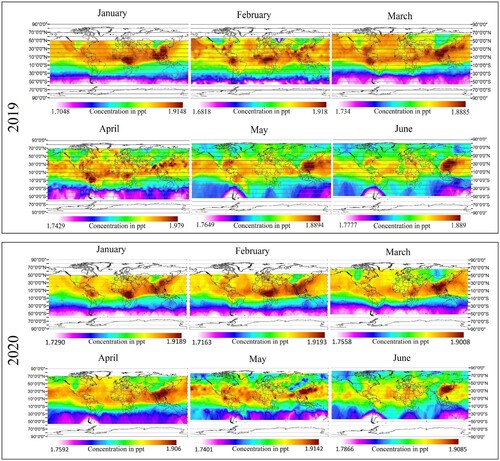
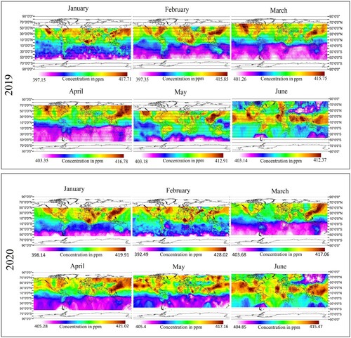
Figure 4. Global spatial distribution of Carbon dioxide.

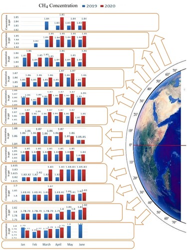
3.1. Latitudinal fluctuations in CH₄ concentration

Latitudinal distribution of Methane from January-June 2020 was compared with 2019 for the same months on a ten-degree basis from 70˚N to 50˚S on the global scale (Figure 5). In the northern hemisphere, the mean concentration of CH₄ of June month showed a minor reduction on 0˚N to 30˚ N and 60˚N to 70˚N latitudes with 0.01 ppt. In contrast, the same concentration was observed on 30˚N to 60˚N latitude compared to the mean concentration of January month, but the same trend was observed with a mean concentration of CH₄ of the year 2019. On the other hand, in the southern hemisphere, mean concentration reduced on 0˚S to 10˚S latitude but on other latitudes from 10˚S to 50˚S, it increased continuously, and a similar trend was observed in 2019 also.

Figure 5. Monthly latitudinal distribution of CH₄ for the years 2019 and 2020.

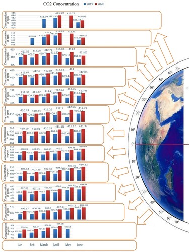
3.2. Latitudinal fluctuations in CO₂ concentration

The latitudinal distribution of CO₂ from January-June 2020 was compared with the year of 2019 for the same months on a ten-degree basis from 70˚N to 50˚S on a global scale (Figure 6). According to the distribution of CO₂ in the northern hemisphere, it is observed that the concentration was continuously increasing from 0˚ to 40˚N and decreasing from 40 ˚ to 70 ˚N if it is compared with the mean CO₂ concentration of January. The results showed that CO₂ reduced in the northern hemisphere in June compared to May 2020 from 10˚-70˚N latitude. In 2019, on 10˚ to 40˚N, the mean CO₂ concentration in June showed an increase compared to May. But in 2020, it showed a minor reduction that should be noticeable because most lockdown countries are in the same latitudinal zone. According to a study (Liu et al. 2020)., significant reductions were observed in the E.U. 27 & U.K. by 19.3%, India by 12.7%, and the U.S. by 7.6%, compared to a slight reduction in China by 1.4% of CO₂. China and India are the reason for 39% and 33% of the industrial emission. According to the same study, transportation (air and ground) emissions reduce by 43.9% and 18.6%, respectively, in the initial six months of 2020. On the other hand, in the southern hemisphere mean concentration of CO₂ continuously increased from January to June on all observed latitudes from 0˚S to 50˚S. The reason may be that most of the GHG leading countries fall in the northern hemisphere; therefore, there was no significant effect of lockdowns in the southern hemisphere, and concentration showed the trend as previous.

Figure 6. Monthly latitudinal distribution of CO₂ for the years 2019 and 2020.

4. Conclusion

On a larger scale, this study shows no significant effect of lockdowns on the global concentration of CH₄ and CO₂ due to COVID-19, but a minor effect was observed on the global CO₂ concentration. It shows that global CH₄ concentration becomes approximately stable in April and May during lockdowns, and then it shows minor reduction and similar trend of the year 2019. On the other hand, global CO₂ concentration continuously increases from January 2020 to May 2020, but after that, it reduces 1.33 ppm in June. When we talk about the latitudinal distribution of both greenhouse gases, there is no significant effect on CH₄ concentration, but CO₂ attention shows apparent variations on the latitudinal level. The fluctuations of concentration of both GHGs observed in the northern hemisphere between 0˚-70˚N latitude that covers most countries responsible for high GHGs emission. Changes were also observed from January to June, which indicates the effects of COVID-19 lockdowns on the latitudinal scale. Still, no significant fluctuations were observed in the southern hemisphere. Most of the countries that shut down due to COVID-19, such as France, Italy, South Russia, China, Japan, US, Israel, Iran, India, Pakistan, Thailand, etc. situated between 0˚N to 70˚N latitude that's why reductions were observed in 10˚-70˚ N latitude.

This study shows the results against the regional studies which shows global GHGs pollution strongly decreases due to COVID-19 lockdowns, those are responsible for global warming and climate change. The COVID-19 pandemic is not suitable for humankind, still according to some research in this duration, pollution level decreases due to lockdowns at the regional or local scale, showing a new way for humanity to recover and reduce the level of GHG concentration at a small geographical scale. At present, most countries are facing increasing pressure on carbon and GHGs emissions with fast urbanization, industrialization, and economic development (Dong et al. 2015).

Climate change and its risk mitigation is a great challenge for humanity. (Takeshita 2012). Now, the question arises, how can the idea of sustainable development, policies, and measures be practicable in a multidimensional climate system? (Winkler, Höhne, and Elzen 2008). Therefore, energy and climate change policies must be planned to decrease air pollutants and GHGs (Takeshita 2012). Now, when the world is concerned about suitable policies for mitigation of pollutions, especially for GHGs, these emergency lockdowns indicate a fundamental approach for environmental policies to control GHGs emissions at a regional scale, which may renovate the environment and ecosystem with a quick proportion. These lockdowns show a new way to heal the earth's atmosphere. If we focus on climate change and global warming, we should follow these kinds of strategies every year for the reduction in GHGs concentration. Only a few weeks of this kind of lockdown can make a big difference for global warming and climate change. This study shows that it is difficult to control these greenhouse gases on a worldwide scale. The short lockdowns are not enough to control global concentration, but there is a hope, long time lockdowns may affect the global concentration of these greenhouse gases.

Acknowledgments

Authors are thankful to the Global Monitoring Laboratory (National Oceanic and Atmospheric Administration Monitoring) (NOAA/GML) for providing the data for comparison of results of the study. (https://esrl.noaa.gov/gmd/dv/data.html).

Data availability statement

The data that support the findings of this study are available on public domain resources. Datasets can be downloaded from the following websites:

GOSAT data:

https://data2.gosat.nies.go.jp/GosatDataArchiveService/usr/download/DownloadPage/view

NOAA/GML data: https://esrl.noaa.gov/gmd/dv/data.html

Disclosure statement

No potential conflict of interest was reported by the author(s).

References

- Adams, Matthew D. 2020. “Air Pollution in Ontario, Canada During the COVID-19 State of Emergency.” Science of the Total Environment 742: 140516. doi:https://doi.org/10.1016/j.scitotenv.2020.140516.
- Alvarez, Fernando E., David Argente, and Francesco Lippi. 2020. “A Simple Planning Problem for Covid-19 Lockdown.” National Bureau of Economic Research. No. w26981, doi:https://doi.org/10.3386/w26981.
- Arto, Iñaki, and Erik Dietzenbacher. 2014. “Drivers of the Growth in Global Greenhouse gas Emissions.” Environmental Science & Technology 48 (10): 5388–5394. doi:https://doi.org/10.1021/es5005347.
- Belikov, Dmitry A., Naoko Saitoh, Prabir K. Patra, and Naveen Chandra. 2021. “GOSAT CH4 Vertical Profiles Over the Indian Subcontinent: Effect of a Priori and Averaging Kernels for Climate Applications.” Remote Sensing 13 (9): 1677. doi:https://doi.org/10.3390/rs13091677.
- Bera, Biswajit, Sumana Bhattacharjee, Pravat Kumar Shit, Nairita Sengupta, and Soumik Saha. 2021. “Significant Impacts of COVID-19 Lockdown on Urban air Pollution in Kolkata (India) and Amelioration of Environmental Health.” Environment, Development and Sustainability 23 (5): 6913–6940. doi:https://doi.org/10.1007/s10668-020-00898-5.
- Berman, Jesse D., and Keita Ebisu. 2020. “Changes in US air Pollution During the COVID-19 Pandemic.” Science of the Total Environment 739: 139864. doi:https://doi.org/10.1016/j.scitotenv.2020.139864.
- Broomandi, Parya, Ferhat Karaca, Amirhossein Nikfal, Ali Jahanbakhshi, Mahsa Tamjidi, and Jong Ryeol Kim. 2020. “Impact of COVID-19 Event on the air Quality in Iran.” Aerosol and Air Quality Research 20 (8): 1793–1804. doi:https://doi.org/10.4209/aaqr.2020.05.0205.
- Cadotte, Marc. 2020. “Early Evidence That COVID-19 Government Policies Reduce Urban air Pollution.” EarthArXiv, doi:https://doi.org/10.31223/osf.io/nhgj3.
- Chen, Kai, Meng Wang, Conghong Huang, Patrick L. Kinney, and Paul T. Anastas. 2020. “Air Pollution Reduction and Mortality Benefit During the COVID-19 Outbreak in China.” The Lancet Planetary Health 4 (6) (2020): e210–e212. doi:https://doi.org/10.1016/S2542-5196(20)30107-8.
- Cohen, Jon, and Kai Kupferschmidt. 2020. “Countries Test Tactics in ‘War’against COVID-19.” Science, 1287–1288. doi:https://doi.org/10.1126/science.367.6484.1287.
- Dong, Huijuan, Hancheng Dai, Liang Dong, Tsuyoshi Fujita, Yong Geng, Zbigniew Klimont, Tsuyoshi Inoue, Shintaro Bunya, Minoru Fujii, and Toshihiko Masui. 2015. “Pursuing air Pollutant co-Benefits of CO2 Mitigation in China: A Provincial Leveled Analysis.” Applied Energy 144: 165–174. doi:https://doi.org/10.1016/j.apenergy.2015.02.020.
- Eguchi, Nawo, and Yukio Yoshida. 2019. “A High-Level Cloud Detection Method Utilizing the GOSAT TANSO-FTS Water Vapor Saturated Band.” Atmospheric Measurement Techniques 12 (1): 389–403. doi:https://doi.org/10.5194/amt-12-389-2019.
- Filonchyk, Mikalai, Volha Hurynovich, Haowen Yan, Andrei Gusev, and Natallia Shpilevskaya. 2020. “Impact Assessment of COVID-19 on Variations of SO2, NO2, CO and AOD Over East China.” Aerosol and Air Quality Research 20 (7): 1530–1540. doi:https://doi.org/10.4209/aaqr.2020.05.0226.
- Gielen, Dolf, and Chen Changhong. 2001. “The CO2 Emission Reduction Benefits of Chinese Energy Policies and Environmental Policies:: A Case Study for Shanghai, Period 1995–2020.” Ecological Economics 39 (2): 257–270. doi:https://doi.org/10.1016/S0921-8009(01)00206-3.
- Hernández-Paniagua, Iván Y., David Lowry, Kevin C. Clemitshaw, Rebecca E. Fisher, James L. France, Mathias Lanoisellé, Michel Ramonet, and Euan G. Nisbet. 2015. “Diurnal, Seasonal, and Annual Trends in Atmospheric CO2 at Southwest London During 2000–2012: Wind Sector Analysis and Comparison with Mace Head, Ireland.” Atmospheric Environment 105: 138–147. doi:https://doi.org/10.1016/j.atmosenv.2015.01.021.
- Hosseini, Seyed Ehsan, Mazlan Abdul Wahid, and Nasim Aghili. 2013. “The Scenario of Greenhouse Gases Reduction in Malaysia.” Renewable and Sustainable Energy Reviews 28: 400–409. doi:https://doi.org/10.1016/j.rser.2013.08.045.
- IEA. 2020. “Global Energy Review.” International Energy Agency. (IEA, Paris, 2020). doi: https://www.iea.org/reports/global-energy-review-2020.
- IPCC. 2001. Third Assessment Report: Climate Change 2001. Cambridge, London: Cambridge University Press.
- IPCC. 2007. “Climate Change 2007: Mitigation.” In Contribution of Working Group III to the Fourth Assessment Report of the Intergovernmental Panel on Climate Change, edited by B. Metz, O. R. Davidson, P. R. Bosch, R. Dave, and L. A. Meyer, 851. Cambridge, United Kingdom and New York, NY, USA: Cambridge University Press.
- IPCC. 2014. “Climate Change 2014: Synthesis Report. Contribution of Working Groups I.” II and III to the Fifth Assessment Report of the Intergovernmental Panel on Climate Change.” In Core Writing Team, edited by R. K. Pachauri, and L. A. Meyer. Geneva, Switzerland: IPCC (2014): 151.
- Isaifan, R. J. 2020. “The Dramatic Impact of Coronavirus Outbreak on air Quality: has it Saved as Much as it has Killed so far?” Global Journal of Environmental Science and Management 6 (3): 275–288. doi:https://doi.org/10.22034/GJESM.2020.03.01.
- Li, Li, Qing Li, Ling Huang, Qian Wang, Ansheng Zhu, Jian Xu, Ziyi Liu, et al. 2020. “Air Quality Changes During the COVID-19 Lockdown Over the Yangtze River Delta Region: An Insight Into the Impact of Human Activity Pattern Changes on air Pollution Variation.” Science of the Total Environment 732: 139282. doi:https://doi.org/10.1016/j.scitotenv.2020.139282.
- Liu, Zhu, Philippe Ciais, Zhu Deng, Ruixue Lei, Steven J. Davis, Sha Feng, Bo Zheng, et al. 2020. “Near-real-time Monitoring of Global CO 2 Emissions Reveals the Effects of the COVID-19 Pandemic.” Nature Communications 11 (1): 1–12. doi:https://doi.org/10.1038/s41467-020-18922-7.
- Mandal, Indrajit, and Swades Pal. 2020. “COVID-19 Pandemic Persuaded Lockdown Effects on Environment Over Stone Quarrying and Crushing Areas.” Science of the Total Environment 732: 139281. doi:https://doi.org/10.1016/j.scitotenv.2020.139281.
- Meshram, Sarita Gajbhiye, Sudhir Kumar Singh, Chandrashekhar Meshram, Ravinesh C. Deo, and Balram Ambade. 2018. “Statistical Evaluation of Rainfall Time Series in Concurrence with Agriculture and Water Resources of Ken River Basin, Central India (1901–2010).” Theoretical and Applied Climatology 134 (3): 1231–1243. doi:https://doi.org/10.1007/s00704-017-2335-y.
- Mustafa, Farhan, Lingbing Bu, Qin Wang, Md Ali, Muhammad Bilal, Muhammad Shahzaman, and Zhongfeng Qiu. 2020. “Multi-year Comparison of CO2 Concentration from NOAA Carbon Tracker Reanalysis Model with Data from GOSAT and OCO-2 Over Asia.” Remote Sensing 12 (15): 2498. doi:https://doi.org/10.3390/rs12152498.
- Mustafa, Farhan, Huijuan Wang, Lingbing Bu, Qin Wang, Muhammad Shahzaman, Muhammad Bilal, Minqiang Zhou, et al. 2021. “Validation of Gosat and oco-2 Against in Situ Aircraft Measurements and Comparison with Carbontracker and Geos-Chem Over Qinhuangdao, China.” Remote Sensing 13 (5): 899. doi:https://doi.org/10.3390/rs13050899.
- Nguyen, Xuan Phuong, Anh Tuan Hoang, Aykut I. Ölçer, and Thanh Tung Huynh. 2021. “Record Decline in Global CO2 Emissions Prompted by COVID-19 Pandemic and its Implications on Future Climate Change Policies.” Energy Sources, Part A: Recovery, Utilization, and Environmental Effects, 1–4. doi:https://doi.org/10.1080/15567036.2021.1879969.
- Patle, G. T., D. K. Singh, A. Sarangi, Anil Rai, Manoj Khanna, and R. N. Sahoo. 2015. “Time Series Analysis of Groundwater Levels and Projection of Future Trend.” Journal of the Geological Society of India 85 (2): 232–242.
- Ranjan, Avinash Kumar, A. K. Patra, and A. K. Gorai. 2020. “Effect of Lockdown due to SARS COVID-19 on Aerosol Optical Depth (AOD) Over Urban and Mining Regions in India.” Science of the Total Environment 745: 141024. doi:https://doi.org/10.1016/j.scitotenv.2020.141024.
- Remuzzi, Andrea, and Giuseppe Remuzzi. 2020. “COVID-19 and Italy: What Next?” The Lancet 395 (10231): 1225–1228. doi:https://doi.org/10.1016/S0140-6736(20)30627-9.
- Sharma, Laxmi Kant, and Rajani Kant Verma. 2020. “Efficacy of GOSAT Data for Global Distribution of CO2 Emission.” Sustainable Development Practices Using Geoinformatics, 73–84. doi:https://doi.org/10.1002/9781119687160.ch5.
- Shrestha, Ram M., and Shreekar Pradhan. 2010. “Co-benefits of CO2 Emission Reduction in a Developing Country.” Energy Policy 38 (5) (2010): 2586–2597. doi:https://doi.org/10.1016/j.enpol.2010.01.003.
- Singh, Vikas, Shweta Singh, Akash Biswal, Amit P. Kesarkar, Suman Mor, and Khaiwal Ravindra. 2020. “Diurnal and Temporal Changes in air Pollution During COVID-19 Strict Lockdown Over Different Regions of India.” Environmental Pollution 266: 115368. doi:https://doi.org/10.1016/j.envpol.2020.115368.
- Sun, Xiaoyu, Minzheng Duan, Yang Gao, Rui Han, Denghui Ji, Wenxing Zhang, Nong Chen, Xiangao Xia, Hailei Liu, and Yanfeng Huo. 2020. “In Situ Measurement of CO 2 and CH 4 from Aircraft Over Northeast China and Comparison with OCO-2 Data.” Atmospheric Measurement Techniques 13 (7): 3595–3607. doi:https://doi.org/10.5194/amt-13-3595-2020.
- Takeshita, Takayuki. 2012. “Assessing the co-Benefits of CO2 Mitigation on air Pollutants Emissions from Road Vehicles.” Applied Energy 97: 225–237. doi:https://doi.org/10.1016/j.apenergy.2011.12.029.
- Tanzer-Gruener, Rebecca, Jiayu Li, S. Rose Eilenberg, Allen L. Robinson, and Albert A. Presto. 2020. “Impacts of Modifiable Factors on Ambient air Pollution: A Case Study of COVID-19 Shutdowns.” Environmental Science & Technology Letters 7 (8): 554–559. doi:https://doi.org/10.1021/acs.estlett.0c00365.
- Tobías, Aurelio, Cristina Carnerero, Cristina Reche, Jordi Massagué, Marta Via, María Cruz Minguillón, Andrés Alastuey, and Xavier Querol. 2020. “Changes in air Quality During the Lockdown in Barcelona (Spain) one Month Into the SARS-CoV-2 Epidemic.” Science of the Total Environment 726: 138540. doi:https://doi.org/10.1016/j.scitotenv.2020.138540.
- Uddin, Md Main, Vinod Mishra, and Russell Smyth. 2020. “Income Inequality and CO2 Emissions in the G7, 1870–2014: Evidence from non-Parametric Modelling.” Energy Economics 88: 104780. doi:https://doi.org/10.1016/j.eneco.2020.104780.
- Wang, Pengfei, Kaiyu Chen, Shengqiang Zhu, Peng Wang, and Hongliang Zhang. 2020. “Severe air Pollution Events not Avoided by Reduced Anthropogenic Activities During COVID-19 Outbreak.” Resources, Conservation and Recycling 158: 104814. doi:https://doi.org/10.1016/j.resconrec.2020.104814.
- West, J. Jason, Steven J. Smith, Raquel A. Silva, Vaishali Naik, Yuqiang Zhang, Zachariah Adelman, Meridith M. Fry, Susan Anenberg, Larry W. Horowitz, and Jean-Francois Lamarque. 2013. “Co-benefits of Mitigating Global Greenhouse gas Emissions for Future air Quality and Human Health.” Nature Climate Change 3 (10): 885–889. doi:https://doi.org/10.1038/NCLIMATE2009.
- Winkler, Harald, Niklas Höhne, and Michel Den Elzen. 2008. “Methods for Quantifying the Benefits of Sustainable Development Policies and Measures (SD-PAMs).” Climate Policy 8 (2): 119–134. doi:https://doi.org/10.3763/cpol.2007.0433.
- Zangari, Shelby, Dustin T. Hill, Amanda T. Charette, and Jaime E. Mirowsky. 2020. “Air Quality Changes in New York City During the COVID-19 Pandemic.” Science of the Total Environment 742: 140496. doi:https://doi.org/10.1016/j.scitotenv.2020.140496.
- Zheng, Huang, Shaofei Kong, Nan Chen, Yingying Yan, Dantong Liu, Bo Zhu, Ke Xu, et al. 2020. “Significant Changes in the Chemical Compositions and Sources of PM2. 5 in Wuhan Since the City Lockdown as COVID-19.” Science of the Total Environment 739: 140000. doi:https://doi.org/10.1016/j.scitotenv.2020.140000.