Understanding root-zone soil moisture in agricultural regions of Central Mexico using the ensemble Kalman filter, satellite-derived information, and the THEXMEX-18 dataset

ABSTRACT

An Ensemble Kalman Filter (EnKF)-based assimilation algorithm was implemented to estimate root-zone soil moisture (RZSM) using a Soil-Vegetation-Atmosphere Transfer (SVAT) model during a complete growing season of corn in Central Mexico. Synthetic and field soil moisture (SM) observations and NASA SMAP SM retrievals were used to understand the effect of vertically spatial updates and uncertainties in meteorological forcings on RZSM estimates. Assimilation of RZSM every 3 days using SM observations at 4 depths lowered the averaged standard deviation (ASD) and the root mean square error (RMSE) by 60 % and 50 %, respectively, compared to the open-loop ASD. The assimilation of synthetic SM at the top 0-5 cm obtained RZSM closer to observations compared to THEXMEX-18 SM measurements and SMAP SM retrievals. Differences between EnKF estimates and SM observations and SMAP SM retrievals are mainly due to misrepresentation of vegetation conditions. The results improved SM estimates up to 10-cm depth using SMAP SM retrievals; however, additional studies are needed to improve SM at deeper layers. The implemented methodology can estimate SM at the top 10 cm of the soil every 3 days to mitigate the impact of the climate change on agricultural production over rainfed areas, particularly in developing countries.

KEYWORDS:

• Root-zone soil moisture
• SVAT model
• ensemble kalman filter
• soil moisture active-Passive (SMAP) mission
• agricultural region
• THEXMEX-18
• central Mexico

1. Introduction

Information of the root-zone soil moisture (RZSM) is crucial in hydrology, micrometeorology, and agriculture studies (Hanson, Rojas, and Schaffer 1999) to estimate energy and moisture fluxes at the land surface. In agricultural applications, the RZSM is defined as the soil moisture in a column from the soil surface up to 1-m depth (Reichle et al. 2018). Soil moisture (SM) plays a significant role in simulating the sensible and latent heat at the ground surface and infiltration and runoff in the soil (Western and Bloschl 1999). Soil Vegetation Atmosphere Transfer (SVAT) models are used to estimate energy and moisture transport in soil and vegetation at the land surface and in the root-zone (Casanova and Judge 2008). Most SVAT models rely on measurements or empirical functions to simulate the effects of growing vegetation on land surface models. However, the RZSM estimates from SVAT models still diverge from in situ measurements due to errors in model conceptualization, computation, and numerical implementation, and due to uncertainties in model parameters, forcings, and initial conditions.

Although various efforts have been made worldwide to obtain long-term in situ SM measurements to correct these errors and improve the knowledge of RZSM (e.g. Dorigo et al. 2021). Among these efforts, the field experiments have provided valuable information to improve the understanding of temporal and spatial variations of SM. For instance, the Australian Airborne Calibration/Validation Experiments for the Soil Moisture and Ocean Salinity mission (AACES) (Peischl et al. 2012) was performed in South-East Australia and contributed to evaluate the SM estimates from the European Space Agency (ESA)-Soil Moisture and Ocean Salinity (SMOS) mission, particularly, over agricultural regions during summer seasons. Similarly, the ELBARA SM network (Wigneron et al. 2012; Fernández-Morán et al. 2015; Rautiainen et al. 2011) was implemented by ESA to obtain in situ SM measurements and improve the SMOS estimations of surface parameters over Europe. Recently, the USA National Aeronautics and Space Administration (NASA) has implemented a series of field experiments called Soil Moisture Active Passive Validation Experiments (SMAPVEXs) to validate and improve the SM estimates derived from the Soil Moisture Active-Passive (SMAP) mission over agricultural regions in USA and Canada (McNairn et al. 2015; Bhuiyan et al. 2018; Colliander et al. 2019; Judge et al. 2021). In developing countries, China has been conducting field experiments to help in the evaluation of satellite products in the recent years (e.g. Li et al. 2013; Zhao et al. 2020). These databases are crucial to represent changing interactions in the vegetation layer and compute realistic estimates of the fluxes when using the SVAT models. In developing countries, there is still missing information characterizing their regions to improve SM at these latitudes. When there is no information in some regions, the vegetation conditions are usually obtained using empirical functions or allometric equations based on indirect observations (Kolassa et al. 2020). However, the global representation over agricultural areas does not characterize correctly phenological changes in the plant (Kolassa et al. 2020; Gao et al. 2021). This indicates that there is still a need of studies focused on calibrating values to represent appropriately changes in land surface conditions in SVAT models over developing countries and improve the RZSM estimates. Such studies can provide unique insights into the biophysics implemented in the model.

The RZSM estimates can also be significantly improved by assimilating remotely sensed SM observations into an SVAT model (Reichle and Koster 2005; Reichle et al. 2007; Monsiváis-Huertero et al. 2010; Nagarajan et al. 2011). These remotely sensed SM observations can be obtained by using sensors such as the Time Domain Reflectometers (TDR) or retrievals from satellite information such as that from the NASA SMAP mission (Entekhabi et al. 2010) and the ESA SMOS mission (Kerr et al. 2016). Ensemble-based assimilation techniques such as the Ensemble Kalman filter (EnKF) and the Particle Filter (PF) have been widely used for land data assimilation research and applications since they can be applied to nonlinear and discontinuous models (Huang et al. 2008; Brandhorst, Erdal, and Neuweiler 2017; Yan and Moradkhani 2016). Nagarajan et al. (2011) compared the performance of a PF-based algorithm with the EnKF to improve RZSM estimates over a crop field during a complete growing season. They found that both the filtering techniques offered significant improvement in RZSM estimates compared to the open-loop; nevertheless, the presence of unaccounted biophysical errors in the model affects PF performance more than the EnKF leading to higher errors when the crop plant is fully developed. Furthermore, the EnKF performance has been reliable enough to generate global SM products using microwave satellite observations (De Lannoy and Reichle 2016). The assessment of SM and RZSM products based on assimilation frameworks and satellite observations over croplands shows a difference higher than 0.04 m${}^3$ m${}^{-3}$ when compared to in situ measurements (De Lannoy and Reichle 2016; Reichle et al. 2017; Nair and Indu 2019). Among the different sources of uncertainties that cause this error, it has been mentioned the need of regional information of forcings, particularly precipitation, and long-term datasets at different soil depths over diverse climates to build up reliable reference data over agricultural areas and calibrate the SVAT models.

In Latin America, due to the lack of high temporal and spatial (vertical) density datasets over agricultural lands such as in (López-Lambraño et al. 2020; Monsiváis-Huertero et al. 2019), rigorous studies applying the EnKF to SM observations are very unusual. When there are databases available describing SM conditions, generally, these studies describe the near-surface (0–5 cm) conditions of the soil by using sparse SM networks or SM retrievals from microwave satellite sensors. It has been demonstrated that, although the improvement in the RZSM estimates when assimilating near-surface SM is lower compared to the assimilation of SM information describing the complete SM profile, the assimilation of the near-surface SM observations are very helpful to generate horizontal resolution estimates of the full SM profile with complete spatio-temporal coverage and often with better results than those of the model or satellite observations alone (Monsiváis-Huertero et al. 2010; Kolassa et al. 2017; Reichle et al. 2017; Mladenova et al. 2020). Ines et al. (2013) developed a EnKF framework using a modified Decision Support System for Agro-technology Transfer -- Cropping System model to assimilate SM retrievals from the AMSR-E instrument to improve RZSM and yield forecasting over a growing season of corn. Authors found that it was possible to improve the estimation of yield and RZSM; however, the RZSM estimates were not accurate enough during wet conditions mainly because of a bias in the satellite SM retrievals. In Mladenova et al. (2019), authors assimilated SMAP SM retrievals using an EnKF-based algorithm and the Palmer model from the US Department of Agriculture (USDA) Foreign Agricultural Service (FAS) to monitor operationally SM conditions in the root zone. They concluded that the lowest improvement in RZSM is obtained in data-poor-areas because of high levels of random error in the soil and vegetation parameters. For regions with limited reliable databases describing the land surface conditions, such as Latin America, the evaluation of RZSM estimates from an EnKF-based framework using a calibrated SVAT model to assimilate bias-corrected SM retrievals from satellite operational missions can provide valuable insights for hydrological applications. This complete framework can account for the relationship between the observed SM near land surface and SM deeper in the soil profile.

The goal of this study is to compare the performance of RZSM estimates using an EnKF framework and an SVAT model when assimilating SM from in situ measurements and microwave satellite retrievals at different depths over an agricultural region located in Central Mexico. We use observations from the Terrestrial Hydrology Experiment in Mexico conducted in 2018 (THEXMEX-18) (Monsiváis-Huertero et al. 2019) to compare the results from the EnKF using synthetic observations and SM retrievals from the NASA SMAP mission at a 36-km grid. Particularly, we aim at: (1) calibrating the SVAT model, called Land Surface Process (LSP) model (Judge, Abriola, and England 2003; Judge et al. 2008) for the soil and vegetation conditions in Central Mexico, (2) providing insights in the RZSM estimates when assimilating SM at depths of 0–5, 10, 20, and 30 cm and the assimilation of near-surface SM only, and (3) evaluating the accuracy in RZSM when assimilating SM from the SMAP L2SMP product.

2. Study area and datasets

2.1. General description

Mexico is a country with a large area of territory that is made up of different ecosystems and diverse climates, thus it is extraordinary land for agricultural activities. In specific, an area with a great presence of rain-fed agriculture and a temperate subhumid climate is been located between the parallels 22${}^{\circ }$ and 18${}^{\circ }$. This region is characterized by the presence of volcanoes and mountains. The soil types in this region are loam and sandy loam that have a permanent wilting point of about 0.15 $m^3$/$m^3$, based on field observations (Inzunza-Ibarra et al. 2018), classing the area as a region with atypical/extreme conditions for crop development. Within this area, it is located the municipality of Huamantla in the State of Tlaxcala, Mexico (see Figure 1). This municipality is considered the main producer of Mexican native corn, so this seed represents the most important crop with a coverage of approximately 65% of the total cultivated land in the zone (Torres-Salcido et al. 2015).

Figure 1. Geographical location of Huamantla into a EASEGrid 2.0 cell at 36  km, Tlaxcala, Mexico.

This positions Huamantla as one of the most important regions of the agricultural sector in Mexico. This zone has a temperate subhumid climate with a rainy period for most of the year usually from April to September. In winter, there is a range of temperatures between 2 and 18 degrees during the same day. The main relief feature is the Malinche volcano and the altitude of the area varies between 2300 and 3000 meters above sea level (Constantino-Recillas et al. 2020).

In this region, there are two types of corn varieties that are mainly cultivated: creole and hybrid. The creole cultivar is the native corn in Central Mexico, whereas the hybrid corn has been planted recently to support the new dry conditions as an effect of the climate change in the region. These two varieties have a high root density up to 50–60 cm depth in the soil where most of 80% of the roots are located and the corn plant has a growing season of 6 months, in average (Altieri and Trujillo 1987; Maria-Ramírez, Volke-Haller, and Guevara-Romero 2017; Velázquez-Cardelas et al. 2018).

2.2. The THEXMEX-18 dataset

The Terrestrial Hydrology Experiments in Mexico (THEXMEXs) are a series of field experiments conducted over different Mexican biomes to monitor the dynamics of soil and vegetation (Monsiváis-Huertero et al. 2019, 2020). The Terrestrial Hydrology Experiment in Mexico 2018 (THEXMEX-18) was carried out in Huamantla to monitor surface parameters in rainfed fields of corn from April 14th to October 14th in 2018. During the THEXMEX-18, an area located between the parallels 19${}^{\circ }$ 11' and 19${}^{\circ }$ 27' North latitude and meridians 97${}^{\circ }$ 47' and 98${}^{\circ }$02' was covered. Table 1 presents the geographical location of the monitored site. The creation of the database was conformed with the data collected by monitoring stations and several visits to the study sites in the Huamantla region. Soil, vegetation, and meteorological conditions were collected following the protocols (Monsiváis-Huertero et al. 2019):

Table 1. Geographical coordinates and soil types of the corn rainfed fields monitored during the THEXMEX-18 experiment (Monsiváis-Huertero et al. 2019).

Site ID	Latitude	Longitude	Soil type
Macario	19${}^{\circ }$18'34” N	97${}^{\circ }$53' 58”W	Fluvisol
Alvaro	19${}^{\circ }$18'53” N	97${}^{\circ }$56'53” W	Regosol
Alfredo	19${}^{\circ }$21'34” N	97${}^{\circ }$54'11” W	Fluvisol
Palafox1	19${}^{\circ }$19'26” N	97${}^{\circ }$58'15” W	Regosol
Palafox2	19${}^{\circ }$23'07” N	97${}^{\circ }$56'57” W	Cambisol

1.	TDR and soil temperature stations. Ground stations were programmed to collect data every 20  min. Each stations included sensors of SM and soil temperature. Soil moisture was measured using CS616 TDR sensors from Campbell Scientifics horizontally located at depths of 2.5, 5, 10, 20, and 30 cm. The SM measurements were calibrated at each depth and for each site using soil samples collected monthly to cover different SM conditions. The calibrated SM measurements showed a difference < 0.03 (m${}^3$ m${}^{-3}$) when compared to gravimetric SM. In the case of soil temperature, the 108L Thermistors from Campbell Scietnfic were used at the same depths. One station containing a set of sensors was located at each monitored site.
2.	Theta probe measurements. Surface SM (0–5 cm) was measured vertically using a ML3 ThetaProbe SM device. The measurements were uniformly distributed within the corn fields to characterize the spatial distribution of the surface SM. Simultaneously to the measurements of soil moisture, the surface soil temperature was measured at the same points.
3.	Gravimetric sampling and soil texture. Soil samples were extracted at the depths of 2.5, 5, 10, 20, and 30 cm with a constant volume of 125 cm${}^3$ (for depths of 2.5 and 5 cm) and 250 cm${}^3$ (for depths of 10, 20, and 30 cm). The samples were placed in a plastic bag to minimize moisture loss, weighted wet, oven dried for 24 h at 100 ${}^{\circ }$C, and reweighted dry to obtain the gravimetric soil. Finally, using the dried soil samples and applying the sieving method, the soil texture in terms of percentages of sand, clay, and silt was determined.
4.	Vegetation measurements. A vegetation measurement protocol was carried out every 3 weeks to obtain descriptive parameters of the vegetation such as: vegetation water content (VWC), plant height, plant width, and leaf area index (LAI) (see Figure 2). In order to obtain a representative description, the measurements were carried out at 3 different sites within each crop field.
5.	Meteorological forcings. In an additional module of the ground stations, sensors measuring relative humidity, air temperature, and precipitation were included. These sensors collected information every 20 min on the fields to characterize meteorological conditions in the study area. Additionally, we included the information collected by the meteorological stations of CONAGUA (National Water Commission of Mexico) to complement the meteorological conditions in the Huamantla region.
6.	Land cover map. The land cover map was computed using information from the National Institute of Statistics and Geography of Mexico (INEGI) and a classification algorithm based on a Genetic Algorithm (GA) and a Support Vector Machine (SVM) code to process Sentinel-2 images (Mountrakis, Im, and Ogole 2011). The training and validation steps used 50 agricultural fields. The final classification showed an overall accuracy higher than 80% at 36-km scale. Table 2 shows the percentage of the main land cover classes and Figure 1 shows the land cover map during the THEXMEX-18. Fraction cover of the vegetation classes was evaluated using the temporal information of the land cover map.

2.3. SMAP L2 soil moisture product (SMAP L2SMP)

In addition to the in situ information, concurrent SMAP L2 soil moisture product (SMAP L2SMP) data (O'Neill et al. 2018) were acquired. The NASA launched the Soil Moisture Active Passive (SMAP) satellite in January 2015 with a radar (1.26 GHz) and a radiometer (1.14 GHz). Unfortunately, due to a failure in the radar in July 2015, the active sensor stopped working; however, the SMAP radiometer continues acquiring observations in an ascending orbit at 6 pm and in a descending orbit at 6 am, local time. SM products are derived from brightness temperature (TB) observations at different spatial resolutions. The passive SM product level-2 (L2SMP, version 7) has a grid resolution of 36 km, based on Equal-Area Scalable Earth (EASE) Grid, version 2. To retrieve SM, a passive τ-ω model is used as the forward model (Chan et al. 2016). For this work, we use the L2SMP product based on the V-polarization Single Chanel Algorithm (SCA-V) from April 14th to October 14th in 2018 to be incorporated in the assimilation framework. Currently, the SCA-V algorithm is considered as the default option to generate the SMAP SM retrievals (Colliander et al. 2017; O'Neill et al. 2018).

Figure 2. Vegetation parameters measured during the THEXMEX-18 experiment.

Table 2. Percentage of land cover classes in the 36 km pixel (see Figure 1).

Land cover class	Percentage (%)
Alfalfa	0.2
Bare soil	8.7
Urban and greenhouses areas	31.8
Corn	27.7
Vegetables	4.7
Oat	4.9
Pumpkin	1.8
Water bodies	0.2
Wheat	2
Forest	18

3. LSP model and enKF algorithm

3.1. Land surface process (LSP) model

The LSP model simulates in 1-d the transport of moisture and energy in the atmosphere, canopy, soil surface, and vadose zone (Judge, Abriola, and England 2003; Judge et al. 2008). This model simulates energy and moisture transport in soil and vegetation using a fuzzy-type equation, and estimates energy and moisture fluxes at the soil surface and in the root zone, including dynamic vegetation conditions(Judge et al. 2008). The main equations that describe the energy balance withing the LSP model are shown below (Casanova and Judge 2008): (1) $Q_{net,c}=H_{sc}+R_{s,c}+R_{l,c}-H_{ca}-L{E}_{tr}-L{E}_{ev}$(1) (2) $Q_{net,s}=-H_{sc}+R_{s,s}+R_{l,c}-H_{sa}-L{E}_{tr}-L{E}_{es}$(2) The equations (1(1) $Q_{net,c}=H_{sc}+R_{s,c}+R_{l,c}-H_{ca}-L{E}_{tr}-L{E}_{ev}$(1) ) and (2(2) $Q_{net,s}=-H_{sc}+R_{s,s}+R_{l,c}-H_{sa}-L{E}_{tr}-L{E}_{es}$(2) ) represent the energy balance between the soil and the canopy. For this equations, $Q_{net,c}$ is the energy flux at the canopy, $Q_{net,s}$ is the energy flux at the soil, $H_{sc}$ are the heat fluxes between canopy and soil, $H_{ca}$ are the heat fluxes between canopy and air, $H_{sa}$ are the heat fluxes between soil and air, $L{E}_{tr}$ are the latent heat fluxes of transpiration, $L{E}_{ev}$ are the latent heat fluxes of canopy evaporation, $L{E}_{es}$ are the latent heat fluxes of soil evaporation, $R_{s,c}$ is the net solar radiation intercepted by the canopy and $R_{l,c}$ is the net long-wave radiation at the canopy. Then, Equation 3(3) $I_{net,s}=P_{fB}+D-R-E$(3) describes the moisture balance based on the infiltration of moisture at the soil surface: (3) $I_{net,s}=P_{fB}+D-R-E$(3) where $I_{net,s}$ is the net infiltration of moisture at the soil surface, $P_{fB}$ is the variable related to precipitation, D is the canopy drainage from the canopy to the soil, E is the soil evaporation, R is the runoff and D is the rate of change in moisture intercepted by the canopy. The equations (4(4) $\frac{\mathrm{\partial }\theta }{\mathrm{\partial }t}=-\mathrm{\nabla }{q}_m$(4) ), (5(5) $C_{s,v}\frac{\mathrm{\partial }T}{\mathrm{\partial }t}=-\mathrm{\nabla }{q}_h$(5) ) and (6(6) $q_m=q_l+q_h$(6) ) define the soil processes based on heat and moisture transport in the soil. (4) $\frac{\mathrm{\partial }\theta }{\mathrm{\partial }t}=-\mathrm{\nabla }{q}_m$(4) (5) $C_{s,v}\frac{\mathrm{\partial }T}{\mathrm{\partial }t}=-\mathrm{\nabla }{q}_h$(5) (6) $q_m=q_l+q_h$(6) where θ is the volumetric soil moisture, T is the soil temperature, $C_{s,v}$ is the volumetric heat capacity of soil, $q_h$ is the heat flux, $q_l$ is the liquid flux, and $q_m$ is the moisture transport in the soil.

In general, these equations depend on the amount of moisture contained in the soil, vegetation, atmosphere, the temperature and how they interact with each other. Although most of the parameters used were obtained in situ measurements during the THEXMEX-18, some of these needed to be obtained from a literature review due to the complexity to be measured in the field.

3.2. Ensemble kalman filter (EnKF) algorithm

The assimilation algorithm implemented in this study is based upon the EnKF, as described in Evensen (2003), and used with favorable results in the assimilation of microwaves over agricultural fields (e.g. Zhao, Chen, and Shen 2013; Monsivais-Huertero et al. 2016). The EnKF uses an ensemble of simulations composed of different members. Each of these members represents possibility SM conditions. The variation among members indicates the propagation of uncertainty from different sources within the LSP model (see Table 4).

Equation (7(7) $x_t^{i-}=f(x_{t-1}^{i+},u_{t-1}^i,{\theta }_{t-1}^{+},t-1)+{\omega }_{t-1}^i$(7) ) represents the states of the EnKF conforming the ensemble members, A, shown in Equation (8(8) $A=\{x^1,x^2,\dots ,x^N\}$(8) ). (7) $x_t^{i-}=f(x_{t-1}^{i+},u_{t-1}^i,{\theta }_{t-1}^{+},t-1)+{\omega }_{t-1}^i$(7) (8) $A=\{x^1,x^2,\dots ,x^N\}$(8) In these equations, $f\left(\cdot \right)$ represents a non-linear model, $x_t^{i-}$ indicates the prior state of the $i^{th}$ element at time t before update, $x_{t-1}^{i+}$ indicates the posterior state of the i-th ensemble member at time t−1, ${\theta }_{t-1}^{+}$ represents the parameters of the non-linear model, $u_{t-1}^i$ is considered as the meteorological forcings, and ${\omega }_{t-1}^i$ is the model error. The A matrix ( Equation (8(8) $A=\{x^1,x^2,\dots ,x^N\}$(8) )) is conformed by each member of the ensemble represented by $x^i$. In equation (8(8) $A=\{x^1,x^2,\dots ,x^N\}$(8) ), N indicates the number of ensemble members.

Uncertainty in observations are mainly due to random inherent perturbations in the sensor. Equation (9(9) $\begin{array}{cc}D& =\{d^1,d^2,\dots ,d^N\}\\ \gamma & =\{{ϵ}^1,{ϵ}^2,\dots ,{ϵ}^N\}\end{array}$(9) ) describes the conformation of the ensemble of perturbed observations. (9) $\begin{array}{cc}D& =\{d^1,d^2,\dots ,d^N\}\\ \gamma & =\{{ϵ}^1,{ϵ}^2,\dots ,{ϵ}^N\}\end{array}$(9) The elements d are observations at time t described by $d^i=h{x}_t^{i-}+{ϵ}_t^j$, where h(·) is the operator relating the state space to the observation space. Then, the ensemble of perturbed observations (D) is conformed based on the elements d. In this case, ϵ represents the error associated in observations with zero mean and γ is the ensemble of perturbations.

The representative equation of the EnKF can be written as (Monsiváis-Huertero et al. 2010; Evensen 2003): (10) $A^{+}=A^{-}+A^{\prime }{A}^{\prime T}{H}^T(H{A}^{\prime }{A}^{\prime T}{H}^T+\gamma {\gamma }^T{)}^{-1}(D-H{A}^{-})$(10) where $A^{+}$ denotes the posterior ensemble member, $A^{-}$ denotes the ensemble of prior states, K represents the Kalman gain and H the operator relating the ensemble of perturbed observations to the ensemble of states. The ensemble perturbation matrix, $A^{\prime }$, is expressed as $A^{\prime }=A^{-}-\overline{A}$ with $\overline{A}$ being the mean matrix of $A^{-}$.

4. Methodology

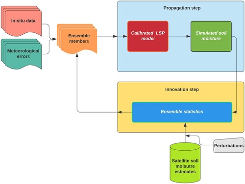
An EnKF-based assimilation framework was implemented to estimate RZSM using the LSP model in Huamantla, Tlaxcala. The methodology of this work is made up of several steps (see Figure 3). First, the database is composed of meteorological information, soil and vegetation parameters obtained from the THEXMEX-18 campaign, and satellite information. Afterwards, a calibration process of the LSP model was performed to obtain the optimal in situ parameters. The next step was the coupling of the LSP model and the EnKF algorithm to conform the assimilation algorithm in order to compare the SM simulations with in situ measurements and SM retrievals from SMAP L2SMP product.

Figure 3. EnKF-based assimilation framework.

4.1. LSP calibration

The LSP model is forced with seven micrometeorological parameters and requires 13 ground surface parameters and 15 parameters related to vegetation. For this work, the soil profile is defined by two layers with different properties. The first layer is from the soil surface (0 m) to 0.20-m depth and the second layer was considered between 0.2 m and 1.7 m. Based on soil texture, the first layer was identified up to a depth of 20 cm, containing the TDR measurements at 2.5, 5, and 10 cm. The next layer contains the measurements at 20 and 30 cm, the optimal case was identified with the method of Pareto front comparing both strata. The parameters that were not possible to obtain from in situ measurements were calibrated using the Monte Carlo method with ranges shown in Table 3, based on the literature. The parameter calibration was conducted using the mean square error as objective function. Soil parameters were calibrated under bare soil conditions and those describing the canopy throughout the vegetated period.

Table 3. Parameters included in the LSP model. The intervals for canopy parameters were from Goudriaan (1977) and ranges for soil parameters were from Rossi and Nimmo (1994).

	Parameter	Description	Interval
CANOPY	$z_{ob}$	Bare soil roughness length (m)	in situ
	x	Leaf angle distribution parameter	${10}^{-2}-2$
	σ	Leaf reflectance	${10}^{-2}-0.5$
	${ϵ}_c$	Canopy emissivity	0.95−0.995
	${ϵ}_s$	Soil emissivity	0.95−0.995
	$c_d$	Canopy drag coefficient	${10}^{-5}-1$
	$i_w$	Canopy wind intensity factor	${10}^{-3}-{10}^2$
	$l_w$	Leaf width (m)	in situ
	$F_b$	Base assimilation rate (kg CO${}_2$/m${}^2$s)	$-{10}^{-8}--{10}^{-10}$
	${ϵ}_{photo}$	Photosynthetic efficiency (kg CO${}_2$/J)	${10}^{-7}-{10}^{-5}$
	$soi{l}_a$	Slope parameter for $r_s$ (m${}^2$s/kg H${}_2$O)	$0-5\times {10}^3$
	$soi{l}_b$	Intercept parameter for $r_s$ (m${}^2$s/kg H${}_2$O)	$0--6\times {10}^2$
SOIL	λ	Pore-size index	0.1−0.9
(0-0.2 m)	${\psi }_0$	Air entry pressure (m H${}_2$O)	0.05−1.0
	$K_{sat}$	Saturated hydraulic conductivity (m/s)	${10}^{-5}-{10}^{-3}$
	ϕ	Porosity $\left(m^3/m^3\right)$	0.2−0.55
SOIL	λ	Pore-size index	0.1−0.9
(0.2-1.7 m)	${\psi }_0$	Air entry pressure (m H${}_2$O)	0.05−1.0
	$K_{sat}$	Saturated hydraulic conductivity (m/s)	${10}^{-5}-{10}^{-3}$
	ϕ	Porosity $\left(m^3/m^3\right)$	0.2−0.55

Table 4. Sources of uncertainty in forcing variables and soil parameters in the LSP model based on (Dunne and Entekhabi 2006; Monsivais-Huertero et al. 2016).

Parameter	Range	Distribution
Short wave radiation	0.9–1.1	Gaussian multiplicative
Air temperature	$-3-3$	Gaussian additive
Relative humidity	$-1-1$	Gaussian additive
Wind speed	$-0.3-0.3$	Gaussian additive
Precipitation	0–1	Poisson
Porosity (layer 1)	$-0.3-0.22$	Gaussian additive
Pore-size index (layer 1)	$-0.55-0.16$	Gaussian additive
Porosity (layer 2)	$-0.3-0.036$	Gaussian additive
Pore-size index (layer 2)	$-0.55-0.0795$	Gaussian additive

To complement the meteorological conditions, the long-wave radiation was calculated as (Idso and Jackson 1969; Satterlund 1979): (11) $R_l=\sigma T_A^4(1-0.261exp(-7.77x{10}^{-4}(273-T_A{)}^2))$(11) where $R_l$ is the long-wave radiation, σ is the Stefan-Boltzmann constant, and $T_A$ is the air temperature. The rest of the parameters were obtained from the in situ stations.

4.2. Assessment of SMAP L2SMP product

The assessment of the SMAP LS2SMP product over the agricultural region of Huamantla is evaluated by comparing the SMAP SM retrievals and the upscaled SM measurements. The upscaled SM is obtained by using the soil-weighted method as recommended by the SMAP team to evaluate the SMAP SM products (Colliander et al. 2017; Bhuiyan et al. 2018). The upscaled SM is computed by: (12) $\begin{array}{cc}S{M}_{S,t}& ={\displaystyle \sum _{i=1}^M{w}_i\overline{S{M}_{i,t}}}\\ {\sigma }_{S,t}& =\sqrt{{\displaystyle \sum _{i=1}^M{w}_i(\overline{S{M}_{i,t}}-S{M}_{S,t}{)}^2}}\end{array}$(12) where SM${}_{S,t}$ is the temporal upscaled SM, ${\sigma }_{S,t}$ is the temporal standard deviation, $w_i$ indicates the weights based on the soil texture map, $\overline{S{M}_i}$ represents the averaged surface SM of all stations located in the i-th soil-texture class. To develop the soil-weighted scaling approach, each in situ surface SM value is identified based on its corresponding soil texture. Then, soil texture data are intersected to the SMAP pixel, and percent area statistics are derived for each of the soil texture types (Colliander et al. 2017). In this work, we use the soil texture map provided by the National Institute of Statistics and Geography of Mexico (INEGI) (2017). The Huamantla region is composed of fluvisol (7.05%), cambisol (47.61%), and regosol (45.34%) (see Table 1).

The performance of the SM from the SMAP L2SMP product is evaluated by the bias (Bias), the Root Mean Square Difference (RMSD), the unbiased RMSD (ubRMSD), and the Pearson correlation coefficient (r). The Bias, RMSD, ubRMSD, and r are evaluated as (Gruber et al. 2020): (13) $\mathrm{B}\mathrm{i}\mathrm{a}\mathrm{s}=\frac{1}{N}\sum _{i=1}^N({\mathrm{S}\mathrm{M}}_{\mathrm{S}\mathrm{M}\mathrm{A}\mathrm{P},i}-{\mathrm{S}\mathrm{M}}_{\mathrm{u}\mathrm{p}\mathrm{s}\mathrm{c}\mathrm{a}\mathrm{l}\mathrm{e}\mathrm{d},i})$(13)

(14) $\mathrm{R}\mathrm{M}\mathrm{S}\mathrm{D}=\sqrt{\frac{1}{N}\sum _{i=1}^N({\mathrm{S}\mathrm{M}}_{\mathrm{S}\mathrm{M}\mathrm{A}\mathrm{P},i}-{\mathrm{S}\mathrm{M}}_{\mathrm{u}\mathrm{p}\mathrm{s}\mathrm{c}\mathrm{a}\mathrm{l}\mathrm{e}\mathrm{d},i}{)}^2}$(14) (15) $\mathrm{u}\mathrm{b}\mathrm{R}\mathrm{M}\mathrm{S}\mathrm{D}=\sqrt{{\mathrm{R}\mathrm{M}\mathrm{S}\mathrm{D}}^2-{\mathrm{B}\mathrm{i}\mathrm{a}\mathrm{s}}^2}$(15) (16) $r=\frac{1}{N-1}\sum _{i=1}^N\left(\frac{{\mathrm{S}\mathrm{M}}_{\mathrm{S}\mathrm{M}\mathrm{A}\mathrm{P},i}-\overline{{\mathrm{S}\mathrm{M}}_{\mathrm{S}\mathrm{M}\mathrm{A}\mathrm{P},i}}}{{\sigma }_{{\mathrm{S}\mathrm{M}}_{\mathrm{S}\mathrm{M}\mathrm{A}\mathrm{P},i}}}\right)\left(\frac{{\mathrm{S}\mathrm{M}}_{\mathrm{u}\mathrm{p}\mathrm{s}\mathrm{c}\mathrm{a}\mathrm{l}\mathrm{e}\mathrm{d},i}-\overline{{\mathrm{S}\mathrm{M}}_{\mathrm{u}\mathrm{p}\mathrm{s}\mathrm{c}\mathrm{a}\mathrm{l}\mathrm{e}\mathrm{d},i}}}{{\sigma }_{{\mathrm{S}\mathrm{M}}_{\mathrm{u}\mathrm{p}\mathrm{s}\mathrm{c}\mathrm{a}\mathrm{l}\mathrm{e}\mathrm{d},i}}}\right)$(16) where SM${}_{\mathrm{S}\mathrm{M}\mathrm{A}\mathrm{P}}$ is SM from the SMAP L2SMP product, SM${}_{\mathrm{u}\mathrm{p}\mathrm{s}\mathrm{c}\mathrm{a}\mathrm{l}\mathrm{e}\mathrm{d}}$ is the upscaled SM, and N is the number of (SM${}_{\mathrm{S}\mathrm{M}\mathrm{A}\mathrm{P},i}$, SM${}_{\mathrm{u}\mathrm{p}\mathrm{s}\mathrm{c}\mathrm{a}\mathrm{l}\mathrm{e}\mathrm{d},i}$) pairs. These pairs are composed of coincident times between SMAP SM retrievals and upscaled SM. In equation (16(16) $r=\frac{1}{N-1}\sum _{i=1}^N\left(\frac{{\mathrm{S}\mathrm{M}}_{\mathrm{S}\mathrm{M}\mathrm{A}\mathrm{P},i}-\overline{{\mathrm{S}\mathrm{M}}_{\mathrm{S}\mathrm{M}\mathrm{A}\mathrm{P},i}}}{{\sigma }_{{\mathrm{S}\mathrm{M}}_{\mathrm{S}\mathrm{M}\mathrm{A}\mathrm{P},i}}}\right)\left(\frac{{\mathrm{S}\mathrm{M}}_{\mathrm{u}\mathrm{p}\mathrm{s}\mathrm{c}\mathrm{a}\mathrm{l}\mathrm{e}\mathrm{d},i}-\overline{{\mathrm{S}\mathrm{M}}_{\mathrm{u}\mathrm{p}\mathrm{s}\mathrm{c}\mathrm{a}\mathrm{l}\mathrm{e}\mathrm{d},i}}}{{\sigma }_{{\mathrm{S}\mathrm{M}}_{\mathrm{u}\mathrm{p}\mathrm{s}\mathrm{c}\mathrm{a}\mathrm{l}\mathrm{e}\mathrm{d},i}}}\right)$(16) ), the overline indicates the mean, and ${\sigma }_{{\mathrm{S}\mathrm{M}}_{\mathrm{S}\mathrm{M}\mathrm{A}\mathrm{P},i}}$ and ${\sigma }_{{\mathrm{S}\mathrm{M}}_{\mathrm{u}\mathrm{p}\mathrm{s}\mathrm{c}\mathrm{a}\mathrm{l}\mathrm{e}\mathrm{d},i}}$ represent the standard deviation of the SMAP L2SMP product and the upscaled SM measurements, respectively.

4.3. Implementation of the EnKF

For this work, the nonlinear propagator mentioned in equation (7(7) $x_t^{i-}=f(x_{t-1}^{i+},u_{t-1}^i,{\theta }_{t-1}^{+},t-1)+{\omega }_{t-1}^i$(7) ) is the LSP model and the SM values describing the soil profile are obtained from the LSP model. The state vector, x, is conformed by the LSP SM estimates from the 35 nodes, as shown in equation (17(17) $x_i=\left[\begin{array}{c}S{M}_{i1}\\ S{M}_{i2}\\ ⋮\\ S{M}_{ik}\end{array}\right]$(17) ). The meteorological forcings are presented as $u_{t-1}^i$, ${\theta }_{t-1}^{+}$ and are the invariant inputs in the LSP model (see equation (7(7) $x_t^{i-}=f(x_{t-1}^{i+},u_{t-1}^i,{\theta }_{t-1}^{+},t-1)+{\omega }_{t-1}^i$(7) )). The SM observations from the THEXMEX-18 are obtained from measurements at 0–5, 10, 20, and 30 cm. (17) $x_i=\left[\begin{array}{c}S{M}_{i1}\\ S{M}_{i2}\\ ⋮\\ S{M}_{ik}\end{array}\right]$(17) For this equation, i is the number of ensemble and k represents the number of nodes representing the soil profile in the LSP model. One hundred ($\mathrm{N}=100$) ensembles realizations were used for assimilation to achieve reliable estimates (Nagarajan et al. 2011; Monsiváis-Huertero et al. 2010).

The 0–5 cm SM represents near-surface soil moisture (SM${}_{0-5\mathrm{c}\mathrm{m}}$), comparable to SM from the SMAP L2SMP product, and the SM at 0–100 cm represents the RZSM. The 0-5 cm SM and RZSM estimates and observations are calculated by the equation: (18) $S{M}_{0-5\mathrm{c}\mathrm{m}}orRZSM=\sum _{i=1}^{k}S{M}_i\mathrm{\Delta }{z}_i$(18) where k indicates the total number of nodes (blocks) within 0–5 cm or the root-zone, $\mathrm{\Delta }{z}_i$ the thickness of the $i^{th}$ node, and $S{M}_i$ the soil moisture at $i^{th}$ node.

Among all the inputs/forcings to the LSP model, precipitation observations typically have the highest errors compared with other micrometeorological parameters. A Gaussian error with zero mean and standard deviation equal to 12% of the observed precipitation value was introduced during events (Habib, Krajewski, and Kruger 2001). An error with a Poisson distribution and 0.45 mean was introduced in the absence of the events. In this paper, forcing variables vary within a physically reasonable range based on (Dunne and Entekhabi 2006; Monsivais-Huertero et al. 2016), as shown in Table 4.

4.3.1. Synthetic and field observations

The synthetic truth was obtained from one of the realizations from an open-loop simulation of the LSP model. The truth was not included in the ensemble of 100 members during the assimilation. The field observations were obtained from the THEXMEX-18 experiment, described in Section 2.2. A Gaussian error with zero mean and standard deviation of 0.02 ${\mathrm{m}}^3$ ${\mathrm{m}}^{-3}$ was added to SM values for both synthetic and field observations, based on field information. The temporal frequency of assimilation for both the synthetic and field observations is every three days at 6 a.m., local time, corresponding to the descending pass of the SMAP satellite.

Different assimilation scenarios with synthetic and field SM observations were performed. The evaluation of the assimilation algorithm was compared by assimilating SM at four depths (0–5, 10, 20, and 30 cm) and SM at 0–5 cm only. This evaluation was used to understand the improvements in the SM estimates over the complete SM profile from the assimilation scenarios.

5. Results

5.1. LSP calibration

The calibration of the LSP model was carried out for different depths within the study area. The depths considered for the calibration were 0–5, 10, 20, and 30 cm. Table 5 presents the calibrated values for soil and vegetation parameters within the LSP model. Overall, the SM values from the calibrated LSP model show an RSMD $<0.0194\left({\mathrm{m}}^3{\mathrm{m}}^{-3}\right)$ (1.94 %SM) at all depths during the THEXMEX-18, indicating a general good agreement with TDR measurements. The highest RMSD was found at 10-cm depth. When comparing the calibrated values with previous calibrations of the LSP model over corn fields reported in the literature (Casanova and Judge 2008), it is found the major differences with previous values are mainly due to the different cultivars of corn and soil type. Casanova and Judge (2008) calibrated the LSP model for sweet corn over a sandy soil, whereas in Central Mexico, farmers cultivate hybrid and creole corns over a sandy loam soil. This impacts the optimal values of the parameters related to the plant growth, such as σ, ${ϵ}_c$, $c_d$, $i_w$, $l_w$, $F_b$, and ${ϵ}_{photo}$. Table 6 shows RMSD at each depth. It is observed that the behavior of the LSP simulations are close to in situ information with an RMSD ranging between 0.0149 and 0.0195 (m${}^3$ m${}^{-3}$) at all depths.

Table 5. Calibrated parameters describing soil and vegetation in the LSP model.

	Parameter	Calibrated value
CANOPY	$z_{ob}$	0.00898
	x	0.62166
	σ	0.15409
	${ϵ}_c$	0.9506
	${ϵ}_s$	0.9698
	$c_d$	0.9953
	$i_w$	33.2099
	$l_w$	0.07790
	$F_b$	$-9.7\times {10}^{-9}$
	${ϵ}_{photo}$	$1.6\times {10}^{-6}$
	$soi{l}_a$	545.77
	$soi{l}_b$	$-562.77$
SOIL	λ	0.5767
(0–0.2 m)	${\psi }_0$	0.0565
	$K_{sat}$	$5\times {10}^{-4}$
	ϕ	0.5273
SOIL	λ	0.8205
(0.2–1.7 m)	${\psi }_0$	0.4049
	$K_{sat}$	$1.37\times {10}^{-5}$
	ϕ	0.51

Table 6. Root mean square difference (RMSD) between SM estimates from the calibrated LSP model and THEXMEX-18 SM observations at depths of 0–5, 10, 20, and 30 cm for the entire growing season of corn.

Depth (cm)	RMSD ( m${}^3$ m${}^{-3}$)
0–5	0.0194
10	0.0197
20	0.0169
30	0.0149

Figure 4 shows the comparison between the SM estimates at depths of 0–5, 10, 20, and 30 cm from the LSP model and THEXMEX-18 observations. For the period of bare soil (DoY 105-160 ), a good agreement is observed between estimates from the LSP model and THEXMEX-18 observations at depths of 0–5 and 10 cm. However during the vegetated period (DoY 160-280), differences up to 3.61% SM, 2.98% SM, 2.76% SM and 1.58% SM at 0–5 cm, 10 cm, 20 cm and 30 cm, respectively, are observed during periods of frequent rainfalls and the late season when the plant is completely developed and the ears are in development. As reported in previous studies, most of the SVAT models fail in estimating SM during rainfall events, as observed in this case. At depths of 20 and 30 cm, the differences between LSP estimates and SM observations reduce, but there are still differences during the presence of rainfall events. It is also noted that after DoY 260, when the corn plant started senescence, the LSP estimates and SM observations reduced their differences because of the effects of the vegetation in the energy balance also reduce. This evidences that the main sources of error during the vegetated period in the LSP SM estimates after calibration come from the vegetation parameters.

Figure 4. Comparison of the SM estimates from the LSP model using the calibrated values and SM observations during the THEXMEX-18 experiment at 36 km over the agricultural area of Huamantla, Tlaxcala, Mexico.

In Figure 4, two anomalous dry periods are identified. The fist one is from DoY 160 to 180, and the second one, from DoY 200 to 220, for which the SM values for both LSP estimates and SM observations are below the wilting point of 0.15 ${\mathrm{m}}^3{\mathrm{m}}^{-3}$ (Inzunza-Ibarra et al. 2018). From DoY 160 to 180, both LSP simulations and field observations indicated an extremely dry period. At depths of 0–5 and 10 cm, both SM estimates and SM observations are very close. However, at depths of 20 and 30 cm, SM observations show drier conditions than the LSP estimates. In contrast, during second dry period from DoY 200 to 220, the SM observations show wetter conditions than the LSP estimates. As observed in Figure 4, around DoY 160, there are different rainfall events reported by the rain gauges that were not captured by the TDR observations. At DoY 210, the intensities in rainfalls reported by the rain gauges are lower to reproduce the SM values using the calibrated LSP model. This indicates that the differences between the SM estimates and SM observations are mainly due to uncertainties in the meteorological forcings provided to the LSP model and misrepresentation of soil parameters during extreme conditions.

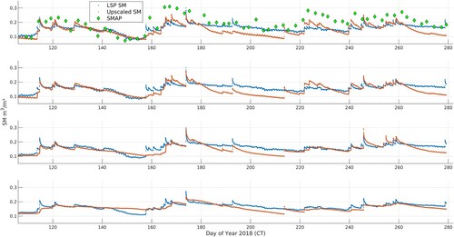
5.2. Performance of the SMAP L2SMP product

The upscaled SM showed a standard deviation $<0.40\left({\mathrm{m}}^3{m}^{-3}\right)$ (40% SM) throughout the THEXMEX-18 when using the soil-weighted method, that is in agreement with previous works (Bhuiyan et al. 2018; Caldwell et al. 2019). The mean value of the coefficient of variation of 0.314 indicates that standard deviation is significantly lower than the mean upscaled SM, assuring representative SM conditions at 36 km. Table 7 presents the statistics of the evaluation for the SCA-V SMAP L2SMP product when compared to the upscaled SM measurements. Overall, the SMAP L2SMP product shows an ubRMSD of 0.043  (m${}^3$ m${}^{-3}$) (4.3% SM) for the agricultural region in Huamantla; thus, the SMAP SM retrievals are close to the SMAP mission requirements of ubRMSD $<0.04\left({\mathrm{m}}^3{\mathrm{m}}^{-3}\right)$ (4% SM) (Entekhabi et al. 2010). It is also observed that the bias is the main component of the difference with in situ SM observations. Because the upscaled in situ SM measurements and the SMAP L2SMP product are at the same spatial scale, the RMSD is primarily due to a composed effect of inaccurate values of the input parameters used in the SMAP SM retrieval algorithm such as surface temperature, vegetation representation, and surface soil roughness (Walker et al. 2019; Judge et al. 2021).

Table 7. Root Mean Square Difference (RMSD), Bias, unbiased RMSD (ubRMSD), and correlation coefficient (r) when comparing the upscaled SM measurements at 0–5 cm with the SM from SMAP L2SMP product and the 0–5 cm SM estimates from the calibrated LSP model at 36-km scale.

	Conditions	RMSD (m${}^3$ m${}^{-3}$)	Bias (m${}^3$ m${}^{-3}$)	ubRMSD (m${}^3$ m${}^{-3}$)	r
SMAP	Overall	0.078	0.065	0.043	0.71
	Bare soil	0.044	0.039	0.022	0.87
	Vegetated	0.085	0.073	0.045	0.61
LSP	Overall	0.032	0.016	0.027	0.72
	Bare Soil	0.020	0.011	0.017	0.92
	Vegetated	0.035	0.017	0.030	0.65

When comparing the statistical metrics for bare soil and vegetated conditions, it is found that the bias and the ubRMSD increment by $0.034({\mathrm{m}}^3{\mathrm{m}}^{-3}$) (3.4% SM) and $0.023\left({\mathrm{m}}^3{\mathrm{m}}^{-3}\right)$ (2.3% SM), respectively, demonstrating that they are time-variant. Variations in the performance of the SMAP L2SMP product have been identified when going from bare soil to vegetated conditions over agricultural regions (Zheng et al. 2020). During bare soil conditions, the bias is the result of uncertainty in effective soil temperature and soil roughness, whereas during vegetated conditions, it is mainly due to uncertainty in vegetation representation (Colliander et al. 2019; Judge et al. 2021). The characterization of the systematic component (bias) and the random component (ubRMSD) of the difference is not an easy task and the SMAP SM retrievals are usually assumed as unbiased when included into an assimilation framework (Mladenova et al. 2019). This is true for regions covered by the SMAP core validation sites; however, it has been demonstrated that this assumption is not valid for other regions (Singh et al. 2019; Zheng et al. 2020). Bias correction methods range from simple algorithms (Ryu et al. 2009) to more complex correction frameworks (Monsivais-Huertero et al. 2016) based on the sources causing the bias. Because the sources of bias in the SMAP SM retrievals do not degrade the mean performance of the retrieval algorithm model according to the SMAP mission requirements of ubRMSD (Colliander et al. 2017), it is possible to use a simple bias-correction method (Ryu et al. 2009). The bias could be considered as constant within specific temporal intervals based on the land cover conditions over the agricultural region. In this study, we correct the bias using a constant value of $0.039\left({\mathrm{m}}^3{\mathrm{m}}^{-3}\right)$ (3.9% SM) for bare soil conditions and $0.073\left({\mathrm{m}}^3{\mathrm{m}}^{-3}\right)$ (7.3% SM) for vegetated conditions based on Table 7.

Table 7 also shows the statistics of the SM estimates at 0–5 cm from the calibrated LSP model when compared to upscaled in situ measurements. It is observed that the ubRMSD from the LSP model and the SMAP L2SMP product is $<0.045\left({\mathrm{m}}^3{\mathrm{m}}^{-3}\right)$ (4.5% SM) for all conditions and both LSP SM estimates and SMAP SM show the same order of magnitude in ubRMSD. Nevertheless, a significant difference is observed when comparing the biases from the LSP SM estimates and the SMAP SM. Whereas the bias from the LSP SM is $<0.017\left({\mathrm{m}}^3{\mathrm{m}}^{-3}\right)$ (1.7% SM), it is $>0.039\left({\mathrm{m}}^3{\mathrm{m}}^{-3}\right)$ (3.9% SM) for the SMAP SM. This indicates that once the bias is corrected, the values from SMAP L2SMP product are comparable to the LSP SM estimates and capture the SM dynamic over the studied region with values close to the actual SM.

5.3. Assimilation of different SM depths

Table 8 presents the RSMD and average standard deviations (ASD) in RZSM when assimilating depths of 0–5, 10, 20, and 30 cm and 0–5 cm only using synthetic and THEXMEX-18 observations. In all cases, the ASD in RZSM reduces by 1.39–1.57 %SM (50–57 %) compared to open-loop when assimilating either 4 depths or 0–5 cm only. This indicates that the assimilation process reduces significantly the uncertainty in RZSM estimates. The highest reduction in the ASD is when assimilating 4 depths.

Table 8. Root mean square differences (RMSD) and average standard deviation (ASD) in RZSM estimates when assimilating synthetic and field observations at depths of 0-5, 10, 20, and 30 cm (4 depths), 0–5 cm only, and SMAP SM retrievals. ubSMAP SM stands for unbiased (bias-corrected) SMAP SM retrievals.

Observations	Depth	Assimilated		Open loop
		RMSD	ASD	RMSD	ASD
		(m${}^3$ m${}^{-3}$)	(m${}^3$ m${}^{-3}$)	(m${}^3$ m${}^{-3}$)	(m${}^3$ m${}^{-3}$)
Synthetic	0–5 cm	0.0155	0.0132	0.0339	0.0276
	4 depths	0.0138	0.0127	0.0339	0.0276
THEXMEX-18	0–5 cm	0.0211	0.0137	0.0243	0.0276
	4 depths	0.0174	0.0119	0.0243	0.0276
ubSMAP SM	0–5 cm	0.0325	0.0142	0.0243	0.0276

For the synthetic case, the assimilation of the 4 depths improves the RZSM estimates by 2 %SM (59%) compared to open-loop, whereas the assimilation of the top 5 cm of the soil improves by 1.8 %SM (54 %). In contrast, the assimilation of 4 depths and 0–5 cm from the THEXMEX-18 experiment improves the RZSM by 0.7 %SM (28%) and 0.3 %SM (13%), respectively, compared to open-loop simulations. As expected, the assimilation of synthetic observations show higher improvement compared to field observations. Synthetic observations were obtained from a LSP simulation; thus, these observations follow the same physics in soil and vegetation presented in the LSP equations (see section 3.1). Unlike synthetic observations, THEXMEX-18 SM observations captured the actual SM conditions in the soil, including heterogeneity in texture between sites and physical processes that could be misrepresented in the LSP model. Beside these sources of error, the percentage of the improvement in RZSM when assimilating real observations over the agricultural area in Central Mexico is about the same order of magnitude than previous studies (e.g Monsiváis-Huertero et al. 2010; Nagarajan et al. 2011).

When comparing the assimilation of 4 depths to the assimilation of 0–5 cm only, it is observed that the improvement in RZSM is about 1.9 %SM (55%) in both cases, compared to open-loop. However, this is also an effect that the synthetic observations follow the same physics than the LSP model. For THEXMEX-18 observations, the assimilation of 0–5 cm only decreases by 3.7%SM (15%) in improving RZSM estimates compared to the assimilation of 4 depths. When assimilating the SM at top 5 cm of the soil, the Kalman equation (see Equation (10(10) $A^{+}=A^{-}+A^{\prime }{A}^{\prime T}{H}^T(H{A}^{\prime }{A}^{\prime T}{H}^T+\gamma {\gamma }^T{)}^{-1}(D-H{A}^{-})$(10) )) propagates statistically the improvement in the top layer into the deeper layers, based on the LSP simulations at the time of the assimilation. Thus, improvement at deeper layers could be affected under certain conditions such as a misrepresentation in the soil strata.

Table 9 compares the SM values at depths of 0–5, 10, 20, and 30 cm after assimilating observations at 4 depths and 0–5 cm only, for both synthetic and THEXMEX-18 observations. For synthetic observations, the improvement in RMSD at all depths is 1.77–2.12 %SM (54–60%) and 1.59–1.96 %SM (48–56%) when assimilating 4 depths and 0–5 cm, respectively, compared to open-loop. In both scenarios of assimilation, the highest improvement occurs at 0-5cm depth, whereas the lowest improvement happens at 30 cm depth. When analyzing the reduction in ASD compared to open-loop, it is found that the enhancement ranges between 1.36–1.54 %SM (52–58%) at all depths when assimilating either 4 depths or 0–5 cm. For THEXMEX observations, the ASD at all depths improves by 1.37–1.6 %SM (52–57%) when assimilating either 4 depths or 0–5 cm only. This indicates that the SM estimates at depths of 0–5, 10, 20, and 30 cm from an assimilation framework increase their certainty when compared to open-loop simulations. In terms of the RMSD, when assimilating 4 depths, it reduces by 1.15%SM (35%) at depths of 0–5 and 10 cm, and by 0.7%SM (25%) at 20 cm. When assimilating 0–5 cm only, the depths of 0–5 and 10 cm improves their SM estimates by 1.2–1.3%SM (36–37%) compared to open-loop, where the SM at 20 cm improves by 0.3%SM (12 %) compared to open-loop. The SM at a depth of 30 cm does not improve when assimilating either the 4 depths or 0–5 cm only. This evidences the fact that the physics of the soil at this depth is not properly represented in the LSP model, despite the calibration process. In order to propagate the improvement in SM estimates at the top 20 cm of the soil, it is necessary to use other assimilation techniques such as the simultaneous state-parameter update (e.g. Monsiváis-Huertero et al. 2010) and obtain a new value in some of the LSP parameters for each assimilation time.

Table 9. Root mean square differences (RMSD) and average standard deviations (ASD) of SM at different depths of the soil when assimilating SM observations at depths of 0–5, 10, 20, 30 cm and 0–5 cm only for synthetic and field observations and unbiased (bias-corrected) SMAP SM retrievals.

		4 depths		0–5 cm		Open loop
Observations	Depth	RMSD	ASD	RMSD	ASD	RMSD	ASD
		(m${}^3$ m${}^{-3}$)	(m${}^3$ m${}^{-3}$)	(m${}^3$ m${}^{-3}$)	(m${}^3$ m${}^{-3}$)	(m${}^3$ m${}^{-3}$)	(m${}^3$ m${}^{-3}$)
Synthetic	0–5 cm	0.0139	0.0114	0.0155	0.0115	0.0351	0.0242
	10 cm	0.014	0.0129	0.0158	0.0133	0.0351	0.0282
	20 cm	0.0151	0.0131	0.0168	0.0136	0.0355	0.0281
	30 cm	0.0152	0.0109	0.017	0.0127	0.0329	0.0263
THEXMEX-18	0–5 cm	0.0238	0.0108	0.0223	0.0123	0.035	0.0242
	10 cm	0.02	0.0122	0.02	0.014	0.0316	0.0282
	20 cm	0.0198	0.0125	0.0232	0.0144	0.0263	0.0281
	30 cm	0.0213	0.0109	0.027	0.0126	0.0208	0.0263
unbSMAP L2SMP	0–5 cm	−	−	0.0334	0.0128	0.035	0.0242
	10 cm	−	−	0.0315	0.0146	0.0316	0.0282
	20 cm	−	−	0.0348	0.015	0.0263	0.0281
	30 cm	−	−	0.0363	0.0131	0.0208	0.0263

Figure 5(a,b) shows the comparison between the time series of the SM at the 0–5 cm and RZSM from open-loop simulations and when assimilating 0–5 cm observations for THEXMEX-18 measurements. This figure depicts that after every point of assimilation, the ensemble standard deviation reduces, and this enhancement is gradually lost as the time goes on. It also is observed that during bare soil conditions (DoY 105–160), both open-loop simulations and SM estimations at 0–5 cm and in the RZSM follow a similar trend than THEXMEX-18 observations even during extreme dry conditions (see for instance DoY 140 to 160). However, when the assimilated values occur close to a rainfall event, the estimations of SM at 0–5 cm and RZSM predict wetter conditions than those described by the in situ observations. This indicates that the drydown in the soil occurs faster than that represented in the LSP equations. This behavior is more evident in the RZSM because the effect of the misrepresentation in the soil infiltration is propagated in all layers. For vegetated conditions (DoY 160–280), open-loop simulations predict wetter conditions than THEXMEX observations for both SM at 0–5 cm and RZSM, particularly from DoY 180 to 220 and from DoY 260 and 280. After assimilating 0–5 cm depth, the SM estimates are closer to in situ observations. Nevertheless, when the assimilated values is outside the region of one standard deviation (represented with a shaded area in the figure), after the assimilation process, the posterior values of SM marginally improve and the physics represented in the LSP model takes back the trend from the SM simulations at both SM at 0–5 cm and RZSM.

Figure 5. Comparison of THEXMEX-18 in situ observations and estimates of (a) SM at 0–5 cm and (b) RZSM when assimilating 0–5 cm SM observations and unbiased (bias-corrected) SMAP SM retrievals, every 3 days. The shaded area represents the standard deviation in the SM estimates.

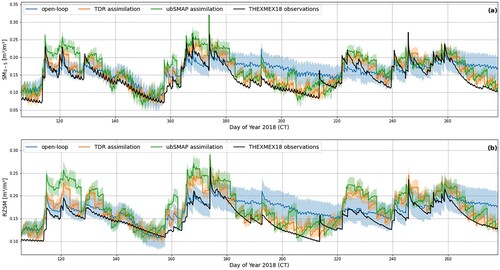
Figure 6(a,b) presents the comparison between the SM estimates at depths of 0–5, 10, 20, and 30 cm from open-loop simulations and when assimilating the THEXMEX-18 observations at 0–5 cm depth. For bare soil conditions, at depths of 10, 20, and 30 cm, both the open-loop simulations and assimilated values of SM follow similar trend as THEXMEX-18 in situ observations, but the assimilated SM estimates obtained closer values to in situ measurements and lower uncertainty than open-loop. For vegetated conditions, field observations are biased low compared to open-loop, primarily under dry periods (DoY 180–220 and 260–280), and although the assimilation algorithm compensates this difference at the 3 depths, the improvement is lost after some points of simulations and SM estimates continue being biased high compared to field observations. As concluded in Monsivais-Huertero et al. (2016), the extended-state-vector technique to update simultaneously states and parameters could be useful to reduce the biases during the assimilation process.

Figure 6. SM estimates at depths of (a) 0–5 cm, (b) 10 cm, (c) 20 cm, and (d) 30 cm from open-loop simulations and when assimilating every 3 days THEXMEX-18 observations at 0–5 cm and unbiased (bias-corrected) SMAP SM retrievals.

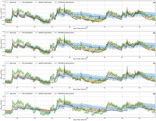
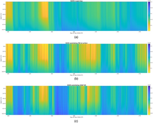
Figure 7 compares the soil moisture profile up to 1-m depth for open-loop simulations and when assimilating 0–5 cm observations during the THEXMEX-18 experiment every 3 days at 6 a.m. It is found that that during bare soil conditions, the LSP model provides SM simulations similar to the assimilation of 0–5 cm from THEXMEX-18 observations up to 1 m. From DoY 140 to 160, both the LSP model and the assimilated SM estimates show dry conditions up to 65 cm, and wetter conditions are observed at deeper layer. During the vegetated period (DoY 160–280), the LSP simulations show wetter conditions for the depths up to 60 cm compared to assimilated in situ observations. At depths deeper than the 60 cm, the LSP simulations and the assimilated SM estimates are closer. This difference could be mainly due to the presence of high root density at the top 60 cm. It is also noted that the effect of a fast infiltration is depicted by the assimilation of THEXMEX-18 observations up to a depth of 70 cm. This indicates that during long dry periods such as DoY 180–220, the plants may suffer of severe water stress if they do not develop roots larger than 65 cm.

Figure 7. Soil moisture profile up to 1-m depth for (a) Open-loop, (b) when assimilating 0–5 cm observations during the THEXMEX-18 experiment every 3 days at 6 a.m., and (c) when assimilating unbiased (bias-corrected) SMAP SM retrievals every 3 days at 6 a.m.

Overall, it was found that the assimilation of 0–5 cm SM observations improved the ASD of the RZSM, comparable to the assimilation of depths at 0–5, 10, 20, and 30 cm. However, the improvement in the RMSD after assimilating of 0–5 cm SM observations reduced when compared to improvement of assimilating four depths. In order to reduce the RMSD in the RZSM, it is necessary to investigate in future works the combination of SM information at depths lower or equal than 30 cm with SM at 0–5 cm.

5.4. Assimilation of SM from the SMAP L2SMP product

Table 8 presents the RMSD and ASD of the RZSM when assimilating unbiased (bias-correct) SMAP SM at 36 km every 3 days. The ASD in RZSM estimates improve by 1.34 %SM (49%) compared to open-loop simulations. However, the RZSM estimates do not improve when assimilating the SMAP SM product, and even worse, the RZSM values are farther way from SM in situ observations. When looking at Table 9, it is observed that only SM estimates at depths of 0–5 and 10 cm marginally improve by 0.1 %SM (4.5%) compared to open-loop simulations. In contrast, SM estimates at depths of 20 and 30 cm are farther way from THEXMEX-18 in situ observations. This lets us conclude that although the certainty in the SM estimates increases, the actual values only marginally improve at the top 10 cm of the soil.

Figure 5 shows the estimates of SM at a depth of 0–5 cm and in the RZSM. When comparing the SM estimates at 0–5 cm and in the RZSM, it is distinguished that the use of SMAP SM retrievals into the assimilation framework improves only the top 5 cm of the soil. This result is in agreement with the values presented in Table 9. This suggests that, to exploit the SMAP SM retrieval and estimates RZSM conditions over agricultural areas in Central Mexico, it is still necessary to improve the satellite SM retrievals. Figure 6 presents the comparison between the SM estimates at depths of 0–5, 10, 20, and 30 cm from open-loop simulations and when assimilating the unbiased SMAP SM retrievals. It is observed that for depths lower than 10 cm, the SM estimates after assimilation do not improve the estimates. The trend in the SMAP SM retrievals produces an erratic trend at depths lower than 10 cm, resulting in SM estimates far away from field observations. In general, the trend from SM estimates are more stable during compared to rainy periods when assimilating SMAP SM retrievals. This behavior explains the statistics presented in Table 9. The information provided by the values from the SMAP SM retrievals is considered by the Kalman equation only when it is within the one-standard-deviation areas, otherwise the assimilation process follows mainly the physics computed in the LSP model. That is why, from DoY 220–240, the posterior SM conditions after assimilation do not represent real SM values according to the LSP equations and the LSP SM simulations go back to open-loop conditions, losing the improvement in the RZSM values.

Figure 7(c) presents the soil moisture profile when assimilating unbiased SMAP SM retrievals every 3 days at 6 a.m. It is found that when using the SMAP information, SM values show wetter conditions for the complete soil moisture profile compared to the assimilation of THEXMEX-18 information. In addition, it is also noted that the SMAP SM retrieval algorithm provide wetter conditions during the presence of rainfalls than field observations. This impacts the SM estimates because after rainfalls with a low intensity, there is a significant increment in the SM values throughout the complete soil moisture profile. The high values of SM from the SMAP retrieval algorithm after rainfalls have been already reported in previous studies such as (Colliander et al. 2017).

Unlike the results presented in Tables 8 and 9 and Figures 5 and 7 (c), studies such as (Mladenova et al. 2019, 2020) have successfully assimilated SMAP information to improve SM estimates at different depths of the soil after correcting the bias. Colliander et al. (2017) showed that most of the core validation sites used to calibrate SMAP SM products show low bias. However, in this study, we monitored an agricultural area that is not included as a core validation site in the SMAP mission. As mentioned in Colliander et al. (2017) and Chan et al. (2016), the accuracy in the SMAP SM retrievals highly depends upon the calibration of the parameter values used in the $\tau -\omega$ model, particularly, on the parametrization to account for roughness and vegetation conditions. Nevertheless, this is not an easy task, for instance, when comparing results from Casanova, Judge, and Jones (2006), Walker et al. (2019) and Judge et al. (2021) over corn fields, it is evidenced that the h-empirical roughness parameter, the b factor, and the vegetation water content have a wider range of values depending upon the corn cultivar. Currently, the soil moisture community needs to exploit measurements from sparse soil moisture networks to characterize regions lacking of information such as Latin America.

In this section, we showed that the assimilation of SM intervals from the SMAP L2SMP product reduced the ASD of the RZSM estimates, compared to open-loop simulation. The RMSD reduced at depths of 0–5 and 10 cm; however, it did not improve when compared to open-loop SM. By using SMAP SM retrievals at 36 km within an assimilation framework, it is possible to infer SM conditions at the top 10 cm, replacing the need of in situ SM sensors. To improve the assimilated SM at depths lower than 20 cm, it is necessary to improve the SMAP SM retrievals and reduce the bias and ubRMSD over agricultural areas before going into an assimilation framework, as reported in Mladenova et al. (2019) and Wigneron et al. (2017). The improvement of SMAP SM retrievals requires collaborative efforts, particularly over regions lacking information. In the next section, we discuss about opened questions remaining about this topic.

6. Discussion

Agricultural regions in developing countries, such as Mexico, affected by a limited infrastructure require information of SM conditions at the root-zone column during regular times with intervals lower than every 2 weeks. More regular information about SM conditions is very useful to understand the effects of the climate change on the precipitation pattern and re-evaluate the plating dates for economic activities based on rainfed local crops, if necessary. This need can be partially covered by passive microwave sensors on-board satellite missions such as the NASA SMAP (Forgotson et al. 2020). Because the penetration of these sensors is limited to the top 5 cm of soil (Ulaby et al. 2014), it is necessary to implement methodologies such as data assimilation to estimate the SM conditions in the root-zone (Reichle et al. 2018). In this work, we found that the standard deviation of RZSM estimates when assimilating in situ SM measurements at 0–5 cm is comparable to that when assimilating SMAP SM retrievals from the L2SMP product with a spatial resolution of 36 km (see Tables 8 and 9). The improvement in the standard deviation indicates that the uncertainty in the value is reduced; thus, the random component of the error is also reduced. However, the RMSD from the RZSM estimates increases when assimilating SMAP SM retrievals by 0.015 (m${}^3$ m${}^{-3}$) when compared to the assimilation of upscaled SM measurements, mainly due to the propagation of systematic errors within the LSP model and the EnKF algorithm. Section 5.4 shows the potential benefit of assimilating bias-corrected SMAP SM retrievals to provide actual conditions in the root-zone column, removing the dependence on in situ SM measurements.

In general, the assimilation frameworks have the drawback that if the observations are more than one standard deviation away from the SM ensemble mean, the updated conditions could produce unrealistic new SM conditions and the improvement from the EnKF will be lost since the physical-based model will be back to the open-loop behavior (Monsiváis-Huertero et al. 2010). For instance, from DoY 220–240, Figure 6 shows that SM observations from the SMAP SM retrievals are more than one standard deviation way from the SM ensemble mean from the LSP model, resulting in loss of the improved conditions and the LSP model brings back the SM conditions into the open-loop estimates. In this case, it is necessary to revise the validity of the assumption of constant parameters within the physical-based model and the reliability of the SM retrievals in that specific period. Studies such as (Monsivais-Huertero et al. 2016) have proposed the implementation of more complex algorithms to correct simultaneously random and deterministic errors into an assimilation framework based on the EnKF. Among different bias correction methods, the simultaneous update of state and parameters within the assimilation framework seems to be the best option due to the computing time and propagation of the updated conditions within the physical-based models. Like the state update only within the EnKF, the main drawback of this technique is that if the observations are more than one standard deviation way from the SM ensemble mean, the updated conditions could produce unrealistic SM conditions and incorrect values in the parameters.

Wigneron et al. (2017) analyze the sources of errors within the SM retrieval algorithms based on passive microwave observations and shows that most of existing assimilation frameworks to improve SM assume bias-corrected observations (e.g. Mladenova et al. 2019). The uncertainty of SM estimates from the SMAP radiometer is a combined effect of calibration of in situ SM sensors (McNairn et al. 2015; Gruber et al. 2020), pixel heterogeneity at the satellite scale (Colliander et al. 2019), the mismatch in the spatial scales between in situ SM measurements and satellite spatial scales observations (Bhuiyan et al. 2018; Caldwell et al. 2019), and the incorrect values in the of the input parameters within the SMAP SM retrieval algorithms (Judge et al. 2021).

In order to minimize the errors due to sensor calibration in this study, we calibrated the SM sensors independently for each field and at each depth using soil samples with a difference $<0.03\left({\mathrm{m}}^3{\mathrm{m}}^{-3}\right)$ when compared to gravimetric SM in all cases (see Section 2.2) similar to previous SM studies (McNairn et al. 2015; Bhuiyan et al. 2018). This methodology was developed during the design of the NASA SMAPVEXs (McNairn et al. 2015) and is suggested to be implemented before evaluating the performance of SM retrievals from satellite observations (Gruber et al. 2020). In these protocols, it is recommended to collect soil samples as frequent as possible during different meteorological conditions to cover a wide range of SM values. However, this condition could impact the representativeness of large regions and the duration of field experiments using temporal and/or sparse SM networks. International collaborative efforts such as the International Soil Moisture Network (Dorigo et al. 2021) and the Joint Experiment for Crop Assessment and Monitoring (JECAM) (Jolivot et al. 2021) have been conforming databases describing soil and vegetation over different biomes worldwide; unfortunately, there are still several regions lacking of information, particularly at tropical latitudes, evidencing the need of additional field experiments contributing in the understanding of these regions.

As shown in Figure 1 and Table 2, the pixel heterogeneity at 36 km was accounted by generating a specific land cover map for the region of Huamantla. Colliander et al. (2019) pointed out the effect of heterogeneity in agricultural regions on SM retrievals when varying the size of the satellite pixels. Efforts such as the collection of the MODIS land cover product (García-Mora, Mas, and Hinkley 2012; Sulla-Menashe et al. 2019) and the ESA Climate Change Initiative's Land Cover (ESA-CCI-LC) dataset (Mousivand and Jokar Arsanjani 2019) can be useful tools since they provide global classification maps; nevertheless, the classifiers implemented still need to be improved by incorporated addition control points over developing countries.

The upscaling method is another aspect that could produce bias in SM retrievals. We generated the upscaled SM using the soil-weighted method as suggested in (Colliander et al. 2017). The standard deviation $<0.40\left({\mathrm{m}}^3{\mathrm{m}}^{-3}\right)$ throughout the THEXMEX-18 and the mean value of the coefficient of variation of 0.314 in the 36-km upscaled SM confirm representativeness of this method over the agricultural region of Huamantla. Bhuiyan et al. (2018) showed that either the soil-weighted method or the Voronoï diagrams can be used to upscale SM at 36 km when using dense SM networks. For sparse networks, Caldwell et al. (2019) shows that it is necessary to verify the standard deviation, the coefficient of variation, and the number of require locations to verify the representativeness of the upscaled SM at each spatial resolution to be evaluated. Because of the lack of representativeness in different sparse SM networks, there is lack of in situ SM information to validate SM products at spatial scales lower than 10 km (Colliander et al. 2017).

Recent studies (Colliander et al. 2019; Judge et al. 2021) have found that the assumption of constant parameters, such as soil roughness and the b factor used to estimate the vegetation optical depth, is not correct since these parameters are time varying and this consideration requires to be re-evaluated to improve the SMAP SM retrievals. Currently, the NASA L2SMP product obtain the values for these parameters based on the lookup table technique based on land cover (O'Neill et al. 2018). In order to obtain the new representation of these parameters, further studies are needed due to diversity and heterogeneity in different biomes worldwide.

7. Conclusions

In this study, an EnKF-based assimilation algorithm was implemented to improve RZSM estimates using the LSP model over an agricultural area of Central Mexico. The objective of this study was to assimilate SM field observations and satellite SM retrievals during a complete growing season of corn to understand the effects of uncertainties in meteorological forcing on RZSM estimates when using the LSP model.

A comparison of EnKF performance using high spatio-temporal density observations from the THEXMEX-18 experiment, synthetic observations, and SM retrievals at 0–5 cm (near-surface SM) from the NASA SMAP mission at 36  km was conducted to differentiate model errors in biophysics from errors in forcings. The SMAP SM retrievals were bias-corrected by identifying the temporal variations of the bias between different land cover conditions. In order to reduce the error in the model representation of the conditions over Central Mexico, the soil and vegetation parameters of the LSP model were calibrated for the complete growing season using the Monte Carlo method. The calibrated values produced an RMSD of 1.69%SM and 1.94%SM in RZSM and near-surface SM, respectively. However, differences between SM estimates from the LSP and SM observations from the THEXMEX-18 remained during frequent rainfall events and during the presence of ears.

Assimilating synthetic observations produced estimates of SM close to the true values throughout the soil profile with an average error of about 1.38% SM (60% reduction of the open-loop RMSE) for the entire growing season. When assimilating THEXMEX-18 observations produced estimates with an average error of about 2.23% SM (36% reduction of the open-loop RMSE) in the top 5 cm. In layers up to 30 cm, the SM had an average error of 1.74% SM (30% reduction of the open-loop RMSE) during the growing season for the THEXMEX-18 observations. This difference between SM errors for the field experiment and synthetic case indicated that simplifications of a homogeneous soil in the LSP model do not represent properly the physics in the soil. When assimilating bias-corrected SM retrievals from the SMAP mission (SMAP L2SMP product), the average error of 3.34% SM (5% reduction of the open-loop RMSE) was observed at the top 0–5 cm with an averaged standard deviation of 1.42% SM. In contrast, the average error in the SM at deeper layers was of 3.25% SM, particularly, over developing countries. The improvement in the soil layers when assimilating SMAP SM retrievals was significantly lower than the assimilation of TDR observations at the top 5 cm of the soil. This indicates that the SM retrievals from satellite missions operating at L-band still need to be improved to infer SM conditions up to 100-cm depth using a data assimilation framework. The improvement in the SM retrievals needs the re-calibration of the main parameters governing the passive signatures from the $\tau -\omega$ model, used as the baseline physical model within the retrieval SM algorithm (Colliander et al. 2017; Chan et al. 2016).

The assimilation of four depths (0–5, 10, 20, and 30 cm) resulted in lower uncertainty in RZSM estimation compared to the assimilation of SM at 0–5 cm only. However, these results demonstrated that SM observations at 0–5 cm, such as those from SMAP mission, could be very useful in an assimilation framework to estimate SM condition up to 10 cm. Although this improvement covers the top 10 cm of the soil, this information could be very valuable particularly on rainfed agricultural regions with lack of information about SM conditions such as Latin America, including Mexico. Frequent information (lower than every 2 weeks) of soil moisture at the top 10 cm of the soil helps to local decision- makers in understanding the local effects of climate change at tropical latitudes.

In this study, only the errors in soil and meteorological forcings were considered. Thus, the observed differences in EnKF performance between synthetic and SM observations may indicate errors in model biophysics that were not considered here, such as constant values in soil parameters or predictions in vegetation description and root distribution. In addition, the SMAP SM retrievals were used in the assimilation algorithm after bias correction based on field experiments. However, it is necessary to use complex bias correction methods in the assimilation algorithms to improve RSZM estimates when exploiting operational satellite SM products for regions without field information available, such as proposed in Moradkhani et al. (2005) and Monsivais-Huertero et al. (2016), or implement methodologies to improve the parameterization in the SMAP SM retrieval algorithm using sparse soil moisture networks covering developing countries.

Acknowledgments

Authors also thank the support from the National Water Commission of Mexico (CONAGUA) to provide the concentrated information about the automatic meteorological stations located in Huamantla, Tlaxcala, during the THEXMEX-18. The authors acknowledge the facilities provided by the farmers from the municipality of Huamantla, Tlaxcala, Mexico.

Data Availability Statement (DAS)

The data that support the findings of this study are available from the corresponding author upon reasonable request.

Disclosure statement

No potential conflict of interest was reported by the author(s).

Additional information

Funding

This work was supported by Consejo Nacional de Ciencia y Tecnología and the Mexican Space Agency [AEM-2017-01-292774], Instituto Politécnico Nacional [SIP-2018-1090, SIP-2020-1876], National Aeronautics and Space Administration [Terrestrial Hydrology Program-NNX16AQ24G].

References

- Altieri, Miguel A, and Javier Trujillo. 1987. “The Agroecology of Corn Production in Tlaxcala, Mexico.” Human Ecology 15 (2): 189–220.
- Bhuiyan, H. A. K. M., H. McNairn, J. Powers, M. Friesen, A. Pacheco, T. J. Jackson, M. H. Cosh, et al. 2018. “Assessing SMAP Soil Moisture Scaling and Retrieval in the Carman (Canada) Study Site.” Vadose Zone Journal 17 (1): 1–14.
- Brandhorst, N, D Erdal, and I Neuweiler. 2017. “Soil Moisture Prediction with the Ensemble Kalman Filter: Handling Uncertainty of Soil Hydraulic Parameters.” Advances in Water Resources 110: 360–370.
- Caldwell, T. G., T. Bongiovanni, M. H. Cosh, T. J. Jackson, A. Colliander, C. J. Abolt, R. Casteel, T. Larson, B. R. Scanlon, and M. H. Young. 2019. “The Texas Soil Observation Network: A Comprehensive Soil Moisture Dataset for Remote Sensing and Land Surface Model Validation.” Vadose Zone Journal 18: 100034.
- Casanova, Joaquin J., and Jasmeet Judge. 2008. “Estimation of Energy and Moisture Fluxes for Dynamic Vegetation Using Coupled SVAT and Crop-Growth Models.” Water Resources Research 44 (7): W07415. doi:10.1029/2007WR006503.
- Casanova, J. J., J. Judge, and J. W. Jones. 2006. “Calibration of the CERES-Maize Model for Linkage with a Microwave Remote Sensing Model.” Transactions of the ASABE 49 (3): 783–792.
- Chan, S. K., R. Bindlish, P. E. O'Neill, E. Njoku, T. Jackson, A. Colliander, F. Chen, et al. 2016. “Assessment of the SMAP Passive Soil Moisture Product.” IEEE Transactions on Geoscience and Remote Sensing 54 (8): 4994–5007.
- Colliander, A., M. H. Cosh, S. Misra, T. J. Jackson, W. T. Crow, J. Powers, H. McNairn, et al. 2019. “Comparison of High-resolution Airborne Soil Moisture Retrievals to SMAP Soil Moisture During the SMAP Validation Experiment 2016 (SMAPVEX16).” Remote Sensing of Environment 227 (15): 137–150.
- Colliander, A., T. J. Jackson, R. Bindlish, S. Chan, N. Das, S. B. Kim, M. H. Cosh, et al. 2017. “Validation of SMAP Surface Soil Moisture Products with Core Validation Sites.” Remote Sensing of Environment 191: 215–231.
- Constantino-Recillas, Daniel Enrique, Eduardo Arizmendi-Vasconcelos, Alejandro Monsivá is-Huertero, José Carlos Jiménez-Escalona, Aura Citlalli Torres-Gómez, Iván Edmundo De La Rosa-Montero, Juan Carlos Hernández-Sánchez, et al. 2020. “Understanding the Backscattering from Sentinel-1 Over a Growing Season of Corn in Central Mexico Using the Thexmex Datasets.” In IGARSS 2020-2020 IEEE International Geoscience and Remote Sensing Symposium, 4526–4529. IEEE.
- De Lannoy, G. J. M., and R. H. Reichle. 2016. “Global Assimilation of Multiangle and Multipolarization SMOS Brightness Temperature Observations Into the GEOS-5 Catchment Land Surface Model for Soil Moisture Estimation.” Journal of Hydrometeorology 17 (2): 669–691.
- Dorigo, Wouter, Irene Himmelbauer, Daniel Aberer, Lukas Schremmer, Ivana Petrakovic, Luca Zappa, Wolfgang Preimesberger, et al. 2021. “The International Soil Moisture Network: Serving Earth System Science for Over a Decade.” Hydrology and Earth System Sciences 25: 5749–5804. doi:10.5194/hess-25-5749-2021.
- Dunne, S. C., and D. Entekhabi. 2006. “Land Surface State and Flux Estimation Using the Ensemble Kalman Smoother During the Southern Great Plains 1997 Field Experiment.” Water Resources Research 41 (1): 04334. doi:10.1029/2005WR004334
- Entekhabi, D., E. G. Njoku, P. E. O'Neill, K. H. Kellogg, W. T. Crow, W. N. Edelstein, J. K. Entin, et al. 2010. “The Soil Moisture Active Passive (SMAP) Mission.” Proceedings of the IEEE 98: 704–716.
- Evensen, Geir. 2003. “The Ensemble Kalman Filter: Theoretical Formulation and Practical Implementation.” Ocean Dynamics 53 (4): 343–367.
- Fernández-Morán, Roberto, J-P Wigneron, Ernesto Lopez-Baeza, Amen Al-Yaari, Amparo Coll-Pajaron, Arnaud Mialon, Maciej Miernecki, et al. 2015. “Roughness and Vegetation Parameterizations At L-band for Soil Moisture Retrievals Over a Vineyard Field.” Remote Sensing of Environment 170: 269–279.
- Forgotson, C., P. E. O'Neill, M. L. Carrera, S. Bélair, N. N. Das, I. E. Mladenova, J. D. Bolten, J. M. Jacobs, E. Cho, and V. M. Escobar. 2020. “How Satellite Soil Moisture Data Can Help to Monitor the Impacts of Climate Change: SMAP Case Studies.” IEEE Journal of Selected Topics in Applied Earth Observations and Remote Sensing 13: 1590–1596.
- Gao, Xiang, Alexander Avramov, Eri Saikawa, and C Adam Schlosser. 2021. “Emulation of Community Land Model Version 5 (CLM5) to Quantify Sensitivity of Soil Moisture to Uncertain Parameters.” Journal of Hydrometeorology 22 (2): 259–278.
- García-Mora, Tziztiki J, Jean-François Mas, and Everett A Hinkley. 2012. “Land Cover Mapping Applications with MODIS: A Literature Review.” International Journal of Digital Earth 5 (1): 63–87.
- Goudriaan, Jan. 1977. “Crop Micrometeorology: A Simulation Study.” PhD diss., Pudoc.
- Gruber, A., G. De Lannoy, C. Albergel, A. Al-Yaari, L. Brocca, J.-C. Calvet, A. Colliander, et al. 2020. “Validation Practices for Satellite Soil Moisture Retrievals: What Are (the) Errors?.” Remote Sensing of Environment 244: 111806.
- Habib, Emad, Witold F Krajewski, and Anton Kruger. 2001. “Sampling Errors of Tipping-bucket Rain Gauge Measurements.” Journal of Hydrologic Engineering 6 (2): 159–166.
- Hanson, J. D., K. W. Rojas, and M. J. Schaffer. 1999. “Calibrating the Root Zone Water Quality Model.” Agronomy Journal 91: 171–177.
- Huang, Chunlin, Xin Li, Ling Lu, and Juan Gu. 2008. “Experiments of One-dimensional Soil Moisture Assimilation System Based on Ensemble Kalman Filter.” Remote Sensing of Environment 112 (3): 888–900.
- Idso, Sherwood B, and Ray D Jackson. 1969. “Thermal Radiation From the Atmosphere.” Journal of Geophysical Research 74 (23): 5397–5403.
- Ines, Amor V. M., Narendra N Das, James W Hansen, and Eni G Njoku. 2013. “Assimilation of Remotely Sensed Soil Moisture and Vegetation with a Crop Simulation Model for Maize Yield Prediction.” Remote Sensing of Environment 138: 149–164.
- Instituto Nacional de Estadística y Geografía (Mé xico). 2017. Guía para la interpretación de cartografía : uso del suelo y vegetación : escala 1:250, 000 : serie VI. Technical Report. Mexico: http://internet.contenidos.inegi.org.mx/contenidos/Productos/prod_serv/contenidos/espanol/bvinegi/productos/nueva_estruc/702825092030.pdf.
- Inzunza-Ibarra, Marco A, María Magdalena Villa-Castorena, Ernesto A Catalán-Valencia, Rutilo López-López, and Ernesto Sifuentes-Ibarra. 2018. “Rendimiento De Grano De Maíz En Deficit Hídrico En El Suelo En Dos Etapas De Crecimiento.” Revista Fitotecnia Mexicana 41 (3): 283–290.
- Jolivot, Audrey, Valentine Lebourgeois, Mael Ameline, Valérie Andriamanga, Beatriz Bellón, Mathieu Castets, and Arthur Crespin-Boucaud, et al. 2021. “Harmonized in Situ JECAM Datasets for Agricultural Land Use Mapping and Monitoring in Tropical Countries.” Earth System Science Data Discussions 1: 1–22.
- Judge, J., P.-W. Liu, A. Monsiváis-Huertero, T. Bongiovanni, S. Chakrabarti, S. C. Steele-Dunne, and D. Preston, et al. 2021. “Impact of Vegetation Water Content Information on SMAP Soil Moisture Retrievals in Agricultural Regions: An Analysis Based on the SMAPVEX16-MicroWEX Dataset.” Remote Sensing of Environment 265: 112623.
- Judge, Jasmeet, Linda M Abriola, and Anthony W England. 2003. “Numerical Validation of the Land Surface Process Component of An LSP/R Model.” Advances in Water Resources 26 (7): 733–746.
- Judge, Jasmeet, Anthony W England, John R Metcalfe, David McNichol, and Barry E Goodison. 2008. “Calibration of an Integrated Land Surface Process and Radiobrightness (LSP/R) Model During Summertime.” Advances in Water Resources 31 (1): 189–202.
- Kerr, Y. H., A. Al-Yaari, N. Rodriguez-Fernandez, M. Parrens, B. Molero, D. Leroux, S. Bircher, et al. 2016. “Overview of SMOS Performance in Terms of Global Soil Moisture Monitoring After Six Years in Operation.” Remote Sensing of Environment 180: 40–63.
- Kolassa, Jana, Rolf H Reichle, Randal D Koster, Qing Liu, Sarith Mahanama, and Fan-Wei Zeng. 2020. “An Observation-driven Approach to Improve Vegetation Phenology in a Global Land Surface Model.” Journal of Advances in Modeling Earth Systems 12 (9): e2020MS002083.
- Kolassa, Jana, Rolf H Reichle, Qing Liu, Michael Cosh, David D Bosch, Todd G Caldwell, Andreas Colliander, et al. 2017. “Data Assimilation to Extract Soil Moisture Information From SMAP Observations.” Remote Sensing 9 (11): 1179.
- Li, Xin, Guodong Cheng, Shaomin Liu, Qing Xiao, Mingguo Ma, Rui Jin, Tao Che, et al. 2013. “Heihe Watershed Allied Telemetry Experimental Research (HiWATER): Scientific Objectives and Experimental Design.” Bulletin of the American Meteorological Society 94 (8): 1145–1160.
- López-Lambraño, Alvaro Alberto, Luisa Martínez-Acosta, Ena Gámez-Balmaceda, Juan Pablo Medrano-Barboza, John Freddy Remolina López, and Alvaro López-Ramos. 2020. “Supply and Demand Analysis of Water Resources. Case Study: Irrigation Water Demand in a Semi-arid Zone in Mexico.” Agriculture 10 (8): 333.
- Maria-Ramírez, A, V. H. Volke-Haller, and M. L. Guevara-Romero. 2017. “Yield Estimation of Native Corn Varieties in the State of Tlaxcala.” Revista Latinoamericana De Recursos Naturales 13 (1): 8–14.
- McNairn, H., T. J. Jackson, G. Wiseman, S. Bélair, A. Berg, P. Bullock, A. Colliander, et al. 2015. “The Soil Moisture Active Passive Validation Experiment 2012 (SMAPVEX12): Prelaunch Calibration and Validation of the SMAP Soil Moisture Algorithms.” IEEE Transactions on Geoscience and Remote Sensing 53 (5): 2784–2801.
- Mladenova, Iliana E, John D Bolten, Wade T Crow, Nazmus Sazib, Michael H Cosh, Compton J Tucker, and Curt Reynolds. 2019. “Evaluating the Operational Application of SMAP for Global Agricultural Drought Monitoring.” IEEE Journal of Selected Topics in Applied Earth Observations and Remote Sensing 12 (9): 3387–3397.
- Mladenova, Iliana E, John D Bolten, Wade Crow, Nazmus Sazib, and Curt Reynolds. 2020. “Agricultural Drought Monitoring Via the Assimilation of SMAP Soil Moisture Retrievals Into a Global Soil Water Balance Model.” Frontiers in Big Data 3: 10.
- Monsiváis-Huertero, Alejandro, Juan Carlos Hernández-Sánchez, José Carlos Jiménez-Escalona, José Mauricio Galeana-Pizaña, Daniel Enrique Constantino-Recillas, Aura Citlalli Torres-Gómez, Ramata Magagi, Kalifa Goïta, and Stéphane Couturier. 2020. “Impact of Temporal Variations in Vegetation Optical Depth and Vegetation Temperature on L-band Passive Soil Moisture Retrievals Over a Tropical Forest Using In-Situ Information.” International Journal of Remote Sensing 41 (6): 2098–2139.
- Monsiváis-Huertero, Alejandro, Juan Carlos Hernández-Sánchez, Iván Edmundo De La Rosa-Montero, Eduardo Arizmendi-Vasconcelos, José Carlos Jiménez-Escalona, Daniel Enrique Constantino-Recillas, Roberto Ivan Villalobos-Martínez, and et al.. 2019. “The Thexmex-18 Dataset: Understanding the Soil and Vegetation Dynamics of Agricultural Fields in Central Mexico from L-Band SMAP Observations.” In IGARSS 2019-2019 IEEE International Geoscience and Remote Sensing Symposium, 6190–6193. IEEE.
- Monsiváis-Huertero, Alejandro, Wendy D Graham, Jasmeet Judge, and Divya Agrawal. 2010. “Effect of Simultaneous State-Parameter Estimation and Forcing Uncertainties on Root-zone Soil Moisture for Dynamic Vegetation Using EnKF.” Advances in Water Resources 33 (4): 468–484.
- Monsivais-Huertero, A., J. Judge, S. Steele-Dunne, and P.-W. Liu. 2016. “Impact of Bias Correction Methods on Estimation of Soil Moisture when Assimilating Active and Passive Microwave Observations.” IEEE Transactions on Geoscience and Remote Sensing 54 (1): 262–278.
- Moradkhani, Hamid, Soroosh Sorooshian, Hoshin V Gupta, and Paul R Houser. 2005. “Dual State-Parameter Estimation of Hydrological Models Using Ensemble Kalman Filter.” Advances in Water Resources 28 (2): 135–147.
- Mountrakis, G., J. Im, and C. Ogole. 2011. “Support Vector Machines in Remote Sensing: A Review.” ISPRS Journal Photogrammetry and Remote Sensing 66 (3): 247–259.
- Mousivand, Alijafar, and Jamal Jokar Arsanjani. 2019. “Insights on the Historical and Emerging Global Land Cover Changes: The Case of ESA-CCI-LC Datasets.” Applied Geography 106: 82–92.
- Nagarajan, Karthik, Jasmeet Judge, Wendy D Graham, and Alejandro Monsivais-Huertero. 2011. “Particle Filter-Based Assimilation Algorithms for Improved Estimation of Root-Zone Soil Moisture Under Dynamic Vegetation Conditions.” Advances in Water Resources 34 (4): 433–447.
- Nair, Akhilesh S, and J Indu. 2019. “Improvement of Land Surface Model Simulations Over India Via Data Assimilation of Satellite-Based Soil Moisture Products.” Journal of Hydrology 573: 406–421.
- O'Neill, P. E., S. Chan, E. J. Njoku, T. Jackson, and R. Bindlish.. 2018. Algorithm Theoretical Basis Document Level 2 and 3 Soil Moisture (Passive) Data Products, Version D. June 6, 2018. JPL D-66480. Technical Report. Pasadena, CA, USA.: Jet Propulsion Laboratory, California Institute of Technology.
- Peischl, Sandy, Jeffrey P Walker, Christoph Rüdiger, Nan Ye, Yann H Kerr, Edward Kim, R Bandara, and Mahdi Allahmoradi. 2012. “The AACES Field Experiments: SMOS Calibration and Validation Across the Murrumbidgee River Catchment.” Hydrology and Earth System Sciences 16 (6): 1697–1708.
- Rautiainen, Kimmo, Juha Lemmetyinen, Jouni Pulliainen, Juho Vehvilainen, Matthias Drusch, Anna Kontu, Juha Kainulainen, and Jaakko Seppanen. 2011. “L-band Radiometer Observations of Soil Processes in Boreal and Subarctic Environments.” IEEE Transactions on Geoscience and Remote Sensing 50 (5): 1483–1497.
- Reichle, Rolf H, Joseph V Ardizzone, Gi-Kong Kim, Robert A Lucchesi, Edmond B Smith, and Barry H Weiss. 2018. Soil Moisture Active Passive (SMAP) Mission Level 4 Surface and Root Zone Soil Moisture (L4_SM) Product Specification Document. Technical Report. Pasadena, CA, USA.: Jet Propulsion Laboratory, California Institute of Technology.
- Reichle, Rolf H, Gabrielle J. M. De Lannoy, Qing Liu, Joseph V Ardizzone, Andreas Colliander, Austin Conaty, Wade Crow, et al. 2017. “Assessment of the SMAP Level-4 Surface and Root-zone Soil Moisture Product Using in Situ Measurements.” Journal of Hydrometeorology 18 (10): 2621–2645.
- Reichle, Rolf H, and Randal D Koster. 2005. “Global Assimilation of Satellite Surface Soil Moisture Retrievals Into the NASA Catchment Land Surface Model.” Geophysical Research Letters 32 (2): 021700.
- Reichle, Rolf H, Randal D Koster, Ping Liu, Sarith P. P. Mahanama, Eni G Njoku, and Manfred Owe. 2007. “Comparison and Assimilation of Global Soil Moisture Retrievals From the Advanced Microwave Scanning Radiometer for the Earth Observing System (AMSR-E) and the Scanning Multichannel Microwave Radiometer (SMMR).” Journal of Geophysical Research: Atmospheres 112 (D9): 08033.
- Rossi, Cinzia, and John R Nimmo. 1994. “Modeling of Soil Water Retention From Saturation to Oven Dryness.” Water Resources Research 30 (3): 701–708.
- Ryu, Dongryeol, Wade T Crow, Xiwu Zhan, and Thomas J Jackson. 2009. “Correcting Unintended Perturbation Biases in Hydrologic Data Assimilation.” Journal of Hydrometeorology 10 (3): 734–750.
- Satterlund, Donald R. 1979. “An Improved Equation for Estimating Long-wave Radiation from the Atmosphere.” Water Resources Research 15 (6): 1649–1650.
- Singh, Gurjeet, Narendra N Das, Rabindra K Panda, Andreas Colliander, Thomas J Jackson, Binayak P Mohanty, Dara Entekhabi, and Simon H Yueh. 2019. “Validation of SMAP Soil Moisture Products Using Ground-based Observations for the Paddy Dominated Tropical Region of India.” IEEE Transactions on Geoscience and Remote Sensing 57 (11): 8479–8491.
- Sulla-Menashe, Damien, Josh M Gray, S Parker Abercrombie, and Mark A Friedl. 2019. “Hierarchical Mapping of Annual Global Land Cover 2001 to Present: The MODIS Collection 6 Land Cover Product.” Remote Sensing of Environment 222: 183–194.
- Torres-Salcido, Gerardo, Rodrigo Meiners-Mandujano, David A Morales-Córdova, Velia Marina-Carral, and Gerardo Alonso-Torres. 2015. “Agricultura Familiar Y Sistema Agroalimentario Localizado: Políticas Locales Para La Producción De Cuitlacoche (Ustílago Maydis Sp.).” Agricultura, Sociedad Y Desarrollo 12 (2): 199–218.
- Ulaby, F. T., D. G. Long, W. J. Blackwell, C. Elachi, A. K. Fung, C. Ruf, K. Sarabandi, H. A. Zebker, and J. van Zyl. 2014. Microwave Radar and Radiometric Remote Sensing. Ann Arbor: University of Michigan Press.
- Velázquez-Cardelas, Gustavo Adrián, Andrés Gonzélez-Huerta, Delfina de Jesús Pérez-López, and Fernando Castillo-González. 2018. “Behavior of Mestizos of Corn in Three Localities of the Center of Mexico.” Revista Mexicana De Ciencias Agrícolas 9 (6): 1217–1230.
- Walker, V. A., B. K. Hornbuckle, Mi.H. Cosh, and J. H. Prueger. 2019. “Seasonal Evaluation of SMAP Soil Moisture in the US Corn Belt.” Remote Sensing 11 (21): 2488.
- Western, A. W., and G. Bloschl. 1999. “On the Spatial Scaling of Soil Moisture.” Journal of Hydrology 217: 203–224.
- Wigneron, J.-P., T. J. Jackson, P. O'Neill, G. De Lannoy, P. De Rosnay, J. P. Walker, P. Ferrazzoli, et al. 2017. “Modelling the Passive Microwave Signatures From Land Surfaces: A Review of Recent Results and Application to the L-band SMOS and SMAP Soil Moisture Retrieval Algorithms.” Remote Sensing of Environment 192: 238–262.
- Wigneron, Jean-Pierre, Mike Schwank, Ernesto Lopez Baeza, Yann Kerr, Nathalie Novello, Cristina Millan, Christophe Moisy, et al. 2012. “First Evaluation of the Simultaneous SMOS and ELBARA-II Observations in the Mediterranean Region.” Remote Sensing of Environment 124: 26–37.
- Yan, Hongxiang, and Hamid Moradkhani. 2016. “Combined Assimilation of Streamflow and Satellite Soil Moisture with the Particle Filter and Geostatistical Modeling.” Advances in Water Resources 94: 364–378.
- Zhao, Tianjie, Jiancheng Shi, Liqing Lv, Hongxin Xu, Deqing Chen, Qian Cui, Thomas J Jackson, et al. 2020. “Soil Moisture Experiment in the Luan River Supporting New Satellite Mission Opportunities.” Remote Sensing of Environment 240: 111680.
- Zhao, Yanxia, Sining Chen, and Shuanghe Shen. 2013. “Assimilating Remote Sensing Information with Crop Model Using Ensemble Kalman Filter for Improving LAI Monitoring and Yield Estimation.” Ecological Modelling 270: 30–42.
- Zheng, Xingming, Zhuang Feng, Hongxin Xu, Yanlong Sun, Yu Bai, Bingze Li, Lei Li, et al. 2020. “Performance of Four Passive Microwave Soil Moisture Products in Maize Cultivation Areas of Northeast China.” IEEE Journal of Selected Topics in Applied Earth Observations and Remote Sensing 13: 2451–2460.