Simultaneous retrieval of land surface temperature and emissivity from the FengYun-4A advanced geosynchronous radiation imager

ABSTRACT

This paper extends a new temperature and emissivity separation (TES) algorithm for retrieving land surface temperature and emissivity (LST and LSE) to the Advanced Geosynchronous Radiation Imager (AGRI) onboard Fengyun-4A, China’s newest geostationary meteorological satellite. The extended TES algorithm was named the AGRI TES algorithm. The AGRI TES algorithm employs a modified water vapor scaling (WVS) method and a recalibrated empirical function over vegetated surfaces. In situ validation and cross-validation are utilized to investigate the accuracy of the retrieved LST and LSE. LST validation using the collected field measurements showed that the mean bias and RMSE of AGRI TES LST are 0.58 and 2.93 K in the daytime and −0.30 K and 2.18 K at nighttime, respectively; the AGRI official LST is systematically underestimated. Compared with the MODIS LST and LSE products (MYD21), the average bias and RMSE of AGRI TES LST are −0.26 K and 1.65 K, respectively. The AGRI TES LSE outperforms the AGRI official LSE in terms of accuracy and spatial integrity. This study demonstrates the good performance of the AGRI TES algorithm for the retrieval of high-quality LST and LSE, and the potential of the AGRI TES algorithm in producing operational LST and LSE products.

KEYWORDS:

• Land surface temperature
• emissivity
• temperature and emissivity separation
• 4SAIL
• water vapor scaling
• geostationary satellite

1. Introduction

As a direct driving factor for land-atmosphere interaction, the land surface temperature (LST) is a critical parameter in climatic, hydrological, ecological, and biogeochemical models (Cheng et al. 2020; Li et al. 2013; Mannstein 1987; Wan and Dozier 1996). Due to its significance in the study of evapotranspiration, climate change, hydrological cycle, drought monitoring, and urban heat island effects (Cheng and Kustas 2019; Kalma, McVicar, and McCabe 2008; Weng 2009; Su 2002; Wan, Wang, and Li 2004; Zhang and Cheng 2019), the LST was identified as one of the essential climate variables (ECVs) (Belward et al. 2016). The land surface emissivity (LSE) is an inherent physical property of the land surface and is primarily regulated by the surface composition and physical state (Cheng et al. 2010; Zhang, Cheng, and Liang 2018; Jiang, Li, and Nerry 2006). The LSE is widely used for target detection and geological mapping based on the characteristics of emissivity spectra (French, Schmugge, and Kustas 2000; Hulley, Veraverbeke, and Hook 2014; Vaughan, Calvin, and Taranik 2003; Kirkland et al. 2002).

In addition to ground measurements and simulation by land surface models, thermal-infrared (TIR) remote sensing is the only means to obtain the LST at regional and global scales. Regarding the TIR satellite remote sensing of LST and LSE, the received top of the atmosphere (TOA) radiance is directly linked to the LST and LSE and coupled with the atmosphere through the radiative transfer equation. Thus, LST and LSE retrieval from TIR TOA radiance is a complex process. Based on the proposed strategies used to solve atmospheric correction and LST and LSE decoupling, scientists have developed a variety of versatile LST retrieval algorithms since the 1980s (Chen et al. 2020; Dash et al. 2002; Zhou and Cheng 2018). According to whether LSE is required to be known a priori, the LST retrieval algorithms can be roughly classified into two types: those with (1) a predetermined LSE in advance, such as the single-channel algorithm (Qin, Karnieli, and Berliner 2001; Jimenez-Munoz and Sobrino 2003; Meng, Cheng, and Liang 2017), the split-window (SW) algorithm (Wan and Dozier 1996; Becker and Li 1990; Yu et al. 2009; Tang et al. 2008), and the multiangle algorithm (Noyes et al. 2007; Ghent et al. 2017); (2) simultaneous retrieval of the LST and LSE, as in the day-night algorithm (Wan and Li 1997), temperature and emissivity separation algorithm (Gillespie et al. 1998), and hyperspectral algorithm (Zhou and Cheng 2018; OuYang et al. 2010; Wang et al. 2011). To determine the LSE, classification-based methods (Snyder et al. 1998; Sobrino et al. 2008; Valor and Caselles 1996) are usually adopted for simplicity and ease of use. LST and LSE simultaneous retrieval algorithms (Zhou and Cheng 2018; Wan and Li 1997; Gillespie et al. 1998; OuYang et al. 2010; Wang et al. 2011; Jiménez-Muñoz et al. 2014) are used to acquire accurate LSE values. With the proposed algorithms mentioned above, many prestigious LST and LSE products have been released to the public, such as the Advanced Spaceborne Thermal Emission and Reflection Radiometer (ASTER) LST and LSE products (Coll et al. 2007; Gillespie et al. 2011), Moderate Resolution Imaging Spectroradiometer (MODIS) LST and LSE products (Wan 2014; Hulley and Hook 2011), Visible Infrared Imaging Radiometer Suite (VIIRS) LST and LSE products (Islam et al. 2017; Wang et al. 2020), Geostationary Operational Environmental Satellites (GOES) LST products (Sun and Pinker 2003) and Spinning Enhanced Visible and Infrared Imager (SEVIRI) LST and LSE products (Peres and DaCamara 2005; Martins et al. 2019; Freitas et al. 2010). Generally, the channel configurations and characteristics of the sensor are the main factors that determine the optimal algorithm.

Recently, with the accumulation of retried LSE products, the composited LSE has been used as an input to the single-channel algorithm and SW algorithm to improve the LSE parameterization. For example, a mean emissivity data set developed by NASA from all available clear-sky ASTER emissivity products between 2000 and 2008, named Advanced Spaceborne Thermal Emission and Reflection Radiometer Global Emissivity Dataset (ASTER-GED) (Hulley et al. 2015), has been used for retrieving LST from VIIRS (Wang et al. 2020), Landsat (Ermida et al. 2020), and Sentinel-3A (Zhang et al. 2019). The Global Land Surface Satellite (GLASS) broadband emissivity product (Cheng and Liang 2014; Cheng et al. 2016) with the 8-day temporal resolution has been used for retrieving LST from China FengYun-3C Medium Resolution Spectral Imager (MERSI) (Meng, Cheng, and Liang 2017). One of the remarkable characteristics of the TES algorithm is that it can obtain LST and LSE at the same time, and the LSE has high accuracy (Hulley, Hook, and Baldridge 2009). If we combine the observations from all the available geostationary satellites, we can obtain hourly global LSE using the TES algorithm and provide near real-time emissivity data for the single-channel and SW algorithms. This is helpful to improve the accuracy of LST retrieval.

FengYun-4A (FY-4A), the second generation of China’s geostationary meteorological satellite, was launched on December 11, 2016 and began operation in 2018 (Chen et al. 2020; Yang et al. 2017). Compared with China’s first-generation geostationary meteorological satellite FengYun-2 (FY-2), FY-4 has improved capabilities for weather and environmental monitoring. FY-4A has four advanced observation instruments – the Advanced Geosynchronous Radiation Imager (AGRI), Geosynchronous Interferometric Infrared Sounder (GIIRS), Lighting Mapping (LMI), and Space Environment Package (SEP). AGRI/FY-4A has four TIR channels and views the disk area (80.6°N-80.6°S, 24.1°E-174.7°W) from longitude 104.7°E. The LST shows strong diurnal variation linked to the surface energy balance and surface thermal inertia, which cannot be easily captured by polar-orbiting satellites. The AGRI can complete at least one disk observation per hour, and has considerable potential for research on diurnal LST variations.

The AGRI/FY-4A provides official LST and LSE products (http://fy4.nsmc.org.cn/portal/en/theme/FY4A.html). The AGRI official LST and LSE are retrieved separately. The AGRI official LST product is produced by the SW algorithm and has not been validated with in-situ measurements (private communication with the principal investigator of the LST product). The AGRI official LSE was retrieved using the physical-based optimization method with an absolute bias larger than 0.01 when compared with the collocated MODIS LSE product (Cao et al. 2018). The spatial resolution of the AGRI official LSE product is 12 km, which is much lower than that of TIR observations. The spatial mismatch between AGRI LST and LSE products may hinder their synergistic use in the surface radiation budget. It is critical to developing an operational algorithm that can be used to simultaneously derive LST and LSE accurately from the AGRI. The AGRI has one TIR spectral channel in the spectral domain of 8–9 μm and two TIR spectral channels in the 10–12 μm atmospheric window and meets the minimum configuration for the development of the temperature and emissivity separation (TES) algorithm (Sobrino and Jimenez-Munoz 2014). The channel configuration of the AGRI provides a precious opportunity to implement the TES algorithm, which is expected to generate accurate spatially matched LST and LSE products.

We have developed a new TES algorithm for the Advanced Himawari Imager (AHI) onboard the geostationary satellite Himawari-8, and achieved an accurate estimate of LST and LSEs from AHI data (Zhou and Cheng 2020). Thus, the objective of the study is to extend the developed TES algorithm for AGRI (named as the AGRI TES algorithm hereafter) to simultaneously derive the LST and LSE from AGRI imagery. This paper is structured as follows. Section 2 provides the details of the AGRI data, auxiliary data, and ground measurements. The theoretical basis of the AGRI TES algorithm is provided in Section 3, and the validation and evaluation results of the retrieved AGRI LST and LSE are presented in Section 4. The discussion and conclusion are presented in Sections 5 and 6, respectively.

2. The data

To develop the AGRI TES algorithm, AGRI L1 full disk data, the corresponding cloud mask product, and geolocation data, along with the Modern-Era Retrospective analysis for Research and Applications version 2 (MERRA-2) data (Gelaro et al. 2017), the SeeBor atmospheric profiles (Borbas et al. 2005), the MODIS vegetation indices product MOD13C1 (Huete et al. 2002), the snow product MOD10C2 (Salomonson and Appel 2004), and the Land Surface Temperature and Emissivity (LST&E) product MOD11C2 (Wan and Li 1997) are needed. Besides, the LST&E product MYD21_L2 (Hulley, Malakar, and Freepartner 2016; Malakar and Hulley 2016), and ground measurements are adopted for the validation. The details of these data are described below.

2.1. FY-4A data

FY-4A data has been released freely to the public since March 12, 2018. AGRI/FY-4A takes 15-min to complete a full-disk scan in 14 spectral channels. The spatial resolutions are 1 km for three visible (VIS) channels, 2 km for four near-infrared (NIR) channels, and 4 km for seven TIR channels at nadir. Table 1 details the characteristics of the AGRI TIR channels, and the corresponding spectral response curves are shown in Figure 1. Only channels 11, 12 and 13 are employed to retrieve the LST and LSE since channel 14 is located in the spectral region with strong atmospheric absorption. In addition, the AGRI multichannel threshold-based cloud mask product is employed to discriminate clear-sky and cloudy sky pixels. One year (April 2018 to March 2019) of AGRI full disk L1 product and cloud mask product were collected to implement the AGRI TES algorithm. The AGRI geolocation data, including (1) the AGRI L1_GEO product, reprocessed after earth navigation from level 0 raw package data, provides the viewing zenith angle of AGRI pixels in the 4 km nominal fixed grid; (2) the AGRI coordinate transformation lookup table that matches the column and line numbers of nominal projection to the geographic latitude and longitude values. These data were downloaded from the data sharing platform of the National Satellite Meteorological Center (http://www.nsmc.org.cn/en/NSMC/Home/Index.html).

Figure 1. Spectral response functions for AGRI TIR channels. The gray dotted line shows the spectral response functions with respect to the functions of MODIS channels 29, 31 and 32.

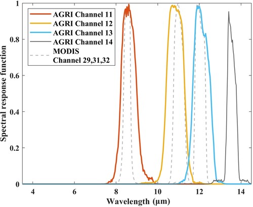
Table 1. Specifications of AGRI TIR channels.

Channel	Central wavelength (μm)	Spatial resolution (km)	Sensitivity (300 K)	Remark
11	8.5	4	NEDT≤0.2K	Atmospheric window
12	10.8	4	NEDT≤0.2K	Atmospheric window
13	12.0	4	NEDT≤0.2K	Atmospheric window
14	13.5	4	NEDT≤0.5K	CO2 absorption

2.2. Auxiliary data

The Modern-Era Retrospective analysis for Research and Applications version 2 (MERRA-2) (Gelaro et al. 2017) analyzed meteorological data inst6_3d_ana_Np provides the needed atmospheric profiles for atmospheric correction. inst6_3d_ana_Np is a 6-hourly pressure-level analyzed meteorological dataset that contains the air temperature, humidity, and geopotential height at 42 pressure levels with a spatial resolution of 0.5°×0.625°. These data are accessible from the Goddard Earth Sciences Data and Information Services Center (https://disc.gsfc.nasa.gov/).

Since AGRI land products only provide the LST and LSE, the required satellite data to develop the TES algorithm primarily come from MODIS. Because the spatial resolution of AGRI TIR data is 4 km at the subsatellite point, MODIS global 0.05°×0.05° climate modeling grid products (MOD13C1, MOD10C2 and MOD11C2) are used in this study. MOD13C1 provides the average 16-day Normalized Difference Vegetation Index (NDVI) calculated and projected using the two 8-day composite surface reflectance granules (MOD09A1) in the 16-day period. The MOD10C2 reports the average 8-day maximum percentage of snow-covered land based on the normalized difference snow index (NDSI). The day/night algorithm-retrieved MODIS LST&E product (MOD11C2) provides average 8-day LSE values. The MODIS data are downloaded from the NASA Earthdata Search (https://search.earthdata.nasa.gov/search). The MOD13C1 NDVI reconstructed by the Savitzky–Golay filter (Chen et al. 2004), the MOD10C2 snow cover and the MOD11C2 LSE are used in the Water Vapor Scaling (WVS) method.

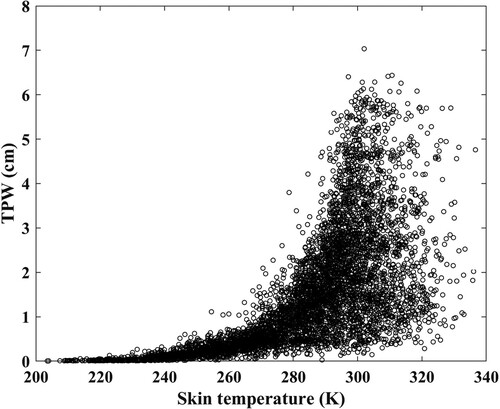
The SeeBor V5.0 atmospheric profile database is used to generate training data for coefficient fitting in the TES. The SeeBor V5.0 database contains 15704 atmospheric profiles of the uniformly distributed global atmospheric sounding temperature, moisture, and ozone at 101 pressure levels. The relative humidity (RH) of the profile is used to exclude the cloudy-sky profile. If the relative humidity (RH) of each layer is greater than 90% or the RH is greater than 85% within two consecutive layers, the profile is labeled a cloudy profile (Cheng, Liang, and Shi 2020). In total, 5578 profiles over the land surface were retained after filtering, and the distribution of total precipitable water vapor (TPW) with skin temperature for these profiles is shown in Figure 2.

Figure 2. Scatterplot of the TPW versus the skin temperature for the selected atmospheric profiles.

2.3. MYD21 product

The MYD21 LST&E product released with MODIS Collection 6, generated by the TES algorithm with the WVS atmospheric correction method, has shown LST accuracies at the ∼1 K level for most cases, compared with the in situ measurements (Malakar and Hulley 2016; Coll et al. 2016). The LSE of MxD21 is in better agreement with the lab values than the classification-based LSE of MxD11, especially for the LSE of band 31 over arid and semiarid areas (Hulley, Malakar, and Freepartner 2016). The MYD21 was adopted for LST&E cross-validation in this article accordingly.

2.4. Ground measurements

The ground-measured surface longwave upwelling radiation (SLUR) and surface longwave downward radiation (SLDR) from 12 flux measurement sites were employed to validate the retrieved LST from AGRI data, including 6 sites from the Heihe Watershed Allied Telemetry Experimental Research (HiWATER) network (Li et al. 2013; Liu et al. 2018) and 6 sites from the Australian and New Zealand flux tower network (OzFlux) (Beringer et al. 2016). Table 2 summarizes the details of the validation sites. These sites include bare soil, maize, grassland, forest, and marsh alpine meadow land cover types. The SLUR and SLDR were primarily measured by CNR1 net radiometers and the Kipp & Zonen CNR4 in HiWATER and OzFlux, respectively. During the HiWATER experiments, the measurement difference of all CNR1/CNR4 net radiometers varied from approximately −8 W/m² in the daytime to 3 W/m² at nighttime, when compared to an Eppley Precision Infrared Radiometer (Xu et al. 2013). The uncertainty of the in situ LST derived from the ground-measured SLUR and SLDR was analyzed in (Zhou and Cheng 2020).

Table 2. Details of the selected sites in the HiWater and OzFlux networks.

Network	Site No.	Site ID	Latitude (N)	Longitude (E)	Land cover	Instrument
HiWATER	1	A’rou(AR)	38.047°	100.464°	Savanna and grassland	CNR1 net radiometers
	2	Daman (DM)	38.856°	100.372°	Maize	CNR1 net radiometers
	3	Dashalong (DSL)	38.840°	98.941°	Marsh alpine meadow	CNR1 net radiometers
	4	Huangmo (HM)	42.114°	100.987°	Bare soil	CNR1 net radiometers
	5	Huazhaizi (HZZ)	38.765°	100.319°	Bare soil	CNR1 net radiometers
	6	Sidaoqiao (SDQ)	42.001°	101.137°	Tamarix	CNR1 net radiometers
OzFlux	7	Cow Bay	−16.238°	145.427°	Forest	Hukseflux NR01
	8	Cumberland Plain	−33.615°	150.724°	Woodland	Kipp & Zonen CNR4
	9	Daly Uncleared	−14.159°	131.388°	Savanna	Kipp & Zonen CNR4
	10	Longreach	−23.523°	144.310°	Grassland	Kipp & Zonen CNR4
	11	Sturt Plains	−17.151°	133.350°	Grassland	Kipp & Zonen CNR4
	12	Yanco	−34.988°	146.291°	Bare soil	Kipp & Zonen CRG4

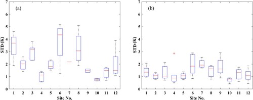
Because the footprint of the ground-based tower measurement is much smaller than the spatial resolution of the AGRI, it must be ensured that measurements at ground sites are representative of the 4 km × 4 km AGRI pixel (Yu et al. 2012; Gottsche et al. 2016). The five-year (2014-2019) ASTER LST product (AST_08) was used to assess the spatial thermal homogeneity of each validation site. The MODIS cloud mask product MOD35_L2 (Ackerman et al. 2010) was used to filter out cloud-contaminated AST_08 images and the retained images were visually inspected. The standard deviations (STDs) of the ASTER LSTs in 45 × 45 ASTER LST 90-m pixels around each site were calculated, and the boxplots of their STDs are shown in Figure 3. LST exhibits much higher spatial homogeneity during the nighttime, with STDs of 45 × 45 ASTER LST subsets less than 2 K in most cases, whereas only approximately half of the sites have relatively acceptable STDs in the daytime. The changing solar radiation leads to rapid spatiotemporal variation in the LST during the day. The LST spatial homogeneity also depends on the satellite overpass time. Note that there are some abnormally high values of the STDs around the Cow Bay site in AST08 due to a forest fire, but no anomalies occurred within the time interval of this study. Accordingly, the outliers of Cow Bay caused by fire were removed in Figure 3.

Figure 3. STD of 45 × 45 ASTER LST subsets around each validation site in (a) daytime and (b) nighttime. In the boxplots, the lines in the middle of the boxes mark the median, and the upper and lower whiskers indicate the maximum and minimum, respectively.

3. Methodology

In the TIR spectral domain, the clear-sky TOA radiance received by the sensor can be divided into three parts: the surface self-emittance, the surface reflected atmospheric downward radiance, and the atmospheric upward radiance. For a certain channel $i$, the TOA radiance is expressed as follows: (1) $L_i\left(\theta \right)=\left({ϵ}_i{B}_i\left(T_S\right)+\left(1-{ϵ}_i\right)L_i^{\downarrow }\right){\tau }_i\left(\theta \right)+L_i^{\uparrow }\left(\theta \right)$(1) where $L_i\left(\theta \right)$ is the TOA radiance; $\theta$ is the viewing zenith angle; ${ϵ}_i$ is the surface emissivity; $T_S$ is the surface temperature; $B_i\left(T_S\right)$ denotes the Planck function at surface temperature $T_S$; ${\tau }_i\left(\theta \right)$ is the transmittance of the total atmosphere; $L_i^{\downarrow }$ is the hemispherical integrated atmospheric downward radiance (abbreviated as atmospheric downward radiance later); and $L_i^{\uparrow }\left(\theta \right)$ is the atmospheric upward radiance (also named the atmospheric path radiance). According to (1), the ground-leaving radiance is expressed as (2) $L_{g,i}\left(\theta \right)={\displaystyle \frac{L_i\left(\theta \right)-L_i^{\uparrow }\left(\theta \right)}{{\tau }_i\left(\theta \right)}={ϵ}_i{B}_i\left(T_S\right)+\left(1-{ϵ}_i\right)L_i^{\downarrow }.}$(2)

Surface temperature and emissivity retrieval from (2) is a tough issue. Assuming that the atmospheric parameters (${\tau }_i$, $L_i^{\downarrow }$ and $L_i^{\uparrow }$) are known or simulated by a radiative transfer model (RTM) with synchronized atmospheric profiles, there are still two unknown variables in (2), namely, the surface temperature and emissivity. Decoupling the surface temperature and emissivity from (2) is an ill-posed problem, i.e. solving one surface temperature and N surface channel emissivities with N channel observations (Li, Strahler, and Friedl 1999). Additional information must be imposed to constrain (2) and make the ill-posed problem well determined. Many strategies have been proposed to separate the surface temperature and emissivity from multichannel TIR observations (Mannstein 1987). Thus, atmospheric correction and temperature and emissivity separation are two essential steps in estimating the surface temperature and emissivity from multichannel TIR observations.

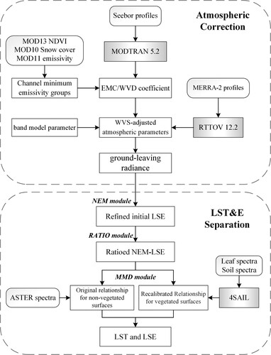
Figure 4 presents the flowchart used to develop the AGRI TES algorithm. There are two key components: atmospheric correction and temperature and emissivity separation. A modified WVS method was conducted for atmospheric correction, which is applicable for both high emissivity (graybody) and low emissivity (nongraybody) pixels. Note the definition of terminology graybody here is different from the standard definition of the gray body in the textbook, so does the definition of nongraybody. For LST and LSE retrieval, a new empirical function is established for vegetated surfaces that explicitly considers the multiple scattering between leaves and the underlying soil background.

Figure 4. Flow diagram summarizing the AGRI TES algorithm.

3.1. Atmospheric correction

Three atmospheric parameters need to be accurately estimated to perform the atmospheric correction. This is realized by feeding the atmospheric profiles into the RTM to simulate the atmospheric parameters. Operationally, a fast RTM such as Radiative Transfer for TOVS (RTTOV) is employed for its higher computational efficiency and relatively acceptable accuracy (Saunders et al. 2018). According to (Matricardi 2009), RTTOV’s simulation agrees with hyperspectral measurements within ±1 K in the atmospheric window. In addition, RTTOV has an obviously faster operation speed than moderate-resolution atmospheric transmission (MODTRAN) (Berk et al. 2005). Thus, RTTOV is employed in the AGRI TES algorithm.

Due to the difficulty of obtaining accurate atmospheric profiles or real-time atmospheric sounding profiles (especially the temperature and water vapor profiles) during the satellite overpass time, reanalysis profiles are typically used as vicarious profiles for TIR atmospheric correction. Compared with accurate radiosonde profiles obtained during the overpass time of the AGRI, MERRA2 atmospheric profiles may have larger errors, which propagate into the simulated atmospheric parameters and ultimately affect the accuracy of the derived LST and LSE. According to previous studies (Gillespie et al. 2011; Li, Becker, et al. 1999; Hulley, Hughes, and Hook 2012; Guillevic et al. 2014), atmospheric profile errors constitute the primary source of errors for the TES algorithm, especially in the case of humid and warm atmospheric conditions. Thus, the WVS method has been proposed (Tonooka 2005, 2001) and used to alleviate the effects of inaccurate atmospheric correction by scaling the reanalysis water vapor profiles on a pixel-by-pixel basis. The WVS method has been incorporated in the operational TES algorithms of MODIS and VIIRS (Islam et al. 2017; Hulley and Hook 2011), and the efficacy of the WVS method in improving the performance of the TES algorithm has been recognized (Li et al. 2019; Tonooka 2000). Therefore, the WVS method is applied in the atmospheric correction for AGRI.

The WVS method was developed from the extended multichannel/water-vapor-dependent (EMC/WVD) algorithm (Francois and Ottle 1996), which originated from an improved SW algorithm for sea surface retrieval (Baldridge et al. 2009). The surface brightness temperatures (BTs) are formulated as quadratic polynomials of TPW and TOA BTs. (3) $L_{g,i}\left(\theta \right)=B_i\left(T_{g,i}\right)={\displaystyle \frac{L_i\left(\theta \right)-L_i^{\uparrow }\left(\theta ,\gamma \right)}{{\tau }_i\left(\theta ,\gamma \right)}}$(3) With $T_{g,i}={\alpha }_{i,0}+\sum _{k=1}^n{\alpha }_{i,k}{T}_k$ ${\alpha }_{i,k}=p_{i,k}+q_{i,k}W+r_{i,k}{W}^2$where $T_{g,i}$ is the surface BT; ${\tau }_i\left(\theta ,\gamma \right)$ and $L_i^{\uparrow }\left(\theta ,\gamma \right)$ are the transmittance and the path radiance corrected by the water vapor profile scaling factor $\gamma$, respectively; $n$ is the number of channels; $T_k$ is the TOA BT measured by channel $k$; $\alpha$, $p$, $q$ and $r$ are the coefficients for each channel; and $W$ is the TPW. Assuming the transmittance of an absorbing molecule is approximated by the Pierluissi double exponential band model (Kneizys et al. 1996): $\tau =\mathrm{e}\mathrm{x}\mathrm{p}\left\{-{\left(CU\right)}^a\right\}$, the total band model transmittance calculated by water vapor profile scaled with $\gamma$ is expressed as (4) $\tau \left(\gamma \right)={\tau }_0\cdot exp\left\{-{\left(C_{\gamma }U\right)}^a\right\}={\tau }_0\cdot ({\tau }_{\omega }{)}^{{\gamma }^a}$(4) where $C$ is the band model absorption coefficient, $U$ is the scaled absorber amount that can be expressed as a function of the air pressure and temperature, $a$ is the band model parameter expressed as a function of the molecule and specific spectral band for that molecule, ${\tau }_{\omega }$ is the water vapor-dependent component of the transmittance for the unscaled profile, and ${\tau }_0$ is the transmittance of other components. Note that the channel index is omitted in (4) for simplicity. Given two different values of ${\gamma }_1$ and ${\gamma }_2$, $\tau \left(\theta ,\gamma \right)$ and $L^{\uparrow }\left(\theta ,\gamma \right)$ for a chosen $\gamma$ value can be expressed as (5) $\tau \left(\theta ,\gamma \right)=\tau (\theta ,{\gamma }_1{)}^{\frac{{\gamma }^a-{\gamma }_2^a}{{\gamma }_1^a-{\gamma }_2^a}}\cdot \tau (\theta ,{\gamma }_2{)}^{\frac{{\gamma }_1^a-{\gamma }^a}{{\gamma }_1^a-{\gamma }_2^a}}$(5) (6) $L^{\uparrow }\left(\theta ,\gamma \right)=L^{\uparrow }\left(\theta ,{\gamma }_1\right)\cdot {\displaystyle \frac{1-\tau \left(\theta ,\gamma \right)}{1-\tau \left(\theta ,{\gamma }_1\right)}.}$(6)

Inserting (5) and (6) into (3) yields the formulation for the scaling factor $\gamma$ (7) $\gamma ={\left({\displaystyle \frac{\ln {\left({\displaystyle \frac{\tau {\left(\theta ,{\gamma }_2\right)}^{{\gamma }_1^a}}{\tau {\left(\theta ,{\gamma }_1\right)}^{{\gamma }_2^a}}\cdot {\displaystyle \frac{B\left(T_g\right)\text{–}{\displaystyle \frac{L^{\uparrow }\left(\theta ,{\gamma }_1\right)}{1-\tau \left(\theta ,{\gamma }_1\right)}}}{L\left(\theta \right)\text{–}{\displaystyle \frac{L^{\uparrow }\left(\theta ,{\gamma }_1\right)}{1-\tau \left(\theta ,{\gamma }_1\right)}}}}}\right)}^{\left({\gamma }_1^a-{\gamma }_2^a\right)}}{\ln \left({\displaystyle \frac{\tau \left(\theta ,{\gamma }_2\right)}{\tau \left(\theta ,{\gamma }_1\right)}}\right)}}\right)}^{\frac{1}{a}}.$(7)

The implementation of the WVS method for atmospheric correction for AGRI requires two types of variables resolved. One is the EMC/WVD coefficient, and the other is the band model parameter. Additionally, we need to obtain the value of the atmospheric downward radiance in (2), which is the required input of the TES algorithm.

3.1.1. Fitting EMC/WVD coefficients

Since the accuracy of the EMC/WVD algorithm degrades for nongraybody pixels, which are defined as pixels with emissivity is less than a predetermined threshold such as 0.96 at all channels (Tonooka 2000, 2005), the original WVS method is only applied to the graybody pixels, i.e. the LSE at all channels is greater than 0.96, as defined in (Tonooka 2005; Zhou and Cheng 2020). The $\gamma$ values for nongraybody pixels are calculated by horizontal interpolation. Islam et al. (2017) refined the original WVS method and applied it to VIIRS data. Recently. Zhou and Cheng (2020) extended the original WVS method to nongraybody pixels via fitting the EMC/WVD coefficients for a series of subranges of minimum channel emissivity and named it as the modified WVS method. They found that the modified WVS method is better than the original WVS method for arid and semiarid areas without nearby graybody pixels, especially in scenarios with a high water vapor content. Therefore, the modified WVS method was employed in this study.

To obtain the EMC/WVD coefficients of the modified WVS method, representative emissivity spectra consisting of 157 samples were selected from the ASTER spectral library (Baldridge et al. 2009) and MODIS UCSB spectral library (http://g.icess.ucsb.edu/modis/EMIS/html/em.html), which contains typical emissivity spectra such as the emissivity spectra of water, snow/ice, vegetation, soils, sands, and rock. The dynamic range of emissivity is between 0.65 and 1. The selected emissivity spectra were convolved with AGRI’s spectral response function for each channel and then divided into six groups based on the minimum channel emissivity: [0.96,1], [0.91,0.96], [0.86,0.91], [0.81,0.86], [0.76,0.81], and [0.71,0.76]. The simulated LSTs are calculated by adding the differences $\delta$T set as −10, −5, 0, 5, 10, and 15 K to the surface air temperature. We set 6 viewing angles between 0-75° at an interval of 15°. In total, 5,254,476 simulations (5578 profiles×157 spectra× 6 $\delta$T) were generated with MODTRAN 5.2 for each viewing angle. With the simulated surface and TOA BT and the TPW of each SeeBor profile, the EMC/WVD coefficients in (3) were derived by using a linear least squares method for each viewing zenith angle and each group of minimum channel emissivities. The fitting results of the EMC/WVD coefficients for graybody pixels are summarized in Table 3.

Table 3. Example of fitted EMC/WVD coefficients for graybody pixels with minimum channel emissivity in [0.96,1]. VA denotes the viewing zenith angle.

VA	$T_{g,i}$	${\alpha }_{i,0}$			${\alpha }_{i,11}$			${\alpha }_{i,12}$			${\alpha }_{i,13}$			RMSE(K)
		$p_{i,0}$	$q_{i,0}$	$r_{i,0}$	$p_{i,11}$	$q_{i,11}$	$r_{i,11}$	$p_{i,12}$	$q_{i,12}$	$r_{i,12}$	$p_{i,13}$	$q_{i,13}$	$r_{i,13}$
0	$T_{g,11}$	−5.386	−7.023	0.816	0.094	0.199	0.046	0.941	0.662	−0.123	−0.011	−0.836	0.075	0.409
	$T_{g,12}$	−1.410	−3.056	−0.151	−0.333	0.196	0.057	1.242	0.748	−0.145	0.098	−0.933	0.089	0.297
	$T_{g,13}$	−1.411	−8.735	1.178	−0.499	0.199	0.069	0.518	1.078	−0.188	0.988	−1.247	0.115	0.471
15	$T_{g,11}$	−5.421	−6.883	0.732	0.082	0.203	0.047	0.969	0.667	−0.127	−0.127	−0.846	0.077	0.414
	$T_{g,12}$	−1.441	−2.983	−0.224	−0.336	0.201	0.059	1.262	0.754	−0.149	0.082	−0.944	0.092	0.304
	$T_{g,13}$	−1.447	−8.653	1.115	−0.500	0.203	0.071	0.550	1.082	−0.192	0.957	−1.255	0.117	0.478
30	$T_{g,11}$	−5.524	−6.389	0.416	0.043	0.218	0.055	1.060	0.686	−0.140	−0.078	−0.881	0.084	0.435
	$T_{g,12}$	−1.541	−2.712	−0.502	−0.346	0.217	0.066	1.227	0.771	−0.163	0.028	−0.979	0.099	0.327
	$T_{g,13}$	−1.570	−8.325	0.863	−0.499	0.216	0.079	0.652	1.091	−0.205	0.854	−1.279	0.125	0.502
45	$T_{g,11}$	−5.651	−5.294	−0.398	−0.030	0.253	0.071	1.236	0.720	−0.169	−0.179	−0.953	0.101	0.481
	$T_{g,12}$	−1.716	−2.048	−1.240	−0.366	0.255	0.081	1.459	0.801	−0.191	−0.084	−1.048	0.116	0.382
	$T_{g,13}$	−1.811	−7.437	0.138	−0.496	0.248	0.092	0.858	1.102	−0.232	0.647	−1.324	0.140	0.552
60	$T_{g,11}$	−5.558	−2.943	−2.772	−0.167	0.341	0.110	1.557	0.786	−0.239	−0.364	−1.116	0.141	0.608
	$T_{g,12}$	−1.841	−0.476	−3.470	−0.415	0.348	0.117	1.721	0.851	−0.258	−0.296	−1.196	0.154	0.533
	$T_{g,13}$	−2.116	−5.155	−2.178	−0.502	0.329	0.129	1.244	1.112	−0.295	0.269	−1.423	0.176	0.681
75	$T_{g,11}$	−2.375	2.342	−15.963	−0.534	0.678	0.298	2.328	0.991	−0.525	−0.780	−1.672	0.290	1.527
	$T_{g,12}$	0.541	3.249	−16.329	−0.643	0.691	0.301	2.413	1.012	−0.535	−0.768	−1.708	0.298	1.506
	$T_{g,13}$	−0.140	0.961	−15.574	−0.499	0.199	0.069	0.518	1.078	−0.188	0.988	−1.247	0.115	1.566

During the atmospheric correction, the minimum channel emissivity is derived from the MOD11C2 LSE product. MODIS channel emissivities were converted to AGRI channel emissivities using the linear functions (8) fitted with the 157 emissivity spectra. The regression coefficients are shown in Table 4. When the group of minimum channel emissivities of each pixel is determined, the EMC/WVD coefficients are obtained with the viewing angle, and then the surface BT $T_{g,i}$ is calculated using (3). $T_{g,i}$ is linearly interpolated when the viewing angle is not equal to the specified values (0°, 15°, 30°, 45°, 60°, or 75°). (8) $E_i^{AGRI}=a_i\cdot E_i^{MODIS}+b_i.$(8)

Table 4. Regression coefficients of (8).

Channel/AGRI	Channel/MODIS	$a_i$	$b_i$	RMSE
11	29	0.9239	0.0706	0.0086
12	31	1.0196	−0.0214	0.0056
13	32	0.9944	0.0045	0.0023

3.1.2. Fitting band model parameter

With the atmospheric transmittance simulated by MODTRAN 5.2 using 5578 selected profiles under different water vapor scaling factors (0.9, 0.7 and 1.0), the band model parameter $a$ in (5) was fitted by the derivative-free optimization method with bound constraints (Larson, Menickelly, and Wild 2019). The regression results are shown in Table 5.

Table 5. Value of band model parameter for AGRI TIR channels in (5).

Channel	$a$	RMSE of $\tau \left(\theta ,\gamma \right)$
11	1.417	4.49E-04
12	1.850	1.17E-04
13	1.775	4.11E-04

3.1.3. Estimating the atmospheric downward radiance

The atmospheric downward radiance is estimated by the following quadratic function of the path radiance at the nadir view (Tonooka, Rokugawa, and Hoshi 1997): (9) $L^{\downarrow }\left(\gamma \right)=a+b{L}^{\uparrow }\left(0,\gamma \right)+c{L}^{\uparrow }(0,\gamma {)}^2$(9) where $L^{\uparrow }\left(0,\gamma \right)$ is the path radiance at the nadir view and $a$, $b$ and $c$ are regression coefficients derived using the least squares method with the simulated $L^{\uparrow }\left(0,\gamma \right)$. In the atmospheric correction, $L^{\uparrow }\left(0,\gamma \right)$ is computed from $L^{\uparrow }\left(\theta ,\gamma \right)$ and $\tau \left(\theta ,\gamma \right)$ at viewing angle $\theta$ (Tonooka, Rokugawa, and Hoshi 1997) (10) $L^{\uparrow }\left(0,\gamma \right)=L^{\uparrow }\left(\theta ,\gamma \right)\cdot {\displaystyle \frac{1-\tau {\left(\theta ,\gamma \right)}^{\cos \theta }}{1-\tau \left(\theta ,\gamma \right)}}$(10)

The values of the regression coefficients of (9) are shown in Table 6.

Table 6. Regression coefficients of (9).

Channel	$a$	$b$	$c$	RMSE of $L^{\downarrow }\left(\gamma \right)$ (W/cm^2/sr/cm^−1)
11	1.315E-9	1.804	−83855.677	7.33E-08
12	5.318E-8	1.718	−60274.528	5.77E-08
13	8.444E-8	1.648	−42554.880	1.07E-07

3.2. Temperature and emissivity separation

The TES algorithm was originally designed to simultaneously retrieve the LST and LSE from the ASTER instrument, the only operational multispectral TIR sensor at that time (Gillespie et al. 1998). TES hybridizes the normalized emissivity method (NEM) module, emissivity ratio module, and maximum-minimum difference (MMD) module. The NEM assumes that the emissivity of a certain channel reaches the initial maximum value and calculates an initial LST for each channel, then iteratively refines the maximum emissivity and updates the initial LST and emissivity values. The NEM emissivities are ratioed to their average value to preserve the spectral shape of the actual emissivities. Finally, the empirical function between the minimum emissivity ${ϵ}_{min}$ and the MMD of the ratioed values is applied to obtain the absolute value of ${ϵ}_{min}$ and recover the amplitude of the LSE spectrum (Matsunaga 1994). Please refer to Gillespie et al. (1998) for the details of the TES algorithm. The accuracy of the ASTER TES algorithm is 0.015 for LSE and 1.5 K for LST (Gillespie et al. 1998). In addition, an independent field validation campaign demonstrated the good performance of the ASTER TES algorithm over sandy areas (Hulley, Hook, and Baldridge 2009).

We fitted the general empirical function for the AGRI in this study. Eighty-nine emissivity spectra, including rocks, soils, water, vegetation (leaf), and ice/snow samples, were selected from the ASTER spectral library and convolved with the AGRI channel response functions to generate the corresponding emissivities for AGRI channels 11-13, which were employed to determine the empirical function (11) ${ϵ}_{min}=-0.731\cdot MM{D}^{0.763}+\mathrm{0.994.}$(11)

The fitted curve is shown in Figure 5 (a). For vegetated surfaces, leaf emissivity spectra from the ASTER and MODIS UCSB spectral libraries are conventionally used to represent canopy emissivity spectra (Gillespie et al. 1998; Berk et al. 2005), leading to an underestimation of the LSE. This can be explained by the cavity effect that results from radiation trapping within the vegetation canopy, especially for intermediate vegetation cover (Jacob et al. 2017). The inappropriate determination of emissivities is one of the primary sources of error in the retrieved LST over vegetated surfaces. Zhou and Cheng (2020) solved this problem by recalibrating a new MMD relationship for vegetated surfaces using the 4SAIL modeled canopy emissivity spectra (Verhoef et al. 2007), in which the cavity effect is explicitly incorporated. We adopted the same method to obtain the canopy emissivity spectra. We selected 15 leaf spectra and 69 soil spectra from the ASTER and MODIS UCSB emissivity libraries and set the spectral interval as 714-1380 cm⁻¹ with a spectral resolution of 1 cm⁻¹. The leaf area index (LAI) was set to 0–7, with intervals ranging from 0.2–0.5. The viewing zenith angle varied from 0° to 75° with an interval of 15°. There are 4 optional leaf inclination distribution functions (LIDFs) in the 4SAIL model. According to Cheng et al. (2016), the accuracy of the emissivity values calculated by 4SAIL using the spherical distribution function was within 0.005 over a fully vegetated surface. The spherical distribution function was selected in this study accordingly. Finally, the spectral angle mapper (SAM) algorithm (Yuhas, Goetz, and Boardman 1992) was adopted to reduce the redundancies of the 4SAIL-modeled emissivity spectra. We obtained 272 emissivity spectra for vegetated surfaces. These spectra were convolved with the AGRI band response functions to generate the corresponding channel emissivity for AGRI channels 11–13 to fit the new function between the ${ϵ}_{min}$ and MMD over vegetated surfaces; the fitted empirical function is shown in Figure 5 (b). (12) ${ϵ}_{min,veg}=-0.880\cdot MM{D}^{0.971}+\mathrm{0.979.}$(12)

Figure 5. The fitted empirical functions for the AGRI. (a) general curve fitted with 89 ASTER emissivity spectra, (b) new curve fitted using 272 4SAIL-simulated emissivity spectra over vegetated surfaces.

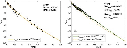
As shown in Figure 5 (b), the general empirical function underestimates ${ϵ}_{min}$ in most cases, whereas the accuracy of the recalibrated new empirical function is fairly good, with an RMSE less than 0.006. The vegetated pixels are identified by the NDVI threshold value of 0.156, as defined in Momeni and Saradjian (2007). When the NDVI is great than 0.156, the pixel is labeled as vegetated and the calibrated function (12) is adopted. The general empirical function (11) is used for bare surfaces, i.e. when the NDVI is less than 0.156.

4. The results

4.1. In situ validation of the LST

Validation is crucial in the development and use of satellite-derived LST and LSE products, which provide the quantitative uncertainty information required for proper applications (Wan 2014; Yu et al. 2012; Ma et al. 2021). In this study, field measurements from the HiWATER network and the OzFlux network were used to evaluate the retrieved LST.

For the selected sites in the HiWATER and OzFlux networks, in situ LST was calculated by the measured surface longwave upwelling and downward radiation using Stefan-Boltzmann's law: (13) $T_S={\left({\displaystyle \frac{L^{\uparrow }-\left(1-{ϵ}_b\right)L^{\downarrow }}{{ϵ}_b\sigma }}\right)}^{\frac{1}{4}}$(13) where $T_S$ is the ground LST; $\sigma$ is Stefan-Boltzmann’s constant (5.67 × 10⁻⁸W/m²/K⁴) and ${ϵ}_b$ is the broadband emissivity obtained from MOD11B1 using the following expression (Cheng et al. 2013). (14) ${ϵ}_b=0.095+0.329\cdot {ϵ}_{29}+0.572\cdot {ϵ}_{31}$(14)

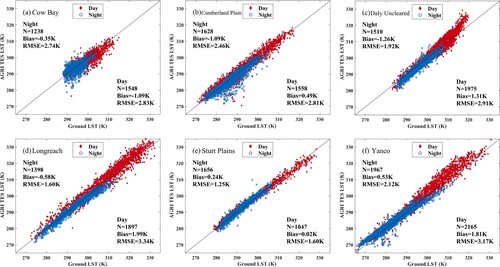
The scatterplots of the retrieved LSTs (AGRI TES LST) versus the in situ LSTs are shown in Figures 6 and 7. The statistical results for each site are shown in Table 2. For the six sites in the HiWATER network, the biases vary from −0.69 K to 0.57 K at nighttime, with an average value of −0.18 K, and from −0.65 K to 1.27 K in the daytime, with an average value of 0.40 K. The RMSE of the LST varies from 1.70 K to 2.92 K at nighttime, with an average value of 2.35 K, and from 2.37 K to 3.60 K in the daytime, with an average value of 3.08 K. For the OzFlux network, the biases vary from −1.09 K to 0.53 K at nighttime, with an average value of −0.42 K, and from −1.09 K to 1.99 K in the daytime, with an average value of 0.76 K. The RMSE of the LST varies from 1.25 K to 2.74 K at nighttime, with an average value of 2.02 K, and from 1.60 K to 3.34 K in the daytime, with an average value of 2.78 K. For the sites of both networks, the LST is in better agreement with the in situ LST during nighttime than in daytime due to its relatively lower heterogeneity. The overall bias and RMSE against the ground measurements are 0.58 and 2.93 K in daytime and −0.30 K and 2.18 K at nighttime, respectively.

Figure 6. Validation results of the AGRI TES LST for HiWATER observations. (a) AR, (b) DM, (c) DSL, (d) HM, (e) HZZ, and (f) SDQ.

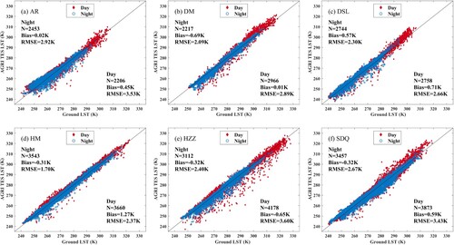
Figure 7. Validation results of the AGRI TES LST for OzFlux observations. (a) Cow Bay, (b) Cumberland Plain, (c) Daly Uncleared, (d) Longreach, (e) Sturt Plains, and (f) Yanco.

The AGRI official LST product was also evaluated by the same in situ measurements at the above stations. The NSMC has provided official LST products since August 2019, and we downloaded one year (August 2019 to July 2020) of AGRI official LST data from NSMC. Note that the HiWATER network covers only the last five months of 2019 for now and two site observations (DSL and HZZ) were not completely updated during this period, the remaining ten sites were adopted to validate the AGRI official LST product accordingly. A systematic underestimation of the AGRI official LST is revealed in Table 7. The scatterplots of the AGRI official LSTs versus the in situ LSTs are provided as supplementary materials for simplicity. Regarding the four sites in the HiWATER network, the biases and RMSEs of the AGRI official LST are −1.04 K and 2.69 K at nighttime and −1.07 K and 3.14 K in the daytime, respectively. However, a large bias (−2.25 K at nighttime and −2.69 K in the daytime) was observed in the OzFlux network, and the corresponding RMSEs are 3.72 K and 4.78 K, respectively. Compared with the official LST, the AGRI TES LST is in better agreement with the in situ LST.

Table 7. Validation results of AGRI official LST during night-time (daytime).

Site ID	N	Bias (K)	RMSE (K)
AR	1551 (1159)	−0.92 (−0.82)	3.15 (3.53)
DM	1338 (1671)	−0.24 (−0.50)	2.26 (3.47)
HM	1699 (1599)	−2.06 (−1.73)	3.09 (2.95)
SDQ	1761 (1826)	−0.53 (−0.79)	2.31 (2.68)
Total	6396 (6357)	−1.04 (−1.07)	2.69 (3.14)
Cow Bay	770 (1148)	−3.95 (−3.68)	5.28 (4.87)
Cumberland Plain	1884 (1956)	−3.38 (−2.61)	4.87 (4.63)
Daly Uncleared	1921 (2199)	−2.79 (−2.32)	3.33 (4.68)
Longreach	1381 (1886)	−1.61 (−2.42)	2.67 (4.38)
Sturt Plains	1147 (1459)	−0.02 (−3.00)	2.38 (5.67)
Yanco	1503 (1488)	−1.55 (−2.62)	3.22 (4.61)
Total	8606 (10136)	−2.25 (−2.69)	3.72 (4.78)

4.2. LST diurnal variation

To test the consistency between the derived clear-sky hourly LSTs within a day, a two-part semi-empirical diurnal temperature cycle (DTC) model, developed by Gottsche and Olesen (2001) and then modified by Jiang, Li, and Nerry (2006) (abbreviated as JNG06 model), was used to fit the DTCs for different land cover types. According to Duan et al. (2012), the JNG06 model has one of the best performances among the six models that fit the DTCs using in situ and MSG/SEVIRI derived LSTs covering the entire day, with a RMSE of approximately 0.5 K. The JNG06 model is expressed by: (15) $T_1\left(t\right)=T_0+T_a\cos \left(\text{β}\left(t-t_m\right)\right),t<t_s$(15) (16) $T_2\left(t\right)=b_1+b_{2}exp\left(\alpha \left(t-t_s\right)+\delta T\right),t\ge t_s$(16)

With $b_1=T_0+T_a\sin \left(\text{β}\left(t_s-t_m\right)\right)-b_2$ $b_2=\left[-\text{β}{T}_a\sin \left(\text{β}\left(t_s-t_m\right)\right)\right]/\alpha$where $T_0$ is the residual temperature around sunrise, $T_a$ is the temperature amplitude, $t_m$ is the time when the temperature reaches its maximum, $t_s$ is the starting time of the free attenuation, $\alpha$ is the decay coefficient, and $\text{β}$ is the angular frequency.

The six free parameters in the JNG06 model were fitted by the derived AGRI LSTs. The initial values of the free parameters were the same as those set in Duan et al. (2012). We randomly selected pixels from typical land cove types within relatively large and homogeneous areas and fitted the diurnal cycles of the derived LSTs (Hong et al. 2018). Table 8 shows the details of the selected pixels. The fitting results as well as the collocated LSTs from the MYD21 are shown in Figure 8. There are no large fluctuations between the derived LSTs and their neighbors. The JNG06 fitted LSTs agree well with the derived LSTs with RMSEs ranging from 0.35 K to 0.55 K for different land cover types. The fitting accuracy is consistent with that of Duan et al. (2012). The result shows that the MYD21 LSTs are consistent with the derived AGRI LSTs as well as the fitted DTC curves. As a result, good consistency exists between the derived LSTs over an entire day for different land cover types.

Figure 8. The diurnal temperature variations of different land cover types fitted by the JNG06 model from the derived AGRI LSTs.

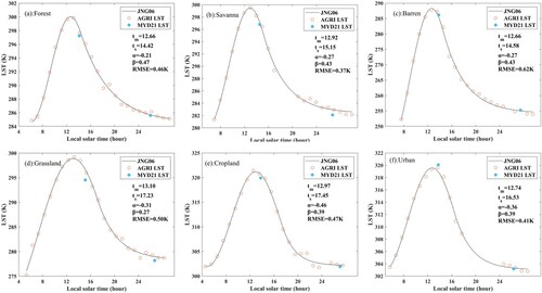
Table 8. Detailed descriptions of the selected pixels used for fitting the DTCs.

Pixel ID	Date	Latitude (N)	Longitude (E)	Land Cover
a	02 Jan 2019	24.264°	95.981°	Forest
b	27 Jan 2019	23.632°	105.556°	Savanna
c	31 Jan 2019	40.037°	99.684°	Barren
d	20 Jul 2018	34.987°	97.455°	Grassland
e	21 Jul 2018	33.454°	116.180°	Cropland
f	29 Jul 2018	24.539°	117.985°	Urban

4.3. LST cross-validation

To further assess the performance of the AGRI TES algorithm as well as the improvement of the AGRI TES algorithm in comparison with the SW algorithm for the AGRI, MYD21 LST, and the AGRI official LST were adopted for intercomparison.

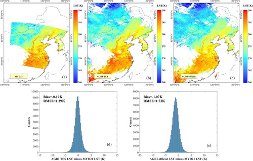
Figure 9 shows the comparison results for the three LSTs in mid-eastern China. The AGRI TES LST and MODIS LSTs are spatially consistent. However, the AGRI official LST is generally lower than the MODIS LST and AGRI TES LST, especially in eastern China. Compared with the MODIS LST, the bias and RMSE of this case are −0.19 K and 1.29 K for the AGRI TES LST, respectively, and −1.07 K and 1.73 K, respectively, for the AGRI official LST.

Figure 9. Comparison between two types of AGRI LSTs (October 30, 2019, 1815 UTC) and the MODIS LST (October 30, 2019, 1815 UTC) in mid-eastern China. (a) MODIS LST. (b) AGRI TES LST. (c) AGRI official LST. (d) histogram of the differences between the AGRI TES LST and MODIS LST. (e) histogram of the differences between the AGRI official LST and MODIS LST.

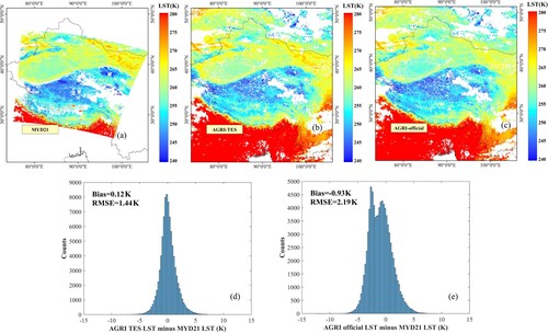
The comparison results for the three LSTs over northwestern China are shown in Figure 10. The spatial distributions of the three LSTs are relatively consistent in this case, except for some underestimated areas around the western part of Inner Mongolia in the AGRI official LST. Compared with MODIS LST, the bias and RMSE are 0.12 K and 1.44 K for the AGRI TES LST, respectively, and −0.93 K and 2.19 K, respectively, for the AGRI official LST.

Figure 10. Comparison between two types of AGRI LSTs (December 8, 2019, 2000 UTC) and the MODIS LST (December 8, 2019, 2000 UTC) over northwest China. (a) MODIS LST. (b) AGRI TES LST. (c) AGRI official LST. (d) histogram of the differences between the AGRI TES LST and MODIS LST. (e) histogram of the differences between the AGRI official LST and MODIS LST.

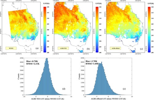
Figure 11 shows the comparison results in east-central Australia. The overpass time of the MODIS LST was 0400 UTC on August 13, 2019. The spatial distributions of the corresponding AGRI TES LST are similar to those of the MODIS LST. However, there are some obvious underestimated areas in the AGRI official LST when compared with the MODIS LST and AGRI TES LST. Taking the MODIS LST as a reference, the bias and RMSE of the AGRI TES LST are −0.70 K and 2.21 K, respectively, whereas the bias and RMSE are −2.70 K and 3.48 K, respectively, for the AGRI official LST.

Figure 11. Comparison between two types of AGRI LSTs (August 13, 2019, 0400 UTC) and the MODIS LST (August 13, 2019, 0405 UTC) in east-central Australia. (a) MODIS LST. (b) AGRI TES LST. (c) AGRI official LST. (d) histogram of the differences between the AGRI TES LST and MODIS LST. (e) histogram of the differences between the AGRI official LST and MODIS LST.

The three case studies show that the spatial distributions of the AGRI TES LST and MODIS LST are highly consistent, and the LST differences are within 5 K under most conditions. However, the AGRI official product obviously underestimates the LST in several areas. The average bias and RMSE of the AGRI TES LST are −0.26 K and 1.65 K, respectively, whereas the average bias and RMSE are −1.57 K and 2.47 K, respectively, for the AGRI official LST.

4.4. LSE cross-validation

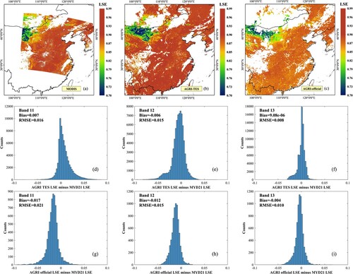
Since the configurations of MODIS channels 29, 31 and 32 are similar to the three AGRI TIR channels used for TES (Figure 1), the MYD21 product was also used to evaluate the derived LSE (AGRI TES LSE) and the AGRI official LSE. A comparison of the MODIS LSE (September 28, 2019, 1815 UTC) and the AGRI TES LSE (September 28, 2019, 1815 UTC) around mid-eastern China is shown in Figure 12. The AGRI TES LSE for channel 11 is similar in spatial distribution to the MODIS LSE for channel 29. The bias and RMSE of the AGRI TES LSE are 0.007 and 0.016, −0.006 and 0.015, 9.08E-06 and 0.008 for channels 11-13, respectively. Compared with the MODIS LSE, underestimates are ubiquitous in the map of the AGRI official LSE. In addition, the coarser resolution causes the AGRI official LSE to lose spatial details, and thus it is not as complete as the AGRI TES LSE. The bias and RMSE of the AGRI official LSE are −0.017 and 0.016, −0.012 and 0.015, −0.004 and 0.010 for channels 11-13, respectively. These results are consistent with Cao et al. (2018). Taking the MODIS LSE as a reference, the AGRI TES LSE outperforms the AGRI official LSE in terms of accuracy (bias) and spatial completeness.

Figure 12. Comparison of two types of AGRI LSEs and MODIS LSE around mid-eastern China. (a) MODIS channel 29 LSE. (b) AGRI TES LSE for channel 11. (c) AGRI official LSE for channel 11. (d-f) histograms of the differences between the AGRI TES LSE and MODIS LSE for channels 11-13. (g-i) histograms of the differences between the AGRI official LSE and MODIS LSE for channels 11-13.

5. Discussion

5.1. Performance of the AGRI TES algorithm for simulation data

MODTRAN 5.2 was used for investigating the effects of the employed modified WVS method as well as the recalibrated MMD function over vegetated surfaces. A total of 240 atmospheric profiles with the TPWs roughly evenly distributed in the range of 0–7 cm were randomly selected from the 5578 SeeBor profiles in Section 2. For each profile, LST was obtained from the ground air temperature with a mean air temperature of +3 K and an STD of 9 K; a total of 272 4SAIL-modeled emissivity spectra were used to fit Equation (12(12) ${ϵ}_{min,veg}=-0.880\cdot MM{D}^{0.971}+\mathrm{0.979.}$(12) ) and five viewing angles (0°, 11.6°, 26.1°, 40.3° and 53.7°) were considered in the simulation. In total, we created 326,400 samples (240 profiles × 1 LST × 272 spectra × 5 angles). The simulated TOA BTs were added random noise with zero mean and 0.2 K standard deviation, which is equal to the NEDT of three AGRI TIR channels. Besides, we perturbed the initial atmospheric profiles followed the strategy of Hulley, Hughes, and Hook (2012): the temperature profile was added a constant 2 K error above the 700 hPa level and a linearly increasing error from 2 K at the 700 hPa pressure level to 4 K at the surface, and the water vapor profile was scaled by the factor generated from random numbers uniformly distributed in the interval [0.8, 1.2].

The simulated data were used to perform the temperature and emissivity separation experiment. The LST and LSE were derived with the original TES algorithm (denoted as TES), its modified WVS version (denoted as TES-WVS), and the TES version with the modified WVS and the new empirical function (denoted as TES-new): the results from these three TES variants were validated against in-situ LST and compared against MODIS MOD21 LST and LSE. After removing the derived LSE without physical meaning, i.e. channel emissivity is less than 0 or greater than 1 (usually caused by the TES algorithm not being able to converge), 306,265 samples were retained. The results are presented in Figures 13 and 14.

Figure 13. The performance of the TES algorithm when tested with simulated data: histogram of the LST differences between the (a) TES LST and true LST; (b) TES-WVS LST and true LST; (c) TES-new LST and true LST.

Figure 14. The performance of the TES algorithm when tested with simulated data: histogram of the LSE differences between the: (a, d, g) TES LSE and true LSE; (b, e, h) TES-WVS LSE and true LSE; (c, f, i) TES-new LSE and true LSE.

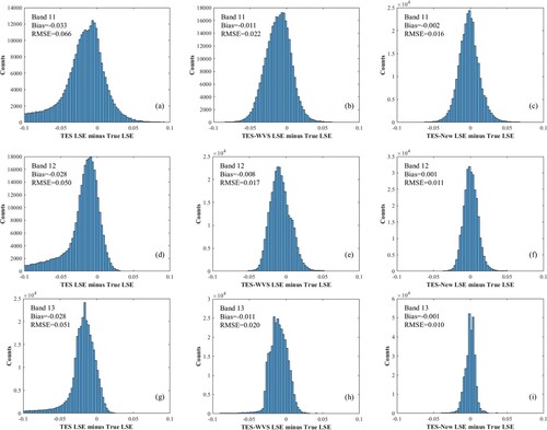
In Figure 13, the TES LST has a bias of 1.31 K and an RMSE of 3.18 K. Clearly, the WVS method improves the LST retrieval accuracy, with a bias of 0.40 K and an RMSE of 1.17 K for the TES-WVS LST, whereas those of the TES-new LST are 0.02 and 0.95 K, respectively. The WVS method remarkably improves the accuracy of LST retrieval for the TES algorithm.

Figure 14 reveals that the TES underestimates LSE in most cases, and the error of channel 11 is the largest, with a bias and an RMSE of −0.033 and 0.066, respectively. When the WVS method is incorporated into the TES algorithm, the error of the derived LSE is dramatically reduced but the LSE is still partly underestimated, with biases of −0.011 for channel 11, −0.008 for channel 12, and −0.011 for channel 13. The AGRI TES-new LSE shows the highest accuracy for all three channels, with absolute biases ≤ 0.002 and RMSEs < 0.02. Comparison of the accuracy of the TES-WVS LSE and TES-new LSE shows that the recalibrated new empirical function eliminates the underestimation of the original empirical function over vegetated surfaces.

In summary, the experimental study demonstrates that the WVS method is a key process of atmospheric correction in the retrieval of LST and LSE using the TES algorithm. The modified WVS method significantly reduces the underestimation of LSE as well as the overestimation of the LST. When the recalibrated empirical function is applied to the TES algorithm, the accuracy of the LST and LSE is further improved. By incorporating the modified WVS method and the recalibrated empirical function, the AGRI TES algorithm effectively removes the deviation of the TES-derived LST and LSE over vegetated surfaces.

5.2. Added value of the derived LSE

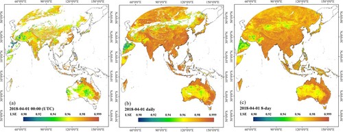
The AGRI TES algorithm generates the hourly LSE data for the full disk. Thus, we can obtain up to 24 emissivity values for each pixel per day. Assuming surface emissivity does not change, we can improve the spatial coverage of emissivity by maximum value or mean value compositions from the retrieved emissivities. Taking one of the channels used by the SW algorithm as an example, we showed the full disk LSE of channel 12 at 0:00 UTC, April 1, 2018, as well as the daily maximum emissivity composition and eight-day mean value composited emissivity in Figure 15. The instantaneous LSE at 0:00 UTC is heavily contaminated by cloud and the spatial coverage is only 45.4%, whereas the spatial coverage of daily maximum composite LSE is increased to 87.4%. The spatial coverage of eight-day mean value composited emissivity was as high as 99.5%. It is a reasonable assumption that surface LSE does not change significantly over several days in most situations (Cheng and Liang 2014; Li et al. 2013). Therefore, the daily or eight-day mean value composited LSE can be used as a priori value in the SW algorithm. Compared to the LSE determined by the classification-based method and vegetation cover method, the derived LSE in this study should be helpful in improving the LST retrieval accuracy of Fengyun series satellites. We believe this is the added value of this study. Certainly, it has great potential to obtain the high spatial average of daily or eight-day composited global LSE through the combination of geostationary satellites and facilitate the usage of SW algorithms.

Figure 15. Maps of AGRI TES LSE for channel 12. (a) The retrieved LSE (0:00 UTC April 1, 2018). (b) The daily maximum composition LSE (April 1, 2018). (c) The eight-day mean composition LSE (April 1-8, 2018).

6. Conclusion

We extended a new TES algorithm for AGRI/FY-4A to accurately obtain spatially matched LST and LSE. The extended TES algorithm was named the AGRI TES algorithm and employs a modified WVS method to achieve accurate atmospheric correction based on MERRA-2 reanalysis profiles and the RTTOV RTM. When compared to the original WVS method, the modified WVS method can directly calculate the water vapor scaling factor for all surfaces using the initial minimum emissivity value of the AGRI TIR channels. The AGRI TES algorithm recalibrates the MMD empirical function over vegetated surfaces using the 4SAIL simulated canopy emissivity spectra. The recalibrated empirical function avoids the underestimation of the empirical function fitted using emissivity spectra of leaves only.

One-year (April 2018 to March 2019) LST and LSE data were generated by the AGRI TES algorithm for the purposes of validation and cross-validation. According to the evaluation against ground measurements collected from the HiWATER and OzFlux networks, the bias and RMSE of the AGRI TES LST are 0.58 and 2.93 K in the daytime, respectively, and −0.30 and 2.18 K in the nighttime, respectively. The AGRI official LST product was also validated by the HiWATER and OzFlux networks. The validation results indicate that the AGRI official LST is systematically underestimated, with biases of −1.88 K and −1.64 K in the daytime and nighttime, respectively; the RMSEs are 3.96 K and 3.20 K, respectively.

The consistency of the derived LSTs was assessed by fitting the DTC of an entire day over different land cover types with the JNG06 model. The RMSEs of the fitted DTCs ranged from 0.35 K to 0.55 K, which indicates good consistency between the derived LSTs for different land cover types and also demonstrates the robustness of the AGRI TES algorithm.

The MYD21 LST and LSE products were used for further evaluation. The spatial distributions of the AGRI TES LST and the MODIS LST are quite similar, with differences within 5 K under most scenarios. However, for all cases, the AGRI official LST is lower than the corresponding MODIS LST. The average bias and RMSE of the AGRI TES LST are −0.26 and 1.65 K, respectively, and −1.57 and 2.47 K for the AGRI official LST, respectively. Compared with the MODIS LSE product, the AGRI TES LSE is more consistent in spatial pattern than the AGRI official LSE and is better than the AGRI official LSE in terms of accuracy and spatial integrity. The biases and RMSEs of the AGRI TES LSE are smaller than 0.01 and 0.02, respectively.

Using the simulated data, the errors of the AGRI TES algorithm caused by the random instrumental noise and atmospheric profile error were quantified, and the effects of the employed modified WVS method as well as the recalibrated MMD function over vegetated surfaces were further investigated. When 0.2 K NEDT and atmospheric profile errors are considered, the AGRI TES algorithm maintains relatively high accuracy.

This study demonstrates the good performance of the AGRI TES algorithm in retrieving high-quality LST and LSE data. It has a high potential for generating operational LST and LSE products for AGRI. Additionally, the daily or eight-day LSE composited from the retrieved LSE has high spatial coverage, and can facilitate the development of single-channel and split-window LST retrieval algorithms for the TIR sensors of the Fengyun Series. The developed TES algorithm has the potential to be applied to other sensors onboard geostationary satellites such as MSG SEVIRI and GOES-R ABI.

Data availability statement

Table

Name	URL
AGRI/FY-4A	http://www.nsmc.org.cn/en/NSMC/Home/Index.html
MERRA-2	https://disc.gsfc.nasa.gov/
MODIS data	https://search.earthdata.nasa.gov/search
SeeBor V5.0 atmospheric profile database	https://cimss.ssec.wisc.edu/training_data/
HiWATER data	https://data.tpdc.ac.cn/
OzFlux data	http://www.ozflux.org.au/

Disclosure statement

No potential conflict of interest was reported by the author(s).

Additional information

Funding

This work was supported in part by the National Natural Science Foundation of China under Grants 42192581, 42090012, and 42071308, in part by the Second Tibetan Plateau Scientific Expedition and Research Program (STEP) under Grant 2019QZKK0206, and in part by the open fund of Beijing Engineering Research Center for Global Land Remote Sensing Products.

References

- Ackerman, S., K. Strabala, P. Menzel, R. Frey, C. Moeller, L. Gumley, B. Baum, C. Schaaf, and G. Riggs. 2010. Discriminating clear-sky from cloud with modis algorithm theoretical basis document (mod35). doi: 10.1029/1998JD200032
- Baldridge, A. M., S. J. Hook, C. I. Grove, and G. Rivera. 2009. “The ASTER Spectral Library Version 2.0.” Remote Sensing of Environment 113 (4): 711–715. doi: 10.1016/j.rse.2008.11.007.
- Becker, F., and Z. L. Li. 1990. “Towards a Local Split Window Method Over Land Surfaces.” International Journal of Remote Sensing 11 (3): 369–393. doi: 10.1080/01431169008955028.
- Belward, Alan, Mark Bourassa, Mark Dowell, Stephen Briggs, Han Dolman, Kenneth Holmlund, Robert Husband, et al. 2016. The Global Observing System for Climate: Implementation Needs.
- Beringer, J., L. B. Hutley, I. McHugh, S. K. Arndt, D. Campbell, H. A. Cleugh, J. Cleverly, et al. 2016. “An Introduction to the Australian and New Zealand Flux Tower Network - OzFlux.” Biogeosciences (online) 13 (21): 5895–5916. doi: 10.5194/bg-13-5895-2016.
- Berk, A., G. P. Anderson, P. K. Acharya, L. S. Bernstein, L. Muratov, J. Lee, M. Fox, et al. 2005. “MODTRAN (TM) 5, a Reformulated Atmospheric Band Model with Auxiliary Species and Practical Multiple Scattering Options: Update.” Algorithms and Technologies for Multispectral, Hyperspectral, and Ultraspectral Imagery XI 5806: 662–667. doi: 10.1117/12.606026.
- Borbas, E., S. W. Seemann, H.-L. Huang, J. Li, and W. P. Menzel. 2005. “Global Profile Training Database for Satellite Regression Retrievals with Estimates of Skin Temperature and Emissivity.” In Proc. 14th International Studying Leadership Conference, 763–770.
- Cao, G., J. Li, Y. Yu, and M. Min. 2018. “Physical Inversion and Verification Analysis of FY-4A AGRI Land Surface Emissivity.” The 35th annual meeting of the Chinese meteorological Society S21 satellite Meteorology and ecological Remote sensing. heifei, anhui, China.
- Chen, Y. L., G. C. Chen, C. G. Cui, A. Q. Zhang, R. Wan, S. N. Zhou, D. Y. Wang, and Y. F. Fu. 2020. “Retrieval of the Vertical Evolution of the Cloud Effective Radius from the Chinese FY-4 (Feng Yun 4) Next-Generation Geostationary Satellites.” Atmospheric Chemistry and Physics 20 (2): 1131–1145. doi: 10.5194/acp-20-1131-2020.
- Chen, J., P. Jonsson, M. Tamura, Z. H. Gu, B. Matsushita, and L. Eklundh. 2004. “A Simple Method for Reconstructing a High-Quality NDVI Time-Series Data set Based on the Savitzky-Golay Filter.” Remote Sensing of Environment 91 (3–4): 332–344. doi: 10.1016/j.rse.2004.03.014.
- Cheng, J., and W. P. Kustas. 2019. “Using Very High Resolution Thermal Infrared Imagery for More Accurate Determination of the Impact of Land Cover Differences on Evapotranspiration in an Irrigated Agricultural Area.” Remote Sensing 11 (6), doi: 10.3390/rs11060613.
- Cheng, J., and S. L. Liang. 2014. “Estimating the Broadband Longwave Emissivity of Global Bare Soil from the MODIS Shortwave Albedo Product.” Journal of Geophysical Research-Atmospheres 119 (2): 614–634. doi: 10.1002/2013jd020689.
- Cheng, J., S. Liang, X. Meng, Q. Zhang, and S. Zhou. 2020. “Chapter 7 - Land Surface Temperature and Thermal Infrared Emissivity.” In Advanced Remote Sensing (Second Edition), edited by Shunlin Liang, and Jindi Wang, 251–295. Academic Press.
- Cheng, J., S. L. Liang, and J. C. Shi. 2020. “Impact of Air Temperature Inversion on the Clear-Sky Surface Downward Longwave Radiation Estimation.” Ieee Transactions on Geoscience and Remote Sensing 58 (7): 4796–4802. doi: 10.1109/Tgrs.2020.2967432.
- Cheng, J., S. L. Liang, W. Verhoef, L. P. Shi, and Q. Liu. 2016. “Estimating the Hemispherical Broadband Longwave Emissivity of Global Vegetated Surfaces Using a Radiative Transfer Model.” Ieee Transactions on Geoscience and Remote Sensing 54 (2): 905–917. doi: 10.1109/Tgrs.2015.2469535.
- Cheng, J., S. L. Liang, J. D. Wang, and X. W. Li. 2010. “A Stepwise Refining Algorithm of Temperature and Emissivity Separation for Hyperspectral Thermal Infrared Data.” Ieee Transactions on Geoscience and Remote Sensing 48 (3): 1588–1597. doi: 10.1109/Tgrs.2009.2029852.
- Cheng, J., S. L. Liang, Y. J. Yao, and X. T. Zhang. 2013. “Estimating the Optimal Broadband Emissivity Spectral Range for Calculating Surface Longwave Net Radiation.” Ieee Geoscience and Remote Sensing Letters 10 (2): 401–405. doi: 10.1109/Lgrs.2012.2206367.
- Coll, C., V. Caselles, E. Valor, R. Niclos, J. M. Sanchez, J. M. Galve, and M. Mira. 2007. “Temperature and Emissivity Separation from ASTER Data for low Spectral Contrast Surfaces.” Remote Sensing of Environment 110 (2): 162–175. doi: 10.1016/j.rse.2007.02.008.
- Coll, C., V. Garcia-Santos, R. Niclos, and V. Caselles. 2016. “Test of the MODIS Land Surface Temperature and Emissivity Separation Algorithm With Ground Measurements Over a Rice Paddy.” Ieee Transactions on Geoscience and Remote Sensing 54 (5): 3061–3069. doi: 10.1109/Tgrs.2015.2510426.
- Dash, P., F. M. Gottsche, F. S. Olesen, and H. Fischer. 2002. “Land Surface Temperature and Emissivity Estimation from Passive Sensor Data: Theory and Practice-Current Trends.” International Journal of Remote Sensing 23 (13): 2563–2594. doi: 10.1080/01431160110115041.
- Duan, S. B., Z. L. Li, N. Wang, H. Wu, and B. H. Tang. 2012. “Evaluation of six Land-Surface Diurnal Temperature Cycle Models Using Clear-sky in Situ and Satellite Data.” Remote Sensing of Environment 124: 15–25. doi: 10.1016/j.rse.2012.04.016.
- Ermida, S. L., P. Soares, V. Mantas, F.-M. Gottsche, and I. F. Trigo. 2020. “Google Earth Engine Open-Source Code for Land Surface Temperature Estimation from the Landsat Series.” Remote Sensing 12: 1471. doi: 10.3390/rs12091471.
- Francois, C., and C. Ottle. 1996. “Atmospheric Corrections in the Thermal Infrared: Global and Water Vapor Dependent Split-Window Algorithms - Applications to ATSR and AVHRR Data.” Ieee Transactions on Geoscience and Remote Sensing 34 (2): 457–470. doi: 10.1109/36.485123.
- Freitas, S. C., I. F. Trigo, J. M. Bioucas-Dias, and F. Gottsche. 2010. “Quantifying the Uncertainty of Land Surface Temperature Retrievals from SEVIRI/Meteosat.” IEEE Transactions on Geoscience and Remote Sensing 48 (1): 523–534. doi: 10.1109/TGRS.2009.2027697.
- French, A. N., T. J. Schmugge, and W. P. Kustas. 2000. “Discrimination of Senescent Vegetation Using Thermal Emissivity Contrast.” Remote Sensing of Environment 74 (2): 249–254. doi: 10.1016/S0034-4257(00)00115-2.
- Gelaro, R., W. McCarty, M. J. Suarez, R. Todling, A. Molod, L. Takacs, C. A. Randles, et al. 2017. “The Modern-Era Retrospective Analysis for Research and Applications, Version 2 (MERRA-2).” Journal of Climate 30 (14): 5419–5454. doi: 10.1175/Jcli-D-16-0758.1.
- Ghent, D. J., G. K. Corlett, F. M. Gottsche, and J. J. Remedios. 2017. “Global Land Surface Temperature from the Along-Track Scanning Radiometers.” Journal of Geophysical Research-Atmospheres 122 (22): 12167–12193. doi: 10.1002/2017jd027161.
- Gillespie, A. R., E. A. Abbott, L. Gilson, G. Hulley, J. C. Jimenez-Munoz, and J. A. Sobrino. 2011. “Residual Errors in ASTER Temperature and Emissivity Standard Products AST08 and AST05.” Remote Sensing of Environment 115 (12): 3681–3694. doi: 10.1016/j.rse.2011.09.007.
- Gillespie, A., S. Rokugawa, T. Matsunaga, J. S. Cothern, S. Hook, and A. B. Kahle. 1998. “A Temperature and Emissivity Separation Algorithm for Advanced Spaceborne Thermal Emission and Reflection Radiometer (ASTER) Images.” Ieee Transactions on Geoscience and Remote Sensing 36 (4): 1113–1126. doi: 10.1109/36.700995.
- Gottsche, F. M., and F. S. Olesen. 2001. “Modelling of Diurnal Cycles of Brightness Temperature Extracted from METEOSAT Data.” Remote Sensing of Environment 76 (3): 337–348. doi: 10.1016/S0034-4257(00)00214-5.
- Gottsche, F. M., F. S. Olesen, I. F. Trigo, A. Bork-Unkelbach, and M. A. Martin. 2016. “Long Term Validation of Land Surface Temperature Retrieved from MSG/SEVIRI with Continuous in-Situ Measurements in Africa.” Remote Sensing 8 (5), doi: 10.3390/rs8050410.
- Guillevic, P. C., J. C. Biard, G. C. Hulley, J. L. Privette, S. J. Hook, A. Olioso, F. M. Gottsche, et al. 2014. “Validation of Land Surface Temperature Products Derived from the Visible Infrared Imaging Radiometer Suite (VIIRS) Using Ground-Based and Heritage Satellite Measurements.” Remote Sensing of Environment 154: 19–37. doi: 10.1016/j.rse.2014.08.013.
- Hong, F., W. Zhan, Frank M Goettsche, Z. Liu, Ji Zhou, Fan Huang, Jiameng Lai, and M. Li. 2018. “Comprehensive Assessment of Four-Parameter Diurnal Land Surface Temperature Cycle Models Under Clear-sky.” ISPRS Journal of Photogrammetry and Remote Sensing 142 (AUG): 190–204.
- Huete, A., K. Didan, T. Miura, E. P. Rodriguez, X. Gao, and L. G. Ferreira. 2002. “Overview of the Radiometric and Biophysical Performance of the MODIS Vegetation Indices.” Remote Sensing of Environment 83 (1–2): 195–213. doi: 10.1016/S0034-4257(02)00096-2.
- Hulley, G. C., and S. J. Hook. 2011. “Generating Consistent Land Surface Temperature and Emissivity Products Between ASTER and MODIS Data for Earth Science Research.” Ieee Transactions on Geoscience and Remote Sensing 49 (4): 1304–1315. doi: 10.1109/Tgrs.2010.2063034.
- Hulley, Glynn C., Simon J. Hook, Elsa Abbott, Nabin Malakar, Tanvir Islam, and Michael Abrams. 2015. “The ASTER Global Emissivity Dataset (ASTER GED): Mapping Earth's Emissivity at 100 Meter Spatial Scale.” Geophysical Research Letters 42 (19): 7966–7976.
- Hulley, G. C., S. J. Hook, and A. M. Baldridge. 2009. “Validation of the North American ASTER Land Surface Emissivity Database (NAALSED) Version 2.0 Using Pseudo-Invariant Sand Dune Sites.” Remote Sensing of Environment 113 (10): 2224–2233. doi: 10.1016/j.rse.2009.06.005.
- Hulley, G. C., C. G. Hughes, and S. J. Hook. 2012. “Quantifying Uncertainties in Land Surface Temperature and Emissivity Retrievals from ASTER and MODIS Thermal Infrared Data.” Journal of Geophysical Research-Atmospheres 117), doi: 10.1029/2012jd018506.
- Hulley, G., N. Malakar, and R. Freepartner. 2016. "Moderate Resolution Imaging Spectroradiometer (MODIS) Land Surface Temperature and Emissivity Product (MxD21) Algorithm Theoretical Basis Document Collection-6.” JPL Publication, 12–17.
- Hulley, G., S. Veraverbeke, and S. Hook. 2014. “Thermal-based Techniques for Land Cover Change Detection Using a new Dynamic MODIS Multispectral Emissivity Product (MOD21).” Remote Sensing of Environment 140: 755–765. doi: 10.1016/j.rse.2013.10.014.
- Islam, T., G. C. Hulley, N. K. Malakar, R. G. Radocinski, P. C. Guillevic, and S. J. Hook. 2017. “A Physics-Based Algorithm for the Simultaneous Retrieval of Land Surface Temperature and Emissivity from VIIRS Thermal Infrared Data.” Ieee Transactions on Geoscience and Remote Sensing 55 (1): 563–576. doi: 10.1109/Tgrs.2016.2611566.
- Jacob, F., A. Lesaignoux, A. Olioso, M. Weiss, K. Caillault, S. Jacquemoud, F. Nerry, et al. 2017. “Reassessment of the Temperature-Emissivity Separation from Multispectral Thermal Infrared Data: Introducing the Impact of Vegetation Canopy by Simulating the Cavity Effect with the SAIL-Thermique Model.” Remote Sensing of Environment 198: 160–172. doi: 10.1016/j.rse.2017.06.006.
- Jiang, G. M., Z. L. Li, and Françoise Nerry. 2006. “Land Surface Emissivity Retrieval from Combined mid-Infrared and Thermal Infrared Data of MSG-SEVIRI.” Remote Sensing of Environment 105 (4): 326–340. doi: 10.1016/j.rse.2006.07.015.
- Jimenez-Munoz, J. C., and J. A. Sobrino. 2003. “A Generalized Single-Channel Method for Retrieving Land Surface Temperature from Remote Sensing Data.” Journal of Geophysical Research-Atmospheres 108 (D22), doi: 10.1029/2003jd003480.
- Jiménez-Muñoz, J. C., J. A. Sobrino, C. Mattar, G. Hulley, and F. Göttsche. 2014. “Temperature and Emissivity Separation from MSG/SEVIRI Data.” IEEE Transactions on Geoscience and Remote Sensing 52 (9): 5937–5951. doi: 10.1109/TGRS.2013.2293791.
- Kalma, J. D., T. R. McVicar, and M. F. McCabe. 2008. “Estimating Land Surface Evaporation: A Review of Methods Using Remotely Sensed Surface Temperature Data.” Surveys in Geophysics 29 (4–5): 421–469. doi: 10.1007/s10712-008-9037-z.
- Kirkland, Laurel, Kenneth Herr, Eric Keim, Paul Adams, John Salisbury, John Hackwell, and Allan Treiman. 2002. “First use of an Airborne Thermal Infrared Hyperspectral Scanner for Compositional Mapping.” Remote Sensing of Environment 80 (3): 447–459. doi: 10.1016/S0034-4257(01)00323-6.
- Kneizys, F. X., L. W. Abreu, G. P. Anderson, J. H. Chetwynd, E. P. Shettle, A. Berk, L. S. Bernstein, D. C. Robertson, P. K. Acharya, and L. A. Rothman. 1996. “The MODTRAN 2/3 Report & LOWTRAN 7 Model.” Prepared for: Phillips Laboratory, Geophysics Directorate, PL/GPOS, 29 Randolph Road, MA, Hanscom AFB 01731–3010.
- Larson, Jeffrey, Matt Menickelly, and Stefan M Wild. 2019. “Derivative-free Optimization Methods.” Acta Numerica 28: 278–404. doi: 10.1017/S0962492919000060.
- Li, Z. L., F. Becker, M. P. Stoll, and Z. M. Wan. 1999. “Evaluation of six Methods for Extracting Relative Emissivity Spectra from Thermal Infrared Images.” Remote Sensing of Environment 69 (3): 197–214. doi: 10.1016/S0034-4257(99)00049-8.
- Li, X., G. D. Cheng, S. M. Liu, Q. Xiao, M. G. Ma, R. Jin, T. Che, et al. 2013. “Heihe Watershed Allied Telemetry Experimental Research (HiWATER): Scientific Objectives and Experimental Design.” Bulletin of the American Meteorological Society 94 (8): 1145–1160. doi: 10.1175/Bams-D-12-00154.1.
- Li, X. W., A. H. Strahler, and M. A. Friedl. 1999. “A Conceptual Model for Effective Directional Emissivity from Nonisothermal Surfaces.” Ieee Transactions on Geoscience and Remote Sensing 37 (5): 2508–2517. doi: 10.1109/36.789646.
- Li, Z. L., B. H. Tang, H. Wu, H. Z. Ren, G. J. Yan, Z. M. Wan, I. F. Trigo, and J. A. Sobrino. 2013. “Satellite-derived Land Surface Temperature: Current Status and Perspectives.” Remote Sensing of Environment 131: 14–37. doi: 10.1016/j.rse.2012.12.008.
- Li, H., H. S. Wang, Y. K. Yang, Y. M. Du, B. Cao, Z. J. Bian, and Q. H. Liu. 2019. “Evaluation of Atmospheric Correction Methods for the ASTER Temperature and Emissivity Separation Algorithm Using Ground Observation Networks in the HiWATER Experiment.” Ieee Transactions on Geoscience and Remote Sensing 57 (5): 3001–3014. doi: 10.1109/Tgrs.2018.2879316.
- Liu, S. M., X. Li, Z. W. Xu, T. Che, Q. Xiao, M. G. Ma, Q. H. Liu, et al. 2018. “The Heihe Integrated Observatory Network: A Basin-Scale Land Surface Processes Observatory in China.” Vadose Zone Journal 17 (1), doi: 10.2136/vzj2018.04.0072.
- Ma, H., S. L. Liang, H. Y. Shi, and Y. Zhang. 2021. “An Optimization Approach for Estimating Multiple Land Surface and Atmospheric Variables from the Geostationary Advanced Himawari Imager Top-of-Atmosphere Observations.” Ieee Transactions on Geoscience and Remote Sensing 59 (4): 2888–2908. doi: 10.1109/Tgrs.2020.3007118.
- Malakar, Nabin K., and Glynn C. Hulley. 2016. “A Water Vapor Scaling Model for Improved Land Surface Temperature and Emissivity Separation of MODIS Thermal Infrared Data.” Remote Sensing of Environment 182: 252–264. doi: 10.1016/j.rse.2016.04.023.
- Mannstein, H. 1987. “Surface Energy Budget, Surface Temperature and Thermal Inertia.” Remote Sensing Applications in Meteorology and Climatology. Proc. NATO ASI, Dundee 1986: 391–410. doi: 10.1007/978-94-009-3881-6_21.
- Martins, J. P. A., I. F. Trigo, N. Ghilain, C. Jimenez, F. M. Gottsche, S. L. Ermida, F. S. Olesen, F. Gellens-Meulenberghs, and A. Arboleda. 2019. “An All-Weather Land Surface Temperature Product Based on MSG/SEVIRI Observations.” Remote Sensing 11 (24), doi: 10.3390/rs11243044.
- Matricardi, M. 2009. “Technical Note: An Assessment of the Accuracy of the RTTOV Fast Radiative Transfer Model Using IASI Data.” Atmospheric Chemistry and Physics 9 (18): 6899–6913. doi: 10.5194/acp-9-6899-2009.
- Matsunaga, T. 1994. “A Temperature-Emissivity Separation Method Using an Empirical Relationship Between the Mean, the Maximum, and the Minimum of the Thermal Infrared Emissivity Spectrum.” Journal of the Remote Sensing Society of Japan 14 (3): 230–241.
- Meng, X. C., J. Cheng, and S. L. Liang. 2017. “Estimating Land Surface Temperature from Feng Yun-3C/MERSI Data Using a New Land Surface Emissivity Scheme.” Remote Sensing 9 (12), doi: 10.3390/rs9121247.
- Momeni, M., and M. R. Saradjian. 2007. “Evaluating NDVI-Based Emissivities of MODIS Bands 31 and 32 Using Emissivities Derived by Day/Night LST Algorithm.” Remote Sensing of Environment 106 (2): 190–198. doi: 10.1016/j.rse.2006.08.005.
- Noyes, E. J., G. Soria, J. A. Sobrino, J. J. Remedios, D. T. Llewellyn-Jones, and G. K. Corlett. 2007. “AATSR Land Surface Temperature Product Algorithm Verification Over a WATERMED Site.” Advances in Space Research 39 (1): 171–178. doi: 10.1016/j.asr.2006.02.024.
- OuYang, X. Y., N. Wang, H. Wu, and Z. L. Li. 2010. “Errors Analysis on Temperature and Emissivity Determination from Hyperspectral Thermal Infrared Data.” Optics Express 18 (2): 544–550. doi: 10.1364/Oe.18.000544.
- Peres, L. F., and C. C. DaCamara. 2005. “Emissivity Maps to Retrieve Land-Surface Temperature from MSG/SEVIRI.” Ieee Transactions on Geoscience and Remote Sensing 43 (8): 1834–1844. doi: 10.1109/Tgrs.2005.851172.
- Qin, Z., A. Karnieli, and P. Berliner. 2001. “A Mono-Window Algorithm for Retrieving Land Surface Temperature from Landsat TM Data and its Application to the Israel-Egypt Border Region.” International Journal of Remote Sensing 22 (18): 3719–3746. doi: 10.1080/01431160010006971.
- Salomonson, V. V., and I. Appel. 2004. “Estimating Fractional Snow Cover from MODIS Using the Normalized Difference Snow Index.” Remote Sensing of Environment 89 (3): 351–360. doi: 10.1016/j.rse.2003.10.016.
- Saunders, R., J. Hocking, E. Turner, P. Rayer, D. Rundle, P. Brunel, J. Vidot, et al. 2018. “An Update on the RTTOV Fast Radiative Transfer Model (Currently at Version 12).” Geoscientific Model Development 11 (7): 2717–2732. doi: 10.5194/gmd-11-2717-2018.
- Snyder, W. C., Z. Wan, Y. Zhang, and Y. Z. Feng. 1998. “Classification-based Emissivity for Land Surface Temperature Measurement from Space.” International Journal of Remote Sensing 19 (14): 2753–2774. doi: 10.1080/014311698214497.
- Sobrino, J. A., and J. C. Jimenez-Munoz. 2014. “Minimum Configuration of Thermal Infrared Bands for Land Surface Temperature and Emissivity Estimation in the Context of Potential Future Missions.” Remote Sensing of Environment 148: 158–167. doi: 10.1016/j.rse.2014.03.027.
- Sobrino, J. A., J. C. Jimenez-Munoz, G. Soria, M. Romaguera, L. Guanter, J. Moreno, A. Plaza, and P. Martincz. 2008. “Land Surface Emissivity Retrieval from Different VNIR and TIR Sensors.” Ieee Transactions on Geoscience and Remote Sensing 46 (2): 316–327. doi: 10.1109/Tgrs.2007.904834.
- Su, Z. 2002. “The Surface Energy Balance System (SEBS) for Estimation of Turbulent Heat Fluxes.” Hydrology and Earth System Sciences 6 (1): 85–99. doi: 10.5194/hess-6–85-2002.
- Sun, D. L., and R. T. Pinker. 2003. “Estimation of Land Surface Temperature from a Geostationary Operational Environmental Satellite (GOES-8).” Journal of Geophysical Research-Atmospheres 108 (D11), doi: 10.1029/2002jd002422.
- Tang, B. H., Y. Y. Bi, Z. L. Li, and J. Xia. 2008. “Generalized Split-Window Algorithm for Estimate of Land Surface Temperature from Chinese Geostationary FengYun Meteorological Satellite (FY-2C) Data.” Sensors 8 (2): 933–951. doi: 10.3390/s8020933.
- Tonooka, H. 2000. “Introduction of Water Vapor Dependent Coefficients to Multichannel Algorithms.” Journal of the Remote Sensing Society of Japan 20: 137–148.
- Tonooka, H. 2001. “An Atmospheric Correction Algorithm for Thermal Infrared Multispectral Data Over Land - A Water-Vapor Scaling Method.” Ieee Transactions on Geoscience and Remote Sensing 39 (3): 682–692. doi: 10.1109/36.911125.
- Tonooka, H. 2005. “Accurate Atmospheric Correction of ASTER Thermal Infrared Imagery Using the WVS Method.” Ieee Transactions on Geoscience and Remote Sensing 43 (12): 2778–2792. doi: 10.1109/Tgrs.2005.857886.
- Tonooka, H., S. Rokugawa, and T. Hoshi. 1997. “Simultaneous Estimation of Atmospheric Correction Parameters, Surface Temperature and Spectral Emissivity Using Thermal Infrared Multispectral Scanner Data.” Journal of the Remote Sensing Society of Japan 17 (2): 129–143.
- Valor, E., and V. Caselles. 1996. “Mapping Land Surface Emissivity from NDVI: Application to European, African, and South American Areas.” Remote Sensing of Environment 57 (3): 167–184. doi: 10.1016/0034-4257(96)00039-9.
- Vaughan, R. G., W. M. Calvin, and J. V. Taranik. 2003. “SEBASS Hyperspectral Thermal Infrared Data: Surface Emissivity Measurement and Mineral Mapping.” Remote Sensing of Environment 85 (1): 48–63. doi: 10.1016/S0034-4257(02)00186-4.
- Verhoef, W., L. Jia, Q. Xiao, and Z. Su. 2007. “Unified Optical-Thermal Four-Stream Radiative Transfer Theory for Homogeneous Vegetation Canopies.” Ieee Transactions on Geoscience and Remote Sensing 45 (6): 1808–1822. doi: 10.1109/Tgrs.2007.895844.
- Wan, Z. M. 2014. “New Refinements and Validation of the Collection-6 MODIS Land-Surface Temperature/Emissivity Product.” Remote Sensing of Environment 140: 36–45. doi: 10.1016/j.rse.2013.08.027.
- Wan, Z. M., and J. Dozier. 1996. “A Generalized Split-Window Algorithm for Retrieving Land-Surface Temperature from Space.” Ieee Transactions on Geoscience and Remote Sensing 34 (4): 892–905. doi: 10.1109/36.508406.
- Wan, Z. M., and Z. L. Li. 1997. “A Physics-Based Algorithm for Retrieving Land-Surface Emissivity and Temperature from EOS/MODIS Data.” Ieee Transactions on Geoscience and Remote Sensing 35 (4): 980–996. doi: 10.1109/36.602541.
- Wan, Z., P. Wang, and X. Li. 2004. “Using MODIS Land Surface Temperature and Normalized Difference Vegetation Index Products for Monitoring Drought in the Southern Great Plains, USA.” International Journal of Remote Sensing 25 (1): 61–72. doi: 10.1080/0143116031000115328.
- Wang, N., H. Wu, F. Nerry, C. R. Li, and Z. L. Li. 2011. “Temperature and Emissivity Retrievals from Hyperspectral Thermal Infrared Data Using Linear Spectral Emissivity Constraint.” Ieee Transactions on Geoscience and Remote Sensing 49 (4): 1291–1303. doi: 10.1109/Tgrs.2010.2062527.
- Wang, H. S., Y. Y. Yu, P. Yu, and Y. L. Liu. 2020. “Land Surface Emissivity Product for NOAA JPSS and GOES-R Missions: Methodology and Evaluation.” Ieee Transactions on Geoscience and Remote Sensing 58 (1): 307–318. doi: 10.1109/Tgrs.2019.2936297.
- Weng, Q. H. 2009. “Thermal Infrared Remote Sensing for Urban Climate and Environmental Studies: Methods, Applications, and Trends.” Isprs Journal of Photogrammetry and Remote Sensing 64 (4): 335–344. doi: 10.1016/j.isprsjprs.2009.03.007.
- Xu, Z. W., S. M. Liu, X. Li, S. J. Shi, J. M. Wang, Z. L. Zhu, T. R. Xu, W. Z. Wang, and M. G. Ma. 2013. “Intercomparison of Surface Energy Flux Measurement Systems Used During the HiWATER-MUSOEXE.” Journal of Geophysical Research-Atmospheres 118 (23): 13140–13157. doi: 10.1002/2013jd020260.
- Yang, J., Z. Q. Zhang, C. Y. Wei, F. Lu, and Q. Guo. 2017. “Introducing the New Generation of Chinese Geostationary Weather Satellites, Fengyun-4.” Bulletin of the American Meteorological Society 98 (8): 1637–1658. doi: 10.1175/Bams-D-16-0065.1.
- Yu, Y. Y., D. Tarpley, J. L. Privette, L. E. Flynn, H. Xu, M. Chen, K. Y. Vinnikov, D. L. Sun, and Y. H. Tian. 2012. “Validation of GOES-R Satellite Land Surface Temperature Algorithm Using SURFRAD Ground Measurements and Statistical Estimates of Error Properties.” Ieee Transactions on Geoscience and Remote Sensing 50 (3): 704–713. doi: 10.1109/Tgrs.2011.2162338.
- Yu, Y. Y., D. Tarpley, J. L. Privette, M. D. Goldberg, M. K. R. V. Raja, K. Y. Vinnikov, and H. Xu. 2009. “Developing Algorithm for Operational GOES-R Land Surface Temperature Product.” Ieee Transactions on Geoscience and Remote Sensing 47 (3): 936–951. doi: 10.1109/Tgrs.2008.2006180.
- Yuhas, R. H., A. F. Goetz, and J. W. Boardman. 1992. “Discrimination among Semi-Arid Landscape Endmembers Using the Spectral Angle Mapper (SAM) Algorithm.” Proc. Summaries 3rd Annu. JPL Airborne Geosci. Workshop 1: 147–149.
- Zhang, Y. Z., and J. Cheng. 2019. “Spatio-Temporal Analysis of Urban Heat Island Using Multisource Remote Sensing Data: A Case Study in Hangzhou, China.” Ieee Journal of Selected Topics in Applied Earth Observations and Remote Sensing 12 (9): 3317–3326. doi: 10.1109/Jstars.2019.2926417.
- Zhang, Q., J. Cheng, and S. L. Liang. 2018. “Deriving High-Quality Surface Emissivity Spectra from Atmospheric Infrared Sounder Data Using Cumulative Distribution Function Matching and Principal Component Analysis Regression.” Remote Sensing of Environment 211: 388–399. doi: 10.1016/j.rse.2018.04.033.
- Zhang, Shuting, Si Bo Duan, Zhao Liang Li, Cheng Huang, and Maofang Gao. 2019. “Improvement of Split-Window Algorithm for Land Surface Temperature Retrieval from Sentinel-3A SLSTR Data Over Barren Surfaces Using ASTER GED Product.” Remote Sensing 11 (24): 3025.
- Zhou, S. G., and J. Cheng. 2018. “A Multi-Scale Wavelet-Based Temperature and Emissivity Separation Algorithm for Hyperspectral Thermal Infrared Data.” International Journal of Remote Sensing 39 (22): 8092–8112. doi: 10.1080/01431161.2018.1482019.
- Zhou, S. G., and J. Cheng. 2020. “An Improved Temperature and Emissivity Separation Algorithm for the Advanced Himawari Imager.” Ieee Transactions on Geoscience and Remote Sensing 58 (10): 7105–7124. doi: 10.1109/Tgrs.2020.2979846.