A raster-based typification method for multiscale visualization of building features considering distribution patterns

ABSTRACT

In map multiscale visualization, typification is the process of replacing original objects, such as buildings, using a smaller number of objects while maintaining initial geometrical and distribution characteristics. During the past few decades, many vector-based methods for building typification have been developed, whereas raster-based methods have received less attention. In this paper, a new method for the typification of buildings with different distribution patterns called superpixel building typification (SUBT) is developed based on raster data. Using this method, buildings with different distribution patterns, such as linear, grid and irregular patterns, are first grouped by image connected component detection and superpixel analysis. Then, the new positions for building typification are determined by superpixel resegmentation. Finally, a new representation of the buildings is determined through analysis of the orientation and shape of the buildings in each superpixel. To test the proposed SUBT method, buildings from both cities and countrysides in China are applied to perform typification. The experimental results show that the proposed SUBT method can realize typification for buildings with linear, grid and irregular distributions while effectively maintaining the original distribution characteristics of the buildings.

KEYWORDS:

• Building visualization
• building distribution pattern
• superpixel segmentation
• map generalization

1. Introduction

In map multiscale representation, building generalization aims to simplify the representations of buildings while considering the distribution, quantity and shape features, and this operation mainly includes building selection, simplification, displacement, aggregation and typification (Shen, Ai, and Li 2019b; Ai et al. 2017; Ai et al. 2015; Burghardt and Cecconi 2007; Li et al. 2004; Basaraner and Selcuk 2008). Building typification is the process of replacing original buildings using a smaller number of buildings while maintaining the initial geometrical and distribution characteristics (Regnauld 2001; Change software). In this process, the spatial position, geometrical shape, distribution pattern, and proximity relationship of buildings are usually considered and analysed (Wang and Burghardt 2019; Gong and Wu 2018; Burghardt and Cecconi 2007; Basaraner and Cetinkaya 2017; Cetinkaya, Basaraner, and Burghardt 2015).

As buildings typically possess human cultural characteristics, they tend to be orthogonal, with spatial distributions that are regular to a certain extent. For example, as shown in Figure 1, buildings along roads usually have linear distributions (Figure 1a). Additionally, in urban areas, buildings tend to display grid patterns (Figure 1b), while in some rural areas, buildings tend to be randomly and irregularly distributed (Figure 1c). Because of the multiple distribution patterns of buildings, it is difficult to design a typification method that simultaneously satisfies various distribution patterns. Thus, scholars have developed methods for the typification of buildings with a single distribution pattern combined with building pattern recognition (Wang and Burghardt 2019; Gong and Wu 2018). For example, Gong and Wu (2018) proposed a progressive method for the typification of buildings with linear distribution patterns by linear pattern detection, and Wang and Burghardt (2019) developed a mesh-based approach for the typification of buildings with grid distribution patterns.

Figure 1. Buildings with different distribution patterns from OpenStreetMap.

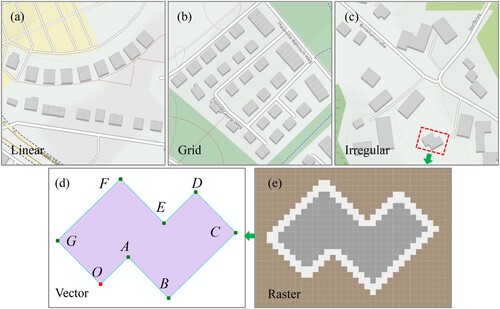
Vectors and rasters are two basic types of spatial data representations. Vector data apply the x and y coordinates to represent spatial information, which mainly includes three types of points, lines and polygons. For example, as shown in Figure 1d, a building can be represented using a start point O and a point set A-G. However, a raster consists of a pixel matrix with regular columns and rows, and each pixel contains a value used to represent spatial information. As shown in Figure 1e, the same building can be represented with a format of regular pixels. Although many vector-based methods for building typification have been developed, raster-based methods have received less attention. Furthermore, with the development of artificial intelligence, an increasing number of scholars have taken raster data as the basic object during the multiscale representation of spatial data. These scholars have applied neural networks (Feng, Thiemann, and Sester 2019; Kang, Gao, and Roth 2019) and computer vision technologies (Shen, Ai, and He 2018a; Shen et al. 2018b) for map generalization and representation. Thus, in this article, we develop a superpixel-based typification method for raster buildings with different distribution patterns, such as linear, grid and irregular patterns, using related computer vision technologies.

This article is organized as follows. Section 2 presents the related work regarding building typification. Section 3 illustrates the typification methods for buildings with linear, grid and irregular patterns, which mainly include how to group, position and reconstruct buildings. In Section 4, buildings from both cities and countrysides in China are applied to perform typification, and the proposed superpixel building typification (SUBT) method is discussed and analysed. Section 5 describes the conclusions and future work.

2. Related work

In traditional building typification methods, scholars usually utilize vector data as basic processing objects. Some typical vector-based methods include mesh-based (Burghardt and Cecconi 2007; Gong and Wu 2018; Wang and Burghardt 2019), geometric (Bildirici and Aslan 2010; Bildirici et al. 2011), Gestalt theory (Regnauld 2001), self-organizing maps (Sester 2005), graph-based (Anders and Sester 2000; Anders 2005) and data matching (Li, Guo, and Liu 2005) methods. For example, Burghardt and Cecconi (2007) proposed a mesh-based method for building typification that achieves high-speed results that can be reproduced for real-time applications. In this method, building typification is divided into two steps: the positioning of buildings using Delaunay triangulation and the representation of buildings by orientation and size calculation. This mesh-based typification method was proven to effectively constrain the density of buildings and preserve basic geometrical characteristics, such as shape, semantics and direction. However, these investigators mainly used buildings with irregular patterns for experiments but ignored buildings with linear and grid pattern distributions. Subsequently, Gong and Wu (2018) and Wang and Burghardt (2019) proposed typification methods for buildings with grid and linear patterns, respectively, based on Delaunay triangulation. Based on Gestalt theory, Regnauld (2001) considered different criteria, such as density, size and shape, for grouping buildings and typified buildings by finding the minimum spanning tree. This method can produce fewer, larger and better spaced buildings than the original, and it can effectively maintain the original distribution characteristics. However, in their experiments, buildings with grid patterns were not further analysed. Considering a web mapping environment, Li, Guo, and Liu (2005) proposed an on-the-fly typification method for buildings based on data matching. This method mainly includes three steps: calculation of the building number, representation of the building shape, and calculation of the building size. In their experiment, buildings with linear distribution patterns were not discussed. Raster-based methods for building typification have received little attention. In addition to buildings, typification methods for other map elements, such as ditches (Sandro, Massimo, and Matteo 2011), drainage (Zhang 2007), and façade structures (Shen et al. 2016), have also been proposed by various scholars.

Existing building typification methods usually need to detect the distribution patterns of buildings (Mesev 2005; Zhang et al. 2013; Du, Shu, and Feng 2016; He, Zhang, and Xin 2018). For example, Zhang et al. (2013) developed two algorithms for automatically identifying buildings with collinear and curvilinear patterns based on Delaunay triangulation and minimum spanning tree technologies. Du, Shu, and Feng (2016) proposed a relation-based method for detecting building patterns from three levels by defining 169 basic relations. He, Zhang, and Xin (2018) used machine learning and graph partitioning methods to recognize building patterns. This method was proven to have the ability to identify both regular and irregular patterns. In their method, the regular building pattern was divided into three types: rectangular, curvilinear and collinear patterns, and the irregular building pattern was divided into three types: high-density, H-shaped and L-shaped patterns.

The above analysis indicates that almost all methods for building typification are based on vector data, and it is rare to find raster-based methods for building typification. However, many kinds of raster map data exist, such as scanned maps and remote sensing image maps. When handling these raster maps, traditional vector-based generalization approaches usually require more human intervention, such as data format conversion and data quality correction of the vectorization of raster images, which is not conducive for preserving the data accuracy with respect to consistency and topological relations. Moreover, the vector data structure is complex, and there are numerous ways to categorize it, such as entity and topology type, which is not convenient for data standardization, normalization and exchange. Thus, to ensure the accuracy and versatility of map data during generalization based on raster data, raster-based generalization approaches are necessary. In addition, the existing typification method usually can handle only buildings with a single distribution pattern; thus, pattern recognition (Mesev 2005; Zhang et al. 2013; Du, Shu, and Feng 2016; He, Zhang, and Xin 2018) should always be applied before typification. However, in this paper, we develop a raster-based method for building typification considering distribution patterns. This method does not require the identification of any building patterns before typification but can effectively preserve the original distribution patterns, such as linear, grid and irregular patterns.

3. Methodologies for building typification

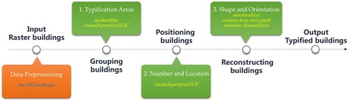
Basically, building typification can be summarized in one problem: transferring m buildings to n buildings, where $\mathrm{n}<\mathrm{m}$, while maintaining the original characteristics as much as possible. During this process, three basic problems should be solved: (1) determining the buildings with relatively close distances in typification areas that should be grouped for further typification; (2) determining the number and position of buildings; and (3) determining the geometrical patterns of the buildings, including size, orientation and shape. Thus, in this paper, the methodologies for building typification are divided into three corresponding tasks: grouping buildings with connected component detection and superpixel analysis, positioning buildings using second segmentation and reconstructing buildings using multiple strategies. A flow diagram of the proposed SUBT algorithm can be found in Figure 2, in which the italic text marked in yellow represents the main calculation functions of the OpenCV software library used to realize the corresponding steps.

Figure 2. Flow diagram of the proposed SUBT algorithm.

3.1. Grouping buildings with connected component detection and superpixel analysis

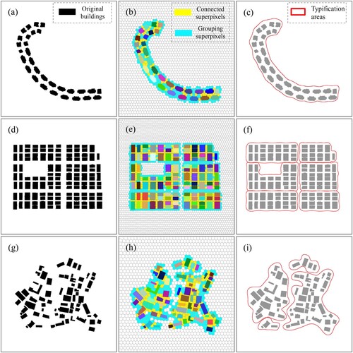
In raster data, building information is discrete. Thus, before grouping, the connected components corresponding to each building should be detected first. The detailed process for grouping buildings can be divided into the following three steps. The patterns of buildings can be divided into linear, grid and irregular (unstructured) patterns (Zhang et al. 2013). To better display the proposed method, a simple example is presented in Figure 3. The raster building data in this figure are generated from regular vector data, and we used the ‘Polygon to Raster’ toolbox in ArcGIS to convert vector data to raster data. The cell size used for rasterization is 0.3 meters per pixel. Figures 3(a, d and g) show the raster building data with linear, grid and irregular patterns. After the conversion of the data format, the original sizes of these three images are $1156\times 1156$ pixels.

Figure 3. Groupings of buildings.

3.1.1. Detection of connected components

There are two types of connected components: four-connected and eight-connected components. If only the edges of pixels touch, then they are four-connected components. If the edges or corners of pixels touch, then they are eight-connected components. Many scholars have proposed various algorithms for connected component labeling (Di Stefano and Bulgarelli 1999; Suzuki, Horiba, and Sugie 2003; He et al. 2009; Grana, Borghesani, and Cucchiara 2010). In this paper, the typical method for four-connected component labeling proposed by Haralick and Shapiro (1992) is applied. Figures 3(b, e and h) show the labeled connected components of buildings using pseudocolour. Using connected component labeling, the original discrete pixels are built as multiple objects.

3.1.2. Grouping using superpixel analysis

In the field of map generalization, superpixel technology was first applied to simplify polygonal and linear features (Shen et al. 2018b), and the authors analysed the similarities and differences between superpixel segmentation and map generalization. Subsequently, superpixel technology has been applied to building aggregation (Shen et al. 2019a), building simplification (Shen, Ai, and Li 2019b) and collapse (Shen, Ai, and Yang 2019c). Following this direction, in this paper, superpixel technology was applied to another important generalization operator: typification. After performing connected component labeling, superpixel segmentation algorithms are used for grouping. To generate relatively regularly shaped superpixels without manually setting the compactness parameter, the zero version of the simple linear iterative clustering (SLICO) method (Achanta et al. 2012) is applied. Compactness, which is the ratio of the perimeter to the area of the object, is used to measure the shape of an object. As shown in Figure 3(e, b and h), the superpixel sizes used for the first segmentation are 20, 25 and 30 pixels, respectively. The generated superpixel tends to have a hexagonal shape in blank regions, and it presents slight shape changes in building regions. When the boundary of a superpixel and the boundary of a building connected component overlap, this superpixel and building connected component are connected. When a superpixel (marked in yellow) generated by the first segmentation connects two or more connected components of buildings, these connected components will be grouped. In Figure 3, after grouping via superpixel analysis, the linear buildings are divided into one group, the grid buildings are divided into six groups, and the irregular buildings are divided into four groups.

3.1.3. Construction of the typification area

This step aims to establish the specific areas used for further typification. The new positions, number and shape of buildings will be calculated in these so-called typification areas. The typification areas are first made up of the connected components (marked in pseudocolour) and superpixels (marked in yellow and blue) used for grouping. Then, the edges of typification areas are smoothed to generate the final typification areas. Figures 3(c, f and i) show the final typification areas (outlined by the solid red lines) of buildings with linear, grid and irregular patterns.

3.2. Positioning buildings using second segmentation

In this step, the number and location of new typified buildings at different levels of detail will be determined by a second segmentation procedure. In this process, the typification areas (marked in light gray in Figure 4) will be segmented multiple times by larger superpixels to generate various levels of detail. For example, in Figure 4, for three types of buildings (linear, grid and irregular), the segmentation results at two levels of detail are generated. In Figures 4(a and b), the superpixel sizes that are used for the second segmentation of linear buildings are 150 and 230 pixels, respectively. In Figures 4(c and d), the superpixel sizes that are used for the second segmentation of grid buildings are 180 and 300 pixels, respectively. In Figures 4(e and f), the superpixel sizes that are used for the second segmentation of irregular buildings are 185 and 210 pixels, respectively. The number of new typified buildings at different levels of detail equals the number of superpixels generated by the second segmentation procedure.

Figure 4. Positioning the buildings.

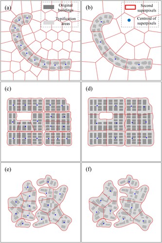
Then, the center of mass of each superpixel generated from the second segmentation is the new location typified from the original buildings located inside this superpixel. In Figure 4, the blue points are the center of mass of each superpixel, from which we can see that with increasing superpixel size, fewer centers of mass of superpixels are generated, which means that in one superpixel, more buildings will be typified to one building. In addition, the distribution patterns of the buildings are still preserved. For example, the distribution of the center of mass generated from linear buildings is still linear (Figures 4(a and b)), the distribution of the center of mass generated from grid buildings is still a grid (Figures 4(c and d)), and the distribution of the center of mass generated from irregular buildings is still irregular (Figures 4(c and d)).

In addition, two problems should be emphasized. First, we define a judgement rule R, namely, when a building falls into two or more adjacent superpixels, this building always belongs to the superpixel that has the most overlap with the building. Second, the typification areas defined in Section 3.1 should be separately extracted, and superpixel segmentation should be performed rather than segmenting all typification areas as a whole in one image during the second segmentation procedure. For example, in Figure 4f, there are four typification areas marked with red boundaries. In this case, each typification area will be separately extracted, and superpixel segmentation will be performed.

3.3. Reconstructing buildings using multiple strategies

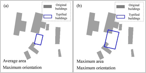
To reconstruct the typified buildings in the typification areas, three key parameters, namely, elongation, orientation and area, should be determined according to the following rules.

(1) Elongation. The elongation of new typified buildings can be calculated by the following equation: $E={\displaystyle \frac{L_{major}}{L_{minor}}}$

where $L_{major}$ is the length of the major axis of the minimum bounding rectangle of the building with the maximum area and $L_{minor}$ is the length of the minor axis of the minimum bounding rectangle of the building with the maximum area.

(2) Orientation. The orientation of new typified buildings can be calculated by the following equation: $O={\alpha }_1{O}_1+{\alpha }_2{O}_2+\cdots +{\alpha }_n{O}_n,({\alpha }_1+{\alpha }_2+\cdots {\alpha }_n=1)$

where ${\alpha }_1$,${\alpha }_2$,$\cdots$,${\alpha }_n$ are the weighting coefficients of the orientations of buildings $O_1$,$O_2$,$\cdots$,$O_n$ respectively, calculated using the image moment (Hu 1962). According to this equation, the multistrategy orientation calculation method is applied as follows.

Average orientation: when ${\alpha }_1={\alpha }_2=\cdots ={\alpha }_n$, the orientation O is the average orientation of the original buildings located inside the corresponding superpixel generated from the typification areas.

Maximum orientation: when one of the weighting coefficients equals 1. For example, if the area of building n is the maximum, then ${\alpha }_n=1$ and the orientation O equals the orientation of building $n$ with the maximum area.

Weighted orientation: when the weighting coefficients are not in the above two cases.

(3) Area. The area of new typified buildings can be calculated by the following equation: $A={\alpha }_1{A}_1+{\alpha }_2{A}_2+\cdots +{\alpha }_n{A}_n,({\alpha }_1+{\alpha }_2+\cdots {\alpha }_n=1)$

where ${\alpha }_1$,${\alpha }_2$,$\cdots$,${\alpha }_n$ are the weighting coefficients of the areas of buildings $A_1$,$A_2$,$\cdots$,$A_{\mathrm{n}}$, respectively. According to this equation, the multistrategy area calculation method is applied as follows.

Average area: when ${\alpha }_1={\alpha }_2=\cdots ={\alpha }_n$, area A is the average area of the original buildings located inside the corresponding superpixel generated from the typification areas.

Maximum area: when one of the weighting coefficients equals 1. For example, if the area of building n is the maximum, then ${\alpha }_n=1$ and area A equals the area of building $n$ with the maximum area.

Weighted area: when the weighting coefficients are not in the above two cases.

When area A is determined using the multistrategy area calculation method, a readjustment of the area can be performed. The dilation operation can be used to uniformly increase the area. During the dilation operation, the buildings should be first rotated with respect to the horizontal direction, and then the rectangular structure element should be applied. To avoid intersection, the maximum area after readjustment should be below the area of the corresponding superpixels generated from typification areas. In actual experiments, the related calculations, including the minimum bounding rectangle, image moment and basic geometric property, and drawing of typified results can be realized using the corresponding OpenCV functions.

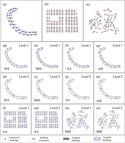
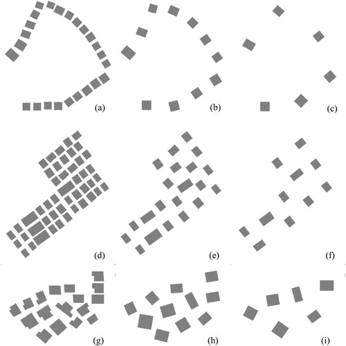
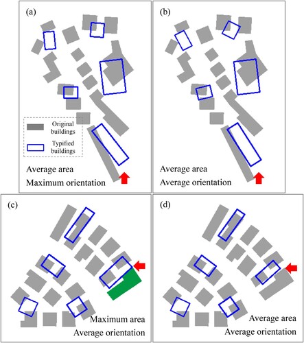
In Figure 5, various reconstruction strategies of typified buildings are performed. Figures 5(a, b and c) show the orientations of all original buildings. Figures 5d–k show the typified results of buildings with linear patterns using the maximum area and average orientation (MA), maximum area and maximum orientation (MM), average area and average orientation (AA), and average area and maximum orientation (AM) strategies at two different levels of detail; Figures 5(l and m) show the typified results of buildings with grid patterns using the AA strategy at two different levels of detail; and Figures 5(n and o) show the typified results of buildings with irregular patterns using the MM strategy at two different levels of detail. The blue buildings are the final typified buildings using the proposed method. The results show that the proposed method can effectively perform building typification while preserving the original linear, grid and irregular distribution patterns.

Figure 5. Reconstructed buildings.

4. Experiments and evaluations

Since we need to test whether the proposed SUBT method can be applied to address buildings with different distribution patterns, such as linear, grid and irregular patterns, the principle for selecting experimental areas is to determine whether they contain enough buildings with these three types of distribution patterns. Thus, two different sets of building data from cities and countrysides in China are selected, in which the former mainly contains buildings with linear grid patterns, while the latter mainly contains buildings with irregular patterns. Different typification strategies are applied in these two different sets of building data. The original building data originate from the Gaode map of China. The Gaode map can provide tile map services. Thus, the original data can be downloaded from the internet for free according to the corresponding uniform resource locator (Zhou et al. 2019). To generate the final regular experimental data used to test the proposed SUBT method, we performed a series of automatic and manual data processing operations, including preliminary extraction according to the color values, building simplification and aggregation, and transformation of building data format using ArcGIS software.

4.1. Typification of building data from the city

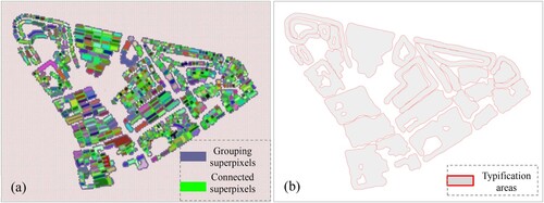
In this experiment, the city building data originate from the city of Shanghai in China. Because more attention is given to architecture planning in cities, the building distribution is more regular. The west longitude extent of the experimental building data is between 121.360 and 121.377 degrees, and the north latitude extent of the experimental building data is between 31.192 and 31.202 degrees. Figure 6a shows the original building data. After data format conversion with a cell size of 0.5 meters per pixel, the size of the final raster data is $3948\times 2950$ pixels. A total of 703 buildings are located in this experimental area. Most of these buildings form linear and grid patterns. Figure 7a shows the results of the grouping of buildings using superpixel analysis, and 30 building groups were generated. The corresponding construction result of 30 typification areas is shown in Figure 7b. The superpixel size of the first segmentation used for generating typification areas is ${\mathrm{S}}_1=23$.

Figure 6. Typification of building data from the city.

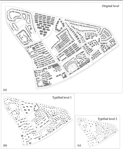
Figure 7. Grouping of the buildings and construction of the typification area.

Since the number of SLIC superpixels depends on the shape and resolution of buildings, a specified number of superpixels cannot be generated by setting a fixed superpixel size. However, a target map scale within a threshold range can be calculated according to Töpfer’s radical law (Töpfer and Pillewizer 1966): $S_{Tar}=S_{Ori}/{\left({\displaystyle \frac{N_{Tar}}{N_{Ori}}}\right)}^2$

In this equation,$S_{Tar}$ and $S_{Ori}$ are the denominators of the target and original map scales, respectively, and $N_{Tar}$ and $N_{Ori}$ are the number of buildings at the target and original map scales, respectively. The original scale of the building data is 1:5000. According to the generated number of buildings in Table 1, the corresponding display scales of the typification results at two levels are 1:20000 and 1:60000. The superpixel sizes of the second segmentation used for positioning buildings at two levels are ${\mathrm{S}}_2=90$ and ${\mathrm{S}}_2=120$. During typification, the two special cases for large buildings should be handled separately.

Table 1. Influences of various numbers of dilation operations on geometric changes of buildings during typification.

Scale	Number of Dilations	Area	Perimeter	Number
Original		1366262.00	145600.10	703
Level 1	0	786762.00 (↓ 42.4%)	72243.60 (↓ 50.3%)	352 (↓ 49.9%)
	1	884968.00 (↓ 35.2%)	74537.37 (↓ 48.8%)
	2	972747.00 (↓ 28.8%)	77637.22 (↓ 46.7%)
Level 2	0	522903.00 (↓ 61.7%)	45264.34 (↓ 68.9%)	215 (↓ 69.4%)
	1	579826.00 (↓ 57.6%)	47131.60 (↓ 67.6%)
	2	638010.00 (↓ 53.3%)	48827.60 (↓ 66.5%)

The first problem is the handling of local abnormally large buildings according to the following optional typification strategies, which are designed for preserving the global uniformity of the distribution of typified buildings.

(1) Strategy for merging superpixels. Assuming that $N_x$ is the number of buildings that belong to the same superpixel x after the judgement of rule R defined in Section 3.2, then $N_x\ge 0$.

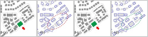
When a single building falls into two different superpixels A and B and the number of buildings contained in superpixels A and B equals 1, namely, $N_A+N_B=1$, these two superpixels A and B can be merged into a single superpixel. An example can be found in Figure 8. The building marked in blue falls into two superpixels that do not contain any other buildings after the area calculation decides which buildings belong in the superpixels. Thus, these two superpixels can be merged into one superpixel, the corresponding number of typified buildings decreases by one, and the number of centers of mass is reduced from two (marked in red in Figure 8a) to one (marked in blue in Figure 8c). As shown in Figure 8b, when this merging strategy is not applied, the location of the typified building has a larger displacement that affects the uniformity of the global distribution of buildings. Using this strategy, the global uniformity of the distribution of typified buildings can be well preserved, as shown in Figure 8d.

Figure 8. Strategy for merging superpixels.

(2) Strategy for building decomposition. When a single building falls into three or more different superpixels A, B, C, $\cdots$, and the number of buildings contained in these superpixels A, B, C, $\cdots$ equals 1, namely, $N_A+N_B+N_C+\cdots =1$, this building can be divided into several parts by the superpixels. An example can be found in Figure 9. Figure 9a shows an example of the original building data. After a second segmentation procedure, the building marked in red falls into three superpixels, and there are no other redundant buildings that fall into these three superpixels. Thus, this building can be optionally divided into three parts (marked in green in Figure 9b) according to the boundaries of the three superpixels. Figures 9b and 9c show the typified results with and without the strategy of building decomposition, respectively. Using this typification strategy, the original building distribution pattern can be well preserved.

Figure 9. Strategy for building decomposition.

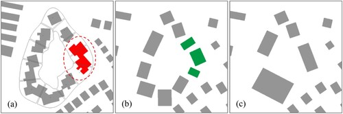
The second problem is the avoidance of intersections. Sometimes, adjacent typified buildings may generate intersections. Thus, the erosion operation can be applied. During the process of erosion, to maintain the orthogonal characteristics of the typified buildings, the buildings should first be rotated with respect to the horizontal direction. Then, the rectangular structure element used for erosion should be applied. Finally, the buildings should be rotated to the original direction. An example can be found in Figure 10. Figure 10a shows the original buildings and the red typification areas. Figure 10b shows the typified results with a building intersection. Figure 10c shows the typified buildings after the erosion operation, from which we can see that the building marked in orange is shrunk to the inside of the corresponding superpixel. For some long and narrow buildings, erosion operations may lead to the disappearance of buildings. In this case, the buildings should gradually adjust their length and width while preserving the original area to avoid intersections.

Figure 10. Avoidance of intersections.

Since most buildings in the experimental area form linear and grid patterns, the optional typification strategies, the average area and average orientation typification strategies are applied to the building data from Shanghai.

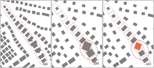
Figure 11 shows some typical examples of building typification at two different levels, from which we can see that when buildings positioned linearly along the roads are typified, the original linear pattern can be well preserved at two different levels of detail, as shown in Figures 11a–c. When the grid buildings are typified, the original grid pattern can be well preserved at two different levels of detail, as shown in Figures 11d–f. When irregular buildings are typified, the original distribution patterns can be preserved well, as shown in Figures 11g–i.

Figure 11. Typical examples of building typification at two levels.

To evaluate the validity of the typification model, the inconsistency before and after typification (Gong and Wu 2018) can usually be measured by geometry changes. We analysed the influences of various numbers of dilation operations on geometric changes of buildings during typification, which can be found in Table 1. From Table 1, without the dilation operation for enlarging typified buildings and with an increasing level, the reduction in the area (from 42.4% to 61.7%), perimeter (from 50.3% to 68.9%) and number of buildings (from 49.9% to 69.4%) increases. When the dilation operation is applied to enlarge the typified buildings at level 1 and the number of dilations increases, the reduction in the area (from 35.2% to 28.8%) and the perimeter (from 48.8% to 46.7%) decreases. When the dilation operation is used to enlarge the typified buildings at level 2 and the number of dilations increases, the reduction in the area (from 57.6% to 53.3%) and the perimeter (from 67.6% to 66.5%) decreases. Compared with level 1, level 2 has a more reduced area and perimeter because of the reduction in the number of buildings.

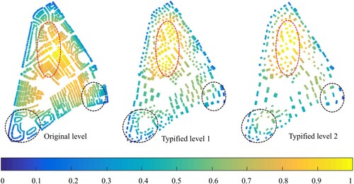
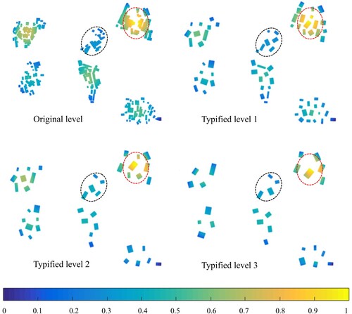
The relative distribution density of buildings calculated by overlaying circles with a certain area centered at each pixel point from the city before and after typification can be found in Figure 12. The yellow and blue parts represent high- and low-density areas, respectively. Compared with the original distribution density, the overall relative distribution density trends at the two typified levels are generally consistent. The high-density areas still tend to have a high density, and the low-density areas still tend to have a low density, as shown in the relatively high-density regions marked with red ellipses and the relatively low-density regions marked with black ellipses.

Figure 12. Density comparison before and after typification.

To quantifiably compare the relative density before and after typification, we counted the average density of all typification areas in Figure 7 according to the density level of each pixel that consists of buildings. Assuming that d is the relative density value, we divided the average density values into three levels: high ($0.70\le \mathrm{d}\le 1.0$), middle ($0.3<\mathrm{d}<0.7$) and low ($0\le \mathrm{d}\le 0.3$). We counted the numbers and percentages of typified areas that possessed the same density level between the original and typified scales to measure the changes in relative distribution density. The density consistency information can be found in Table 2, which shows that the percentages of consistent density at the two typification levels are up to 86.7% and 90.0%, which means that the relative distribution density is well maintained during typification.

Table 2. Relative density consistency information at two different levels.

	Consistent high density	Consistent middle density	Consistent low density	Consistent density	Inconsistent density
Level 1	8 (26.7%)	17 (56.7%)	1 (3.3%)	26 (86.7%)	4 (13.3%)
Level 2	8 (26.7%)	18 (60.0%)	1 (3.3%)	27 (90.0%)	3 (10.0%)

Some typical examples of typification using various area and orientation strategies can be found in Figure 13. In Figure 13, the gray buildings are the original buildings, and the blue buildings are the typified buildings. Figures 13(a and b) show the typification results using the average area and the maximum orientation strategies and the average area and average orientation strategies, from which we can see that the area, number and distribution of typified buildings in these two subfigures are the same, while only the orientation is different, as marked with the red arrow. In cartography, when a building is very important, it may be emphatically displayed. For example, if the building marked in green in Figure 13c is Jin Mao Tower in Shanghai, which is a landmark building, then the typification strategy of the maximum area used in Figure 13c is better than the typification strategy of the average area used in Figure 13d. Using the multistrategy typification procedure, the semantic feature can be well considered, and cartography options can be flexibly and conveniently provided.

Figure 13. Typification using different strategies.

4.2. Typification of building data from the countryside

In this experiment, the countryside building data are from the suburbs of Wuhu City in China. Because less attention is usually given to architecture planning in the suburbs, the building distribution is more irregular. The west longitude extent of the experimental building data is between 118.412 and 118.422 degrees, and the north latitude extent of the experimental building data is between 31.400 and 31.412 degrees.

Figure 14 shows the original building data. After data format conversion with a cell size of 0.5 meters per pixel, the size of the final raster data is $2856\times 2368$ pixels. There are a total of 142 buildings in this experimental area. Most of these buildings form irregular patterns. Figure 15a shows the results of grouping the buildings using superpixel analysis, and 6 building groups were generated. The corresponding construction result of the 6 typification areas is shown in Figure 15b. The superpixel size of the first segmentation used for generating typification areas is ${\mathrm{S}}_1=50$. The original scale of the building data is 1:5000. According to Töpfer’s radical law and the generated number of buildings in Table 3, the corresponding display scales of the typification results at three levels are 1:20000, 1:60000 and 1:120000. The superpixel sizes of the second segmentation used for positioning buildings at three levels are ${\mathrm{S}}_2=130$, ${\mathrm{S}}_2=180$ and ${\mathrm{S}}_2=230$.

Figure 14. Original experimental buildings from the countryside.

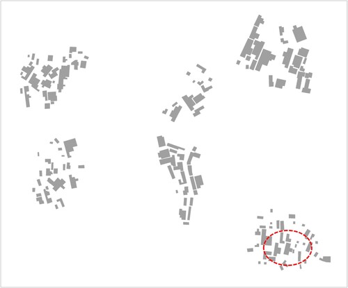
Figure 15. Grouping of buildings and construction of the typification areas.

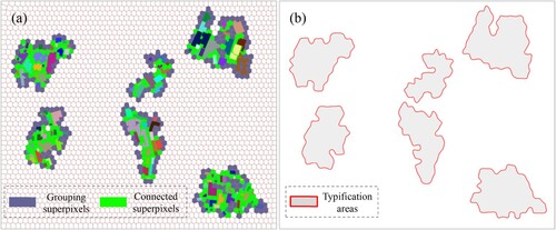
Table 3. Influences of various numbers of dilation operations on geometric changes of buildings during typification.

Scale	Number of Dilation	Area	Perimeter	Number
Original		357306.00	35966.94	142
Level 1	0	280852.00 (↓ 21.4%)	19393.69 (↓ 46.1%)	71 (↓ 50.0%)
	1	311032.00 (↓ 13.0%)	19643.00 (↓ 45.4%)
	2	334094.00 (↓ 6.5%)	20121.46 (↓ 44.1%)
Level 2	0	229845.00 (↓ 35.7%)	13079.57 (↓ 63.6%)	42 (↓ 70.4%)
	2	261439.00 (↓ 26.8%)	13798.79 (↓ 61.6%)
	4	294307.00 (↓ 17.6%)	14470.79 (↓ 59.8%)
Level 3	0	197108.00 (↓ 44.8%)	10112.44 (↓ 71.9%)	29 (↓ 79.6%)
	4	246838.00 (↓ 30.9%)	11074.41 (↓ 69.2%)
	6	273078.00 (↓ 23.6%)	11538.41 (↓ 67.9%)

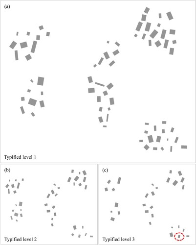
Figures 16(a, b and c) show the typified buildings at these three levels using the maximum area and maximum orientation strategies, from which we can see that the proposed method can effectively realize the typification of buildings with irregular distribution patterns. As the level increases, the number of original groupings deceases, and the original irregular distribution patterns can be well preserved.

Figure 16. Typification of building data from the countryside.

The influences of various numbers of dilation operations on geometric changes of buildings during typification can be found in Table 3. From Table 3, without dilation for enlarging typified buildings and with an increasing level, the reduction in the area (from 21.4% to 44.8%), perimeter (from 46.1% to 71.9%) and number of buildings (from 50.0% to 79.6%) increases. When the dilation operation is used to enlarge the typified buildings at level 1 and the number of dilations increases, a reduction in the area (from 13.0% to 6.5%) and perimeter (from 45.4% to 44.1%) decreases. When the dilation operation is used to enlarge the typified buildings at level 2 and the number of dilations increases, the reduction in the area (from 26.8% to 17.6%) and perimeter (from 61.6% to 59.8%) decreases. When the dilation operation is used to enlarge the typified buildings at level 3 and the number of dilations increases, the reduction in the area (from 30.9% to 23.6%) and perimeter (from 69.2% to 67.9%) decreases. With increasing levels, the area and perimeter decrease because of the reduction in the number of buildings.

Compared with the experimental results of city building data, the area change at the same typified level 1 using the building data from the suburbs of Wuhu (13.0% and 6.5%) is observably less than that from the city of Shanghai (35.2% and 28.8%), even if the same number of dilations were used. This finding is because the typification strategy used for the building data of Shanghai is the average area and the typification strategy used for the building data of Wuhu is the maximum area. As shown in Figure 17, the subregion comes from the original data marked in the red circle. The area differences between the individual buildings are relatively large. Additionally, the average area strategy leads to a relatively large reduction in the area, whereas the maximum area strategy leads to a relatively small reduction in the area.

Figure 17. Typification using different strategies.

The relative distribution density of buildings from the countryside before and after typification can be found in Figure 18. The yellow and blue parts represent high- and low-density areas, respectively. Compared with the original distribution density, the overall relative density distribution trends at the three typified levels are generally consistent, as shown in the relatively high-density regions marked with red ellipses and the relatively low-density regions marked with black ellipses.

Figure 18. Density comparison before and after typification.

The density consistency information during typification can be found in Table 4, which shows that the percentages of consistent building density at three typification levels are up to 100%, 83.3% and 83.3%. Although the density levels of the buildings in one typification area are inconsistent at levels 2 and 3, the corresponding average density values are all approximately 0.3, and the density differences between the typified and original buildings in the typification area at both levels are less than 0.15, which means that the relative distribution density is well maintained during typification.

Table 4. Relative density consistency information at three different levels.

	Consistent high density	Consistent middle density	Consistent low density	Consistent density	Inconsistent density
Level 1	0 (0%)	6 (100.0%)	0 (0%)	6 (100.0%)	0 (0%)
Level 2	0 (0%)	5 (83.3%)	0 (0%)	5 (83.3%)	1 (16.7%)
Level 3	0 (0%)	5 (83.3%)	0 (0%)	5 (83.3%)	1 (16.7%)

4.3. Comparison with the vector-based typification method

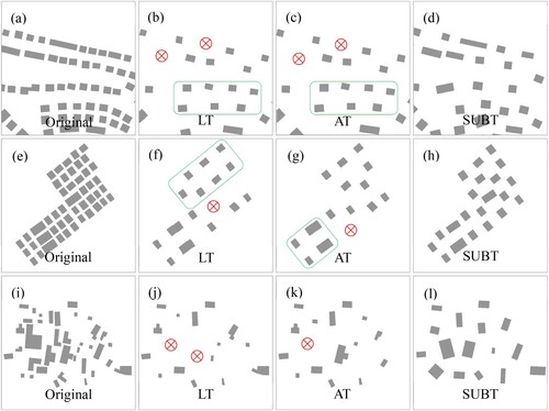
To show the advantages of the proposed raster-based SUBT method, we compared it with a vector-based generic building typification method proposed by Bildirici et al. (2011). Although some other typification methods have been proposed in recent years, such as the methods proposed by Gong and Wu (2018) and Wang and Burghardt (2019), they have strict requirements in terms of regular spatial patterns and are limited to certain fixed patterns, such as linear (Gong and Wu 2018) and grid (Wang and Burghardt 2019) patterns, making them less comparable to our method than the method proposed by Bildirici et al. (2011). In Bildirici’s method, a length typification method (LT) and an angle typification (AT) method are developed for generic buildings, which can maintain the shape and coverage of building groups. Figure 19 shows the comparisons of typification results between vector-based LT and AT methods and the proposed raster-based SUBT method. The original buildings are displayed in Figures 19(a, e and i). Although the vector-based LT and AT methods can generate encouraging results in different cases, as shown in the regions marked with green boxes in Figures 19(b–c and f–g), they tend to result in gaps among building groups, such as the regions marked with red cross-shape labels in Figures 19(b–c, f–g and j–k), and the original spatial distribution pattern, such as linear, grid and irregular patterns, cannot be well preserved. However, the proposed raster-based SUBT method can effectively avoid generating gaps and maintain the original spatial distribution patterns, such as the linear, grid and irregular patterns in Figures 19(d, h, and l).

Figure 19. Comparisons between the vector-based and proposed raster-based SUBT methods.

We also quantifiably compare and analyse the vector-based LT and AT methods and raster-based SUBT method. The evaluation indicator used to measure the inconsistency before and after typification (Gong and Wu 2018) can be calculated as follows: ${\mathrm{R}}_{\mathrm{x}}=\left|({\mathrm{I}}_{\mathrm{B}}^{\mathrm{x}}-{\mathrm{I}}_{\mathrm{A}}^{\mathrm{x}})/{\mathrm{I}}_{\mathrm{B}}^{\mathrm{x}}\right|$

where ${\mathrm{I}}_{\mathrm{B}}^{\mathrm{x}}$ denotes the xth indicator value in indicator set I before typification and ${\mathrm{I}}_{\mathrm{A}}^{\mathrm{x}}$ denotes the xth indicator value in indicator set I after typification. The lower the ${\mathrm{R}}_{\mathrm{x}}$ value is, the better the consistency and the better the typification results. In this study, set I contains three indicators, namely, sum area, global distribution density and range (Wang et al. 2017; Gong and Wu 2018).

The comparison results of these three indicators between the vector-based (LT and AT) and proposed raster-based SUBT methods can be found in Table 5, from which we can see the following. First, the area changes during typification generated from the SUBT method are significantly lower than those of the vector-based LT and AT methods. For example, at level 1 for the typification of buildings from the countryside, the area changes of LT and AT are 0.611 and 0.500, respectively, while the area change of the SUBT method is only 0.065. This is mainly because the SUBT applies the dilation operation to reduce area changes. Second, the differences in density changes between the vector-based (LT and AT) and raster-based SUBT methods are not very large, while the latter performs better. For example, at level 1 in the typification of buildings from the city, the density changes of LT and AT are 0.536 and 0.617, respectively, which is less than ten percent larger than that of the SUBT method. Finally, the differences in range changes between the vector-based (LT and AT) and raster-based SUBT methods are close. Sometimes, the range changes of SUBT are slightly higher than those of the vector-based method. For example, at level 1 for the typification of buildings from the countryside, the range change of LT is 0, while the range change of the SUBT method is 0.002. Sometimes, the range changes of SUBT are slightly lower than those of the vector-based method. For example, at level 1 for the typification of buildings from cities, the range change of AT is 0.016, while the range change of the SUBT method is 0.001.

Table 5. Comparisons of changes in sum area, global distribution density and range between the vector-based (LT and AT) and proposed raster-based SUBT methods.

Methods	Village	Area changes	Density changes	Range changes	City	Area changes	Density changes	Range changes
LT	1	0.611	0.556	0	1	0.552	0.536	0.033
	2	0.732	0.609	0.154	2	0.636	0.626	0.003
	3	0.815	0.712	0.145
AT	1	0.500	0.549	0.078	1	0.585	0.617	0.016
	2	0.598	0.634	0.114	2	0.724	0.732	0.015
	3	0.705	0.726	0.228
SUBT	1	0.065	0.501	0.002	1	0.288	0.501	0.001
	2	0.176	0.643	0.172	2	0.533	0.687	0.022
	3	0.236	0.712	0.292

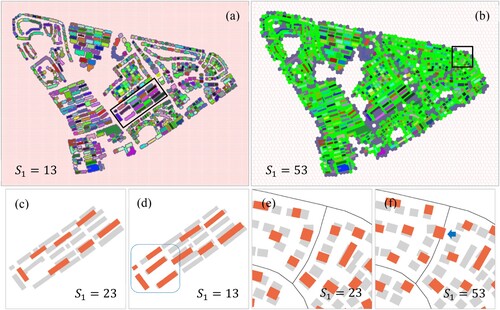
4.4. Parameter settings and strategy selection

There are two main parameters in the proposed SUBT method: the superpixel size ($S_1$) of the first segmentation used for generating typification areas and the superpixel size ($S_2$) of the second segmentation used for positioning buildings. The parameter $S_1$ has a decisive influence on the result of building grouping. When $S_1$ is too small, it cannot generate sufficiently large typification areas and is unable to achieve the effect of typification. For example, Figures 20(a and b) show the grouping results of original buildings using a small $S_1=13$ and a large $S_1=53$, respectively, while the appropriate grouping results can be found in Figure 7a when $S_1=23$. Figures 20c–f show the contrasting results of typification using these three values. When ${\mathrm{S}}_1$ is too small, such as $S_1=13$, some scattered buildings cannot be effectively typified, such as the buildings marked with blue boxes in Figure 20d, while this phenomenon can be avoided when $S_1=23$, as shown in Figure 20c. When $S_1$ is too large, it may cause the overlapping of buildings and other geographical elements, such as main roads. For example, in Figure 20f, when $S_1=53$, the typified building marked with a blue arrow overlaps with the main road, while a suitable value can avoid overlapping phenomena, such as the typified results in Figure 20e when $S_1=13$. For the parameter $S_2$, its size can be determined according to Töpfer’s radical law described in Section 4.1. For a given target scale, a corresponding fixed superpixel size $S_2$ can be automatically determined to obtain the corresponding number of typified buildings.

Figure 20. Impact of parameter settings on the typification results.

In actual applications, when setting the parameters $S_1$ and $S_2$, we recommend the following rules. Assuming that $w_{\mathrm{a}}$ is the width of the main road, $w_{\mathrm{b}}$ is the width of a secondary road one grade below the main road, $A_{\mathrm{t}}$ is the area of all typification regions, where $w_{\mathrm{a}}$, $w_{\mathrm{b}}$ and $A_{\mathrm{t}}$ are defined in units of pixels, $S_{Tar}$ and $S_{Ori}$ are the denominators of the target and original map scales, respectively, and $N_{Ori}$ is the number of buildings at the original map scale, then, the preliminary parameter values of $S_1$ and $S_2$ can be set as follows: $w_b^2<T_1<w_a^2,S_1=\sqrt{T_1}$ $T_2={\displaystyle \frac{A_t}{N_{Ori}\times \sqrt{S_{Tar}/S_{Ori}}},S_2=\sqrt{T_2}}$

To obtain a satisfactory typification result, we can fine-tune these preliminary values of $S_1$ and $S_2$. The rules for setting the values of $S_1$ and $S_2$ are not applicable in all cases, especially in the case of isolated buildings.

In the proposed SUBT method, we designed different typification strategies. In the countryside, since the construction of buildings is not uniformly planned, the size of the building area varies greatly. If the average area strategy is used, there will be a great visual difference. That is, there are obviously large buildings in the building group, but the typification building is very small, such as the typified results in Figure 17a. In this case, the maximum area strategy is selected. In cities, since the construction of buildings is usually uniformly planned, the changes in building area or orientation are small. In this case, the average strategy is a better choice because it can represent an average level of area or orientation for a cluster of buildings while maintaining a good visual effect. However, it is not a mandatory step to distinguish city buildings from countryside buildings since the typification strategies are mainly recommended to obtain better typification results. According to this principle, we provide the following recommendations for selecting typification strategies when using the proposed SUBT method.

• If there are small area differences between buildings, the average area strategy is recommended.

• If there are small orientation differences between buildings, the average orientation strategy is recommended.

• If there are large area differences between buildings, the maximum area strategy is recommended.

• If there are large orientation differences between buildings, the maximum orientation strategy is recommended.

In addition, these strategies can be used flexibly according to different cartography scenarios. For example, the average area strategy may be a better choice if the maximum area strategy causes many overlaps with other map elements.

5. Conclusions

This study proposes an innovative approach for building typification. The existing typification method can usually handle only buildings with a single distribution pattern; thus, building pattern recognition is required. However, our study focuses on the raster-based method for building typification using related computer vision technologies, in which different distribution characteristics can be well considered. In the proposed method, buildings with different distribution patterns, such as linear, grid and irregular patterns, are first grouped by image connected component detection and superpixel analysis. Then, the new positions of the buildings in the typification areas are calculated using a second segmentation procedure. Finally, a multistrategy representation of buildings is generated by the analysis of the orientation and shape of the buildings in the typification areas. The following conclusions can be drawn.

1. The proposed method can effectively realize multistrategy typification, such as the average and maximum orientation, the average and maximum area, and the strategy of building decomposition. Thus, the geometric and semantic features of buildings can be well considered, thus providing flexible options for cartography.

2. Compared with vector-based LT and AT typification methods, the proposed SUBT method performs better in preserving the distribution patterns (linear, grid and irregular), density and geometry features of buildings, while the distribution range cannot be maintained as well as the vector-based methods.

Some limitations and improvements of the proposed method should be mentioned. First, a second segmentation procedure is used in the proposed method, and many adjustments are required to determine the optimal segmentation parameters at different levels of detail. Thus, how to automatically determine the optimal segmentation parameters according to the size, direction and distribution of the original buildings is a further research direction. Second, during grouping, only geometric proximity is considered, and other aspects, such as semantic and directional features, should be considered. Moreover, scholars have also considered the shapes of typified buildings, such as L-shaped and U-shaped buildings (Stoter et al. 2010), during typification, while the proposed method cannot achieve these shapes. Finally, the topological relationships with roads, river systems and other elements are not fully considered in the proposed method. These relationships can be explored in the future.

Acknowledgement

This work was supported by the National Natural Science Foundation of China under Grant 42001402; the China Postdoctoral Science Foundation under Grant 2021M692464 and 2021T140521; the National Key Research and Development Program of China under Grant 2017YFB0503601 and 2017YFB0503502; the National Natural Science Foundation of China under Grant 41671448; Open Fund of Key Laboratory of Urban Land Resources Monitoring and Simulation, Ministry of Natural Resources; and the China Scholarship Council (CSC) under Grant 202006275019.

Data and codes availability statement

The experimental data are available at the following website: https://github.com/Cartography0706/BuildingTypification

Declaration of interests

The authors declare that they have no known competing financial interests or personal relationships that could have appeared to influence the work reported in this paper.

Disclosure statement

No potential conflict of interest was reported by the author(s).

Additional information

Funding

This work was supported by National Natural Science Foundation of China: [Grant Number 42001402]; China Postdoctoral Science Foundation: [Grant Number 2021T140521 and 2021M692464]; National Key Research and Development Program of China: [Grant Number 2017YFB0503601]; National Natural Science Foundation of China: [Grant Number 41671448]; Open Fund of Key Laboratory of Urban Land Resources Monitoring and Simulation, Ministry of Natural Resources; China Scholarship Council: [Grant Number 202006275019].

References

- Achanta, R., et al. 2012. “SLIC Superpixels Compared to State-of-the-art Superpixel Methods.” IEEE Transactions on Pattern Analysis and Machine Intelligence 34 (11): 2274–2282.
- Ai, T., S. Ke, M. Yang, and J. Li. 2017. “Envelope Generation and Simplification of Polylines Using Delaunay Triangulation.” International Journal of Geographical Information Science 31 (2): 297–319.
- Ai, T., X. Zhang, Q. Zhou, and M. Yang. 2015. “A Vector Field Model to Handle the Displacement of Multiple Conflicts in Building Generalization.” International Journal of Geographical Information Science 29 (8): 1310–1331.
- Anders, K. H. 2005. “Level of Detail Generation of 3D Building Groups by Aggregation and Typification.” Proceedings of the 22nd International Cartographic conference, coruña, Spain, 9–16 July 2005.
- Anders, K. H., and M. Sester. 2000. “Parameter-free Cluster Detection in Spatial Databases and its Application on Typification.” Int. Arch. Photogramm. Remote Sens 2000 (33): 75–83.
- Basaraner, M., and S. Cetinkaya. 2017. “Performance of Shape Indices and Classification Schemes for Characterising Perceptual Shape Complexity of Building Footprints in GIS.” International Journal of Geographical Information Science 31 (10): 1952–1977.
- Basaraner, M., and M. Selcuk. 2008. “A Structure Recognition Technique in Contextual Generalisation of Buildings and Built-up Areas.” The Cartographic Journal 45 (4): 274–285.
- Bildirici, I., and S. Aslan. 2010. “Building Typification at Medium Scales.” Proceedings of the 3rd International Conference on Cartography and GIS, nesebar, Bulgaria, 12–15 June.
- Bildirici, I., S. Aslan, O. Simav, and O. N. Çobankaya. 2011. “A Generic Approach to Building Typification.” Proceedings of the 14th ICA/ISPRS workshop on Generalisation and multiple representation, Paris, France, 30 June–1 July 2011; pp. 1–10.
- Burghardt, D., and A. Cecconi. 2007. “Mesh Simplification for Building Typification.” International Journal of Geographical Information Science 21 (3): 283–298.
- Cetinkaya, S., M. Basaraner, and D. Burghardt. 2015. “Proximity-based Grouping of Buildings in Urban Blocks: A Comparison of Four Algorithms.” Geocarto International 30 (6): 618–632.
- Change software. Hannover, Leibniz Universität Hannover. Available from: https://www.ikg.uni-hannover.de/en/service/software/change [Accessed 22 February 2020].
- Di Stefano, L., and A. Bulgarelli. 1999, September. “A Simple and Efficient Connected Components Labeling Algorithm.” Proceedings 10th International Conference on image analysis and Processing (pp. 322-327). IEEE.
- Du, S., M. Shu, and C. C. Feng. 2016. “Representation and Discovery of Building Patterns: A Three-Level Relational Approach.” International Journal of Geographical Information Science 30 (6): 1161–1186.
- Feng, Y., F. Thiemann, and M. Sester. 2019. “Learning Cartographic Building Generalization with Deep Convolutional Neural Networks.” ISPRS International Journal of Geo-Information 8 (6): 258.
- Gong, X., and F. Wu. 2018. “A Typification Method for Linear Pattern in Urban Building Generalisation.” Geocarto International 33 (2): 189–207.
- Grana, C., D. Borghesani, and R. Cucchiara. 2010. “Optimized Block-Based Connected Components Labeling with Decision Trees.” IEEE Transactions on Image Processing 19 (6): 1596–1609.
- Haralick, R. M., and L. G. Shapiro. 1992. “Computer and Robot Vision.” Addison-Wesley Volume I: 28–48.
- He, L., Y. Chao, K. Suzuki, and K. Wu. 2009. “Fast Connected-Component Labeling.” Pattern Recognition 42 (9): 1977–1987.
- He, X., X. Zhang, and Q. Xin. 2018. “Recognition of Building Group Patterns in Topographic Maps Based on Graph Partitioning and Random Forest.” ISPRS Journal of Photogrammetry and Remote Sensing 136: 26–40.
- Hu. K. 1962. “Visual Pattern Recognition by Moment Invariants.” IRE Trans.Inf. Theory 8 (2): 179–187. Feb.
- Kang, Y., S. Gao, and R. E. Roth. 2019. “Transferring Multiscale map Styles Using Generative Adversarial Networks.” International Journal of Cartography, 5, 1–27.
- Li, H., Q. Guo, and J. Liu. 2005. “Rapid Algorithm of Building Typification in web Mapping.” Proceedings of the International symposium on spatio-temporal modelling, spatial reasoning, analysis, data mining and data fusion, Beijing, China, 27–29 August 2005.
- Li, Z., H. Yan, T. Ai, and J. Chen. 2004. “Automated Building Generalization Based on Urban Morphology and Gestalt Theory.” International Journal of Geographical Information Science 18 (5): 513–534.
- Mesev, V. 2005. “Identification and Characterisation of Urban Building Patterns Using IKONOS Imagery and Point-Based Postal Data.” Computers, Environment and Urban Systems 29 (5): 541–557.
- Regnauld, N. 2001. “Contextual Building Typification in Automated map Generalization.” Algorithmica 30 (2): 312–333.
- Sandro, S., R. Massimo, and Z. Matteo. 2011. “Pattern Recognition and Typification of A. Ruas (Ed.), Ditches.” In Advances in Cartography and GIScience. Volume 1, 425–437. Berlin, Heidelberg: Springer.
- Sester, M. 2005. “Optimization Approaches for Generalization and Data Abstraction.” International Journal of Geographical Information Science 19 (8-9): 871–897.
- Shen, Y., T. Ai, and Y. He. 2018a. “A new Approach to Line Simplification Based on Image Processing: A Case Study of Water Area Boundaries.” ISPRS International Journal of Geo-Information 7 (2): 41.
- Shen, Y., T. Ai, and C. Li. 2019b. “A Simplification of Urban Buildings to Preserve Geometric Properties Using Superpixel Segmentation.” International Journal of Applied Earth Observation and Geoinformation 79: 162–174.
- Shen, Y., T. Ai, W. Li, M. Yang, and Y. Feng. 2019a. “A Polygon Aggregation Method with Global Feature Preservation Using Superpixel Segmentation.” Computers, Environment and Urban Systems 75: 117–131.
- Shen, Y., T. Ai, L. Wang, and J. Zhou. 2018b. “A new Approach to Simplifying Polygonal and Linear Features Using Superpixel Segmentation.” International Journal of Geographical Information Science 32 (10): 2023–2054.
- Shen, Y., T. Ai, and M. Yang. 2019c. “Extracting Centerlines from Dual-Line Roads Using Superpixel Segmentation.” IEEE Access 7: 15967–15979.
- Shen, J., H. Fan, B. Mao, and M. Wang. 2016. “Typification for Façade Structures Based on User Perception.” ISPRS International Journal of Geo-Information 5 (12): 239.
- Stoter, J., B. Baella, C. A. Blok, et al. 2010. State-of-the-art of Automated Generalisation in Commercial Software (p. 231). Dublin: EuroSDR.
- Suzuki, K., I. Horiba, and N. Sugie. 2003. “Linear-time Connected-Component Labeling Based on Sequential Local Operations.” Computer Vision and Image Understanding 89 (1): 1–23.
- Töpfer, F., and W. Pillewizer. 1966. “The Principles of Selection.” The Cartographic Journal 3 (1): 10–16.
- Wang, X., and D. Burghardt. 2019. “A Mesh-Based Typification Method for Building Groups with Grid Patterns.” ISPRS International Journal of Geo-Information 8 (4): 168.
- Wang, L., Q. Guo, Y. Liu, Y. Sun, and Z. Wei. 2017. “Contextual Building Selection Based on a Genetic Algorithm in map Generalization.” ISPRS International Journal of Geo-Information 6 (9): 271.
- Zhang, Q. 2007. “Drainage Typification Based on Dendritic Decomposition.” The Cartographic Journal 44 (4): 321–328.
- Zhang, X., T. Ai, J. Stoter, M. J. Kraak, and M. Molenaar. 2013. “Building Pattern Recognition in Topographic Data: Examples on Collinear and Curvilinear Alignments.” Geoinformatica 17 (1): 1–33.
- Zhou, X., T. Ai, N. Meng, and P. Xie. 2019. “A PDF Tile Model for Geographic Map Data.” ISPRS International Journal of Geo-Information 8 (9): 373.