Performances of six reanalysis profile products in the atmospheric correction of passive microwave data for estimating land surface temperature under cloudy-sky conditions

ABSTRACT

Passive microwave (PMW) observations from the Advanced Microwave Scanning Radiometer 2 provide a way to obtain cloudy land surface temperatures (LSTs). However, atmospheric corrections must be performed on cloudy LSTs due to the cloud effect at higher frequencies. In this paper, six reanalyzed profiles, including the fifth-generation European Centre for Medium-range Weather Forecasts Reanalysis (ERA5), Interim Reanalysis (ERA-Interim), Japanese 55-year Reanalysis Data (JRA-55), Modern-Era Retrospective analysis for Research and Application V2 (MERRA2), National Centers for Environmental Prediction (NCEP) /Final Operational Global Analysis (FNL), and NCEP/Global Forecasting System (GFS), were compared with 2829 radiosonde profiles derived from the University of Wyoming. Then, their performances in correcting the atmospheric effects of LSTs at cloudy skies were investigated. Results showed that the ERA5 had the best accuracy in revealing the actual atmospheric conditions, and the RMSEs of transmittance, downward radiance, and upward radiance were about 0.007, 2.01, and 1.89 K, respectively. The RMSEs between the estimated LSTs and referenced LSTs varied from 3.15 K of the ERA5 to 6.12 K of the NCEP/FNL, indicating the ERA5 can be recommended for the atmospheric correction of PMW-based LST retrievals. Additionally, transmittance accuracy plays an essential role in impacting the LST retrievals in any weather.

KEYWORDS:

• Reanalysis product
• land surface temperature
• atmospheric correction
• AMSR2
• evaluation

1. Introduction

The land surface temperature (LST) is a very critical biophysical surface variable in the surface energy and water balances between the atmosphere and the ground over regional and global scales (Anderson et al. 2008; Kustas and Anderson 2009; Li et al. 2013b; Zhang et al. 2008; Zhu et al. 2019). Its spatiotemporal dynamics play a crucial role in understanding and revealing the conditions of terrestrial components, such as the soil moisture content, thermal inertia, vegetation evapotranspiration, land surface water cycle, and the carbon cycle at regional and global scales (Anderson et al. 2008; Bengtsson and Shukla 1988; Duan, Li, and Leng 2017; Karnieli et al. 2010; Kustas and Anderson 2009; Li et al. 2013b; Zhu et al. 2021). As such, the performing of all-weather LST estimation over large areas is very indispensable and is conducive to studying the physical processes of biogeochemistry, climatology, hydrology, and ecology at regional or global scales.

The passive microwave-based (PMW) scanning radiometers, such as the Scanning Multichannel Microwave Radiometer (SMMR), the Special Sensor Microwave Imager (SSM/I), the Tropical Rainfall Measurement Mission (TRMM), the Microwave Radiation Imagers (MWRIs), the Advanced Microwave Scanning Radiometer-Earth Observing System (AMSR-E), the Advanced Microwave Scanning Radiometer 2 (AMSR2), and the Fengyun-3C (FY-3C), can provide a relatively strong detection capability for observing LSTs under cloudy-sky conditions since the microwave can penetrate non-precipitating clouds and is less affected by the atmospheric absorption than thermal infrared (TIR) remote sensing (Ulaby, Moore, and Fung 1986). In the past several decades, many methods have been proposed for retrieving cloudy-sky LSTs using microwave radiometer measurements according to different assumptions and approximations of atmospheric parameters and land surface emissivity (LSE) values (Duan et al. 2020; Ermida, Jiménez, and Prigent 2017; Han et al. 2018; Huang et al. 2019). In general, these feasible methods can be roughly classified into three categories: statistic-based methods, machine learning methods, and physics-based methods (Duan et al. 2020). Statistic-based methods are relatively straightforward and easy strategies in which LSTs are derived by constructing a linear or nonlinear relationship between the microwave brightness temperature data and ground LST observations; however, this kind of method is very hard to apply to diverse regions since it requires the determination of site-specific parameters (Fily et al. 2003; Owe and Griend 2001; Zhang and J. 2019). In contrast, machine learning methods can provide relatively satisfactory LST retrieval accuracies since they can solve ill-posed problems during LST retrievals by exploring the inherent statistical correlations among the underdetermined parameters in depth (Aires et al. 2001; Davis et al. 1995; Shwetha and Nagesh Kumar 2015). Nevertheless, this type of technology usually lacks specific theoretical grounding for practical issues and cannot work well when the preliminary training data are insufficient or erroneous. Compared with the first two kinds of methods, physics-based approaches present out a robust theoretical background and clear physical meaning according to radiation transfer theory in the microwave region and have a more significant potential for deriving LSTs under cloudy conditions over regional or global scales (Huang et al. 2019; Weng and Grody 1998).

At present, with the rapid development of the radiation transfer theory in microwave regions, plenty of achievements have been obtained in cloudy-sky LST estimations with physics-based algorithms through the simplification and assumption of the radiation transfer equation in the actual LST retrieval process (Han et al. 2018; Huang et al. 2019). However, physics-based LST retrieval algorithms usually require atmospheric corrections before cloudy-sky LSTs are acquired since they mainly employ microwave brightness temperature data at frequencies of 18.7, 23.8, 36.5, and 89 GHz for LST retrievals (Han, Duan, and Li 2017; Liu et al. 2013). The leading cause of this requirement is because, at these frequencies, various atmospheric components (e.g. water vapor (WV), oxygen (O₂), and cloud liquid water (CLW)) make significant contributions to LST estimations since their microwave radiations are sensitive to atmospheric effects (Savoie et al. 2009; Tedesco and Wang 2006). In recent years, many scholars have investigated the effects of various atmospheric compositions on microwave biophysical parameters. For instance, the studies of Qiu et al. (2007) pointed out that the atmosphere has a direct impact on geophysical parameter retrievals; even in cloud-free skies, atmospheric contributions still exist. Liu et al. (2013) pointed out that atmospheric correction of AMSR-E brightness temperature product is a necessary process for improving LST retrieval accuracies, and root-mean-square errors (RMSEs) can decrease from 6.04 K before a correction to 0.99 K after the correction. In addition, the work of Han, Duan, and Li (2017) indicated that the atmospheric effects of AMSR-E brightness temperatures vary from 3 K at 36.5 GHz to 22 K at 89.0 GHz at different emissivities, and the atmospheric effects on the radiance values obtained by the PMW radiometer cannot be fully neglected, especially for cloudy sky conditions. As a result, when we use the PMW-based remote sensing data at higher frequencies to acquire the all-weather LSTs, atmospheric effects must be effectively corrected before the LSTs can be retrieved.

In general, atmospheric corrections during LST retrievals are implemented using atmospheric profiles and the atmospheric radiative transfer model (RTM). Among them, the atmospheric profile plays a crucial role in compensating for the attenuation caused by the various atmospheric compositions and is usually used to calculate four atmospheric parameters: transmittance (τ), atmospheric upward radiance (T_u), atmospheric downward radiance (T_d), and precipitable water vapor (PWV) (Meng and Cheng 2018). At present, ground-based radiosonde profiles synchronously acquired during satellite transits provide an ideal means for reducing the impacts of meteorological components on radiometer observations. Nevertheless, this kind of profile data can only achieve meteorological parameter observations at a specific station and for a limited time (Meng and Cheng 2018). The satellite-derived atmospheric profile can effectively characterize atmospheric situations with relatively high spatial resolutions, but it is unavailable under cloudy skies conditions due to the evident influences of clouds and precipitation. In recent years, the necessity of quantitative assessments of past and current climate change studies has yielded numerous high-quality reanalysis products with spatial and temporal continuity. Via the continual data assimilation of radiosonde observations, satellite measurements, and modeled data, several reanalysis profile products have become pivotal surrogates of radiosonde and satellite-derived profiles in meteorology and hydrology research (Zia ul Rehman et al. 2018).

With the abovementioned three kinds of atmospheric profile products, previous researches have widely discussed the atmospheric corrections of land surface parameters (Barsi, Barker, and Schott 2003; Benjamin et al. 2016; Han, Duan, and Li 2017; Liu et al. 2013; Qiu et al. 2007; Savoie et al. 2009; Tedesco and Wang 2006), contrastive analyses of various profile products (Hillebrand et al. 2021; Lima and Alcntara 2019; Ma et al. 2008; Trenberth and Olson 1988; Wang and Zeng 2012; Zia ul Rehman et al. 2018), and atmospheric profiles impact on LST retrieval (Coll et al. 2012; Han, Duan, and Li 2017; Jorge, Rasmus, and Matthew 2017; Li et al. 2013a; Rosas, Houborg, and McCabe 2017; Yang et al. 2020; Zhu et al. 2020). Nevertheless, these relevant studies mostly concentrated on the assessment of profile products or atmospheric correction of LSTs under cloudless skies in the thermal infrared region, and little research has investigated the impacts of atmospheric profiles on LST retrievals under cloud-covered skies in the microwave region. This is because that the LST retrieval at clear-sky conditions with thermal infrared images has developed maturely at present, and the atmospheric profile products play an important role in the atmospheric correction of LST. In addition, most scholars believe that atmospheric effects can be neglected before LST inversion in the microwave region. But in recent years, with the LST retrievals under cloudy skies has been increasingly concerned, it is necessary to perform a comparative analysis of various reanalysis profile products and investigate their effects on PMW-based LST retrievals under cloudy skies.

In this study, taking the radiosonde profile product from the University of Wyoming (hereafter, the UWYO profile) as an actual reference, we will evaluate the applicability of six widely-used reanalysis profile products (i.e. the fifth generation European Centre for Medium-range Weather Forecasts (ECMWF) Reanalysis (ERA5), ECMWF Interim Reanalysis (ERA-Interim), Japanese 55-year Reanalysis Data (JRA-55), Modern-Era Retrospective analysis for Research and Applications version 2 (MERRA2), National Centers for Environmental Prediction (NCEP)/Final Operational Global Analysis (FNL), and NCEP/Global Forecasting System (GFS) products) and then explore their impacts on LST retrievals under cloud-covered skies in combination with the AMSR2 brightness temperature products. We believe that this study will have a pronounced significance for the analysis of cloudy LST retrievals and can provide some detailed considerations for selecting the optimal reanalysis profile products when atmospherically correcting the PMW brightness temperatures.

The structure of this paper is arranged as follows. Section 2 mainly describes the radiosonde profile data, AMSR2 brightness temperature product and reanalysis profile products. Section 3 introduces the methodology, including the atmospheric parameter estimations, LST retrievals, and accuracy assessment. Section 4 presents the study results. The discussion and conclusions are given in Sections 5 and 6, respectively.

2. Dataset description

2.1. Radiosonde profile

The UWYO profile has very prominent accuracy in reflecting real atmospheric situations since these profile data obtained are generated using the relatively accurate ground-based radiosonde observation way. In some previous studies, they have been widely applied in the retrieval of atmospheric parameters, the assessment of atmospheric profile products and the climate change research (Meng and Cheng 2018; Pérez-Planells, García-Santos, and Caselles 2015; Yang et al. 2020). Thus in our study, this profile can be regarded as an actual reference to evaluate the applicability of the other six reanalysis profile products for the atmospheric corrections of cloudy LSTs.

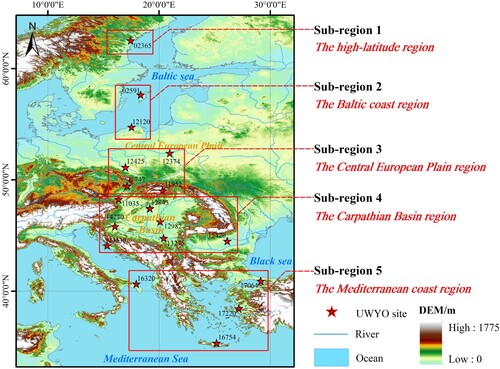
The UWYO profile is mainly provided by globally distributed radiosonde stations and generates the data set twice per day at 0 and 12 UTC (Universal Time Coordinated). The primary meteorological element fields include geopotential heights, pressures, air temperatures, relative humidity, and dew point temperatures. Since the AMSR2 detects the land surface at local times of 1:30 am and 1:30 pm, it is hard to acquire the UWYO profiles that are totally consistent with AMSR2 brightness temperature products in space and time. Thus, in order to guarantee that the time difference between the UWYO profiles and AMSR2 products is small and better acquire the cloudy-skies instantaneous LST in the following study, this study selected the UWYO profiles at 23 radiosonde stations (with longitudes ranging from 15°E to 30°E) at 12 UTC for the specific evaluation of reanalysis products. They are mainly distributed in Europe, Egypt, South Africa, and other places, with certain representativeness. The geographical locations and land-cover types of the selected 23 stations are displayed in Figure 1 in detail. Table 1 exhibits the detailed information of each station.

Figure 1. The geographic locations of the selected 23 radiosonde stations.

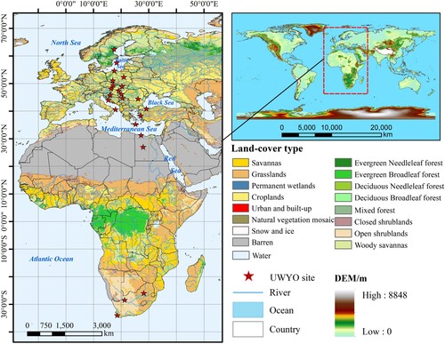
Table 1. A summary of the detailed information at 23 radiosonde stations.

Station ID	Station Name	Country	Longitude	Latitude	Elevation/m
02365	Sundsvall-Harnosand	Sweden	17.45°E	62.53°N	6
02591	Visby Aervlogiska Stn	Sweden	18.35°E	57.65°N	47
12120	Leba	Poland	17.53°E	54.75°N	6
12374	Legionowo	Poland	20.96°E	52.40°N	96
12425	Wroclaw	Poland	16.98°E	51.13°N	116
11747	Prostejov	Czech Republic	17.13°E	49.45°N	216
11952	Poprad-Ganovce	Slovakia	20.31°E	49.03°N	706
11035	Wien	Austria	16.36°E	48.25°N	200
12843	Budapest	Hungary	19.18°E	47.43°N	139
12982	Szeged	Hungary	20.10°E	46.25°N	83
14240	Zagreb	Croatia	16.03°E	45.82°N	246
13275	Beograd	Serbia	20.42°E	44.76°N	203
15420	Bucuresti lnmh-Banesa	Romania	26.13°E	44.50°N	91
14430	Zadar	Croatia	15.34°E	44.10°N	79
17064	Istanbul	Turkey	29.15°E	40.90°N	17
16320	Brindisi	Italy	17.95°E	40.65°N	10
17220	Izmir	Turkey	27.16°E	38.43°N	29
16754	LGIR Heraklion	Greece	25.18°E	35.53°N	39
62306	HEMM Mersa Matruh	Egypt	27.21°E	31.33°N	28
62423	Farafra	Egypt	27.96°E	27.05°N	92
68263	FAIR Pretoria (Irene)	South Africa	28.21°E	25.91°S	1523
68424	FAUP Upington	South Africa	21.26°E	28.41°S	839
68816	Cape Town Intnl. Arport	South Africa	18.60°E	33.96°S	42

In this study, a total of 2829 UWYO profiles were selected from 23 UWYO stations in January, April, July, and October of 2018, and the meteorological elements for each profile data point included the pressure, geopotential height, air temperature, and relative humidity values. The selected all UWYO profiles can be freely acquired from the website (http://weather.uwyo.edu/upperair/sounding.html).

2.2. Reanalysis atmospheric profile

Six reanalysis atmospheric profile products, including the ERA5, ERA-Interim, JRA-55, MERRA2, NCEP/FNL, and NCEP/GFS, were mainly applied in this study to implement the comparative evaluation. Table 2 displays the main characteristics of the six reanalysis profile products.

1. ERA5

Table 2. A summary of the main characteristics of six kinds of reanalysis profiles.

Reanalysis Data	Data Periods	Temporal Resolution	Spatial Resolution	Vertical Resolution	Website Link
ERA5	1979–present	1 hourly	0.25°×0.25°	37 pressure levels	https://cds.climate.copernicus.eu/cdsapp#!/search?type=dataset
ERA-Interim	1979–2019	6 hourly	0.75°×0.75°	37 pressure levels	http://apps.ecmwf.int/datasets/
JRA-55	1958–present	6 hourly	1.25°×1.25°	27 pressure levels	http://jra.kishou.go.jp/JRA-55/index_en.html
MERRA2	1980–present	3 hourly	0.25°×0.25°	42 pressure levels	https://disc.sci.gsfc.nasa.gov/
NCEP/FNL	1999–present	6 hourly	1.0°×1.0°	26 pressure levels	https://rda.ucar.edu/datasets/ds083.2/
NCEP/GFS	2007–present	6 hourly	0.5°×0.5°	31 pressure levels	https://nomads.ncdc.noaa.gov/data/gfsanl/n

ERA5 is the latest climate reanalysis product generated by the ECMWF for global climate change analyses and replaced the ERA-Interim reanalysis dataset after 31 August 2019 (Hersbach et al. 2020). This dataset is organized with a regular latitude-longitude grid at a 0.25°×0.25° resolution in GRIB or NetCDF format and possesses 37 pressure levels: 1000, 975, 950, 925, 900, 875, 850, 825, 800, 775, 750, 700, 650, 600, 550, 500, 450, 400, 350, 300, 250, 225, 200, 175, 150, 125, 100, 70, 50, 30, 20, 10, 7, 5, 3, 2, and 1 hPa. This data provides numerous meteorological elements, including the geopotential height, pressure, temperature, relative humidity, and specific humidity, from 1979 to the present, with an hourly temporal resolution.

• (2) ERA-Interim

ERA-Interim is another global atmospheric reanalysis dataset produced by the ECMWF that is currently available from 1 January 1979 to 31 August 2019 (Dee, Uppala, and Simmons 2011; Simmons et al. 2007). These reanalysis data were produced using the four-dimensional assimilation technique with a 12-hour analysis window in GRIB format. The nominal resolution of the dataset is 0.75°×0.75° at 37 pressure levels: 1000, 975, 950, 925, 900, 875, 850, 825, 800, 775, 750, 700, 650, 600, 550, 500, 450, 400, 350, 300, 250, 225, 200, 175, 150, 125, 100, 70, 50, 30, 20, 10, 7, 5, 3, 2, and 1 hPa. This dataset provides similar meteorological element information to that of the ERA5 profile product, including the geopotential height, pressure, air temperature, and relative humidity values recorded every six hours at 00, 06, 12, and 18 UTC.

• (3) JRA-55

The JRA-55 profile dataset is the second reanalysis project performed by the Japan Meteorological Agency (JMA) and is based on a more sophisticated data assimilation system (Kobayashi et al. 2015). Its data use period is 55 years, and regular radiosonde observation has been conducted worldwide since 1958. This dataset is produced with a spatial resolution of 1.25°×1.25° on 37 isobaric levels (1000, 975, 950, 925, 900, 875, 850, 825, 800, 775, 750, 700, 650, 600, 550, 500, 450, 400, 350, 300, 250, 225, 200, 175, 150, 125, 100, 70, 50, 30, 20, 10, 7, 5, 3, 2, and 1 hPa); but the specific humidity, relative humidity, and dew-point depression data are only available on the 27 levels from 1000 to 100 hPa. The JRA-55 data are organized in GRIB format and provided every six hours at 00, 06, 12, and 18 UTC.

• (4) MERRA2

MERRA-2 is a kind of reanalysis product from the National Aeronautics and Space Administration (NASA) containing data from 1980. It is generated via the Goddard Earth Observing System Model, Version 5 (GEOS-5) with the Atmospheric Data Assimilation System (ADAS), version 5.12.4 (Molod et al. 2014; Rienecker et al. 2011). Its spatial resolution is 0.625° longitude×0.5° latitude, and it contains data at 42 pressure levels: 1000, 975, 950, 925, 900, 875, 850, 825, 800, 775, 750, 725, 700, 650, 600, 550, 500, 450, 400, 350, 300, 250, 200, 150, 100, 70, 50, 40, 30, 20, 10, 7, 5, 4, 3, 2, 1, 0.7, 0.5, 0.4, 0.3, and 0.1 hPa. The meteorological elements provided in this product mainly include the geopotential height, pressure, air temperature, and relative humidity in NetCDF-4 format, reported every 6 h at 00, 06, 12, and 18 UTC.

• (5) NCEP/FNL

The NCEP/FNL profile is primarily produced by the Global Data Assimilation System (GDAS) by continually collecting and processing observational data from the Global Telecommunications System (GTS) and other sources for climate analyses (Zia ul Rehman et al. 2018). The dataset is organized on 1°×1° grids with the GRIB format. It is available on 26 mandatory levels from 1000 to 10 hPa (1000, 975, 950, 925, 900, 850, 800, 750, 700, 650, 600, 550, 500, 450, 400, 350, 300, 250, 200, 150, 100, 70, 50, 30, 20, and 10 hPa). The meteorological elements mainly include the geopotential height, air temperature, relative humidity, sea surface temperature, surface pressure, and surface soil values. This data can be obtained every six hours at 00, 06, 12, and 18 UTC from 1999 to the present.

• (6) NCEP/GFS

The NCEP/GFS is a global numerical weather prediction system containing a global computer model and variational analyses run by the United States (U.S.) National Weather Service (NWS) (Lima and Alcntara 2019). The generated profile dataset includes two kinds of grids of 0.5°×0.5° and 1°×1° and provides a total of 31 atmospheric levels at 1000, 975, 950, 925, 900, 850, 800, 750, 700, 650, 600, 550, 500, 450, 400, 350, 300, 250, 200, 150, 100, 70, 50, 30, 20, 10, 7, 5, 3, 2, and 1 hPa. The meteorological parameter fields of this dataset include the geopotential height, relative humidity, air temperature, ozone, soil moisture, and precipitation. The dataset is reported four times per day at 00, 06, 12, and 18 UTC from 1 January 2007 to 15 May 2020. In this study, the NCEP/GFS profile with a spatial resolution of 0.5°×0.5° in the GRIB format was used.

2.3. AMSR2 brightness temperature product

AMSR2 is a passive microwave radiometer designed by the Japan Aerospace Exploration Agency (JAXA) on 18 May 2012 and is installed in the Global Change Observation Mission-Water (GCOM-W) satellite. It contains seven channels at 6.925, 7.3, 10.65, 18.7, 23.8, 36.5, and 89.0 GHz, with horizontal and vertical polarization at each channel. The instantaneous field of view varies from 3 km×5 km at 89.0 GHz to 35 km×62 km at 6.925 GHz, and the Earth incidence angle is 55°. It probes the Earth’s surface twice per day, and the transiting times are approximately 1:30 am (descending orbit) and 1:30 pm (ascending orbit) local time at the equator (Imaoka et al. 2010). At present, for the sake of the extensive application of the data recorded by this instrument for hydrological balance research, AMSR2 has produced three kinds of brightness temperature products, including Level 1B, Level 1R, and Level 3. Among them, the Level-3 brightness temperature has a resolution of 0.1°×0.1° for all channels and achieves good accuracy (Maeda, Taniguchi, and Imaoka 2016). As a result, this study mainly used the AMSR2 Level-3 brightness temperature product to retrieve LSTs under cloud-covered skies. These products can be freely acquired from the G-Portal tool (ftp.gportal.jaxa.jp).

3. Methodology

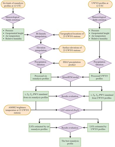
Figure 2 presents a flowchart used for clearly describing the evaluation process of the performances of six reanalysis profile products in the atmospheric correction of passive microwave data when estimating land surface temperature under cloudy-sky conditions. This flowchart mainly includes atmospheric parameter estimation with the MonoRTM, LST retrieval under cloudy skies with Weng’s algorithm, and evaluations of atmospheric parameter and LST. The specific methods are described as follows.

Figure 2. Flowchart of evaluation of six reanalysis profile products.

3.1. Atmospheric parameter estimation with MonoRTM

Removing atmospheric effects in the microwave region is an essential process when applying the AMSR2 brightness temperature data to derive the LSTs under cloudy-sky conditions. In combination with the acquired UWTO profile and six reanalysis profile products, the Monochromatic Radiative Transfer Model (MonoRTM 5.4) developed by Atmospheric & Environmental Research (AER) (Clough et al. 2005) was applied in this paper to estimate the transmittance (τ), atmospheric upward radiance (T_u), atmospheric downward radiance (T_d), and precipitable water vapor (PWV) values at seven frequencies of the AMSR2 brightness temperature.

According to the atmospheric radiation transmission theory in the microwave region, τ can be expressed as follows (Ulaby, Moore, and Fung 1986): (1) $\begin{array}{rl}& \tau (f,\theta )=e^{-\mathrm{\Gamma }(f,\theta )/\cos \theta }\\ & \mathrm{\Gamma }(f,\theta )=\mathrm{s}\mathrm{e}\mathrm{c}\theta \left[{\int }_0^{\mathrm{\infty }}\kappa o2\right(f,z)dz+{\int }_0^{\mathrm{\infty }}\kappa vap(f,z)dz+{\int }_0^{\mathrm{\infty }}\kappa liq(f,z\left)dz\right]\end{array}$(1) where τ(f, θ) is the atmospheric transmittance at frequency f and zenith angle θ; Γ(f, θ) is the atmospheric optical thickness at frequency f and zenith angle θ; κ(f, z) is the atmospheric attenuation coefficient at frequency f and height z; and κ_o2(f, z), κ_vap(f, z), κ_liq(f, z) are the atmospheric attenuation coefficients of O₂, WV, and CLW at frequency f and height z, respectively.

The T_u and T_d values derived from the atmosphere in the microwave region can be treated as a function of the kinetic temperature (T) and τ under any weather conditions, respectively, and can be expressed as follows: (2) $T\mathrm{u}(f,\theta )=\sec \theta {\int }_0^{H}T\left(z\right)\kappa (f,z)\exp (-\mathrm{\Gamma }(f,z,H)\cdot \sec \theta )dz$(2) (3) $T\mathrm{d}(f,\theta )=\sec \theta {\int }_0^{\mathrm{\infty }}T\left(z\right)\kappa (f,z)\exp (-\mathrm{\Gamma }(f,0,z)\cdot \sec \theta )dz$(3) where T_u(f, θ) and T_d(f, θ) are the upward radiation and downward radiation, respectively, at frequency f and zenith angle θ (K); H is the atmospheric height (km); T(z) and κ(f, z) are the mean temperatures of the atmospheric components and atmospheric attenuation coefficient at frequency f and height z (K), respectively; and exp(-Γ(f, 0, z)·secθ) refers to the atmospheric transmittance at frequency f, height z, and zenith angle θ.

The PWV is calculated from the obtained pressure, air temperature, and specific humidity profiles: (4) $PWV={\displaystyle \frac{1}{{\rho }_{w}g}{\int }_{p_s}^{0}q\left(P\right)dP}$(4) where ρ_w is the liquid water density (1000 kg/m³); g is the gravitational acceleration at the pressure level height (9.8 m/s²); P_s is the pressure (hPa); q(P) is the mixing ratio (g/kg) of atmospheric water vapor.

Prior to estimating the atmospheric parameters, since there are obvious differences between the meteorological element fields of the UWYO profile and those of the other six reanalysis profiles, we merely selected the same meteorological elements from the UWYO profile and six kinds of reanalysis profiles, i.e. the geopotential height, pressure, air temperature, and relative humidity. Usually, these four meteorological elements can represent the basic conditions of the atmosphere. Then, in order to obtain atmospheric parameters station-by-station in the reanalysis products, the selected reanalysis profile data were interpolated in time, space, and elevation, with the processing method proposed by Barsi, Barker, and Schott (2003) and Yang et al. (2020), as follows.

1. The six reanalysis profile products at the UWYO observation time (i.e. 12 UTC) were respectively extracted from the corresponding reanalysis dataset.

2. The six reanalysis profiles at 12 UTC were further bi-linearly interpolated in space with the geographic latitude and longitude of four grid net points closest to 23 radiosonde stations since the bilinear interpolation has good accuracy and efficiency.

3. The reanalysis profiles of 23 radiosonde stations at 12 UTC were all adjusted to the actual elevation from the land surface to the top layer of the atmosphere using the surface elevation of each UWYO station.

Furthermore, because the microwave signal penetrating a rainy region will undergo a very significant attenuation effect (Ulaby, Moore, and Fung 1986), in order to further reduce the errors of atmospheric parameters estimated at heavy precipitation conditions, the UWYO profile and six reanalysis profiles obtained under heavy precipitation were filtered using the ERA5 precipitation product. This screening process will be helpful for subsequent comparative analysis of six reanalysis profile products.

With the above-described processing steps, based on the observation angle of the AMSR2 sensor (55°), the processed UWYO profile and six reanalysis profiles were all input into the MonoRTM to calculate station-by-station four kinds of atmospheric parameters (τ, T_d, T_u, and PWV) under non-precipitation conditions.

3.2. LST retrieval under cloudy skies

In this study, the physics-based LST retrieval algorithm proposed by Weng and Grody (1998) was applied to the AMSR2 brightness temperature products to derive the LSTs under cloudy skies. This algorithm assumes that the LSEs at two adjacent frequencies (i.e. 18.7 and 23.8 GHz) are nearly identical and that the transmittance of clouds (as well as oxygen) at these two frequencies is also nearly identical. The main difference between the atmospheric emissions at these two frequencies is mainly caused by the differential absorption effects of atmospheric water vapor (Duan, Li, and Leng 2017). This algorithm possesses a very clear physical meaning but cannot be employed for heavy precipitation weathers and deep snow-covered surfaces over a global scale since these conditions can affect low-frequency measurements via generating scattering effects. In previous works of Weng and Grody (1998), it was stated that the LST retrieval algorithm used performed well for the non-scattering conditions, with large biases occurring under the scattering conditions.

For non-scattering, plane-parallel atmosphere conditions, the radiation brightness temperature received by the PMW radiometer for non-black body boundaries can be expressed as three main processes from the top of atmospheric (TOA) to the land surface: (i) radiation emitted from the land surface and attenuated by the atmosphere; (ii) upward radiation emitted by the atmosphere; and (iii) downward radiation from the atmosphere and cosmic background reflected by the land surface and attenuated by the atmosphere (Weng and Grody 1998). It is assumed that the T_u is equal to the T_d in the microwave region, the TOA brightness temperature can be further expressed as follows when the atmosphere is considered isothermal (T_m): (5) $T\mathrm{b}=T\mathrm{s}[1-(1-ϵ\left)e^{-2\tau }\right]-\mathrm{\Delta }T(1-e^{-\tau })[1+(1-ϵ\left)e^{-\tau }\right]$(5) where T_b is the TOA brightness temperature; T_s is the land surface temperature (K); ϵ is the land surface emissivity; τ is the atmospheric transmittance; and ΔT = T_s - T_m is the difference between the LST and the isothermal atmospheric temperature.

From the radiative transfer simulation, the second term on the right-hand side of Eq. (5) is found to be insensitive to the LSE and can be parameterized as a function of PWV for high-emissivity surfaces (ϵ > 0.9) (Weng and Grody 1998). This relationship results in the following equation: (6) $T\mathrm{b}=T\mathrm{s}[1-(1-ϵ\left)e^{-2\tau }\right]-\gamma PWV$(6) where γ is the frequency-dependent regression coefficient.

Meanwhile, previous studies have found that the LSEs at two adjacent frequencies are nearly the same and that the atmospheric emission is significantly different at these two frequencies (Matzlar 1994); thus, a relatively stable relationship can be obtained at 18.7 and 23.8 GHz with the vertical polarization as follows: (7) ${\displaystyle \frac{T\mathrm{s}-T\mathrm{b},18.7\mathrm{V}-\gamma 18.7\cdot PWV}{T\mathrm{s}-T\mathrm{b},23.8\mathrm{V}-\gamma 23.8\cdot PWV}={\left({\displaystyle \frac{{\mathrm{e}}^{-\tau 18.7}}{{\mathrm{e}}^{-\tau 23.8}}}\right)}^2}$(7) where T_b,18.7V and T_b,23.8V are the radiation brightness temperatures observed by the PMW radiometer at frequencies of 18.7 and 23.8 GHz with vertical polarization, respectively; τ_18.7 and τ_23.8 are the transmittances at frequencies of 18.7 and 23.8 GHz, respectively; and γ_18.7 and γ_23.8 are two constants that depend on the frequency. Here, γ_18.7 = 0.047 and γ_23.8 = 0.136.

Since the atmospheric parameters τ_18.7, τ_23.8 and PWV in Eq. (7) can be simulated with the atmospheric profiles in combination with the MonoRTM, the LSTs under cloudy-sky conditions can be acquired in the end as follows: (8) $Ts={\displaystyle \frac{(T\mathrm{b}18.7v\tau {23.8}^2-Tb23.8v\tau {18.7}^2)+(\gamma 18.7PWV\cdot \tau {23.8}^2-\gamma 23.8PWV\cdot \tau 18.7^2)}{\tau {23.8}^2-\tau {18.7}^2}}$(8)

From Eq. (8), we can notice that the LST under cloudy skies can be acquired by using the AMSR2 brightness temperatures obtained at frequencies of 18.7 and 23.8 GHz and by eliminating the LSEs at these two frequencies. However, it is more important to accurately obtain three atmospheric parameters when the cloudy-sky LST is estimated. Thus, it is necessary to evaluate the applicability of the τ and PWV derived from various reanalysis profile products and select the best reanalysis profiles for accurately retrieving cloudy-sky LSTs.

3.3 Assessment indicator

The estimated atmospheric parameters (τ, T_u, T_d, and PWV) derived from the UWYO profile were regarded as actual atmospheric profiles to evaluate the other six reanalysis profile products. Moreover, the corresponding τ and PWV were imported into the LST retrieval algorithm proposed by Weng and Grody (1998) to analyze the applicability of various reanalysis atmospheric profiles in retrieving LSTs under cloudy skies. In this study, the RMSE, relative RMSE (RRMSE), and coefficient of determination (R²) were used as three indicators to quantify the performance of the six reanalysis profiles. These three indicators are frequently employed to evaluate the accuracy of data. In general, the closer the RMSE and RRMSE values are to 0, the closer the reanalysis profile is to the actual UWYO profile; the closer R² is to 1, the better the reanalysis profile performs. Mathematically, for each reanalysis profile, RMSE, RRMSE, and R² are defined as follows: (9) $RMSE=[n^{-1}\sum _{i=1}^n{(\overline{par}-par)}^2{]}^{1/2}$(9) (10) $RRMSE={\displaystyle \frac{{\left[n^{-1}{\sum }_{i=1}^n{(\overline{par}-par)}^2\right]}^{1/2}}{{\displaystyle \frac{1}{n}{\sum }_{i=1}^{n}par}}}$(10) (11) $R^2=1-{\displaystyle \frac{{\sum }_{i=1}^n{(\overline{par}-\overline{pa{r}_{\mathrm{m}\mathrm{e}\mathrm{a}\mathrm{n}}})}^2}{{\sum }_{i=1}^n{(par-pa{r}_{\mathrm{m}\mathrm{e}\mathrm{a}\mathrm{n}})}^2}}$(11) where RMSE is the root-mean-square error; n is the number of atmospheric profiles; $\overline{par}$ represents the simulated atmospheric parameters (i.e. τ, T_u, T_d, and PWV) derived from the six reanalysis profiles; par represents the actual atmospheric parameters (i.e. τ, T_u, T_d, and PWV) derived from the UWYO profile; RRMSE is the relative RMSE; R² is the coefficient of determination; $\overline{pa{r}_{\mathrm{m}\mathrm{e}\mathrm{a}\mathrm{n}}}$ is the average of the simulated atmospheric parameters derived from the six reanalysis profiles; and par_mean is the average of the actual atmospheric parameters derived from the UWYO profile.

3.4. Sensitivity analysis of LST retrieval to the atmospheric parameters

The uncertainty of atmospheric parameters ultimately determines the accuracy of LST retrievals. Assuming that the LST retrieval algorithm proposed by Weng and Grody (1998) can characterize the true LST values and that the AMSR2 brightness temperatures do not contain noise equivalent to the temperature differences, the sensitivities of LST retrievals to different atmospheric parameters can be evaluated as a combination of the uncertainties of τ₁₈, τ_23, and PWV and can be expressed as follows: (12) ${\mathrm{\Delta }T}_{\mathrm{s}}^{\mathrm{t}\mathrm{o}\mathrm{t}\mathrm{a}\mathrm{l}}=\sqrt{{\left({\mathrm{\Delta }T}_{\mathrm{s}}^{\tau 18}\right)}^2+{\left({\mathrm{\Delta }T}_{\mathrm{s}}^{\tau 23}\right)}^2+{\left({\mathrm{\Delta }T}_{\mathrm{s}}^{\mathrm{P}\mathrm{W}\mathrm{V}}\right)}^2}$(12) with (13) ${\mathrm{\Delta }T}_{\mathrm{s}}^{\tau 18}={\displaystyle \frac{\delta T\mathrm{s}}{\delta T\tau 18}\delta T\tau 18}$(13) (14) ${\mathrm{\Delta }T}_{\mathrm{s}}^{\tau 23}={\displaystyle \frac{\delta T\mathrm{s}}{\delta T\tau 23}\delta T\tau 23}$(14) (15) ${\mathrm{\Delta }T}_{\mathrm{s}}^{\mathrm{P}\mathrm{W}\mathrm{V}}={\displaystyle \frac{\delta T\mathrm{s}}{\delta T\mathrm{P}\mathrm{W}\mathrm{V}}\delta T\mathrm{P}\mathrm{W}\mathrm{V}}$(15) where $\mathrm{\Delta }{T}_{\mathrm{s}}^{\mathrm{t}\mathrm{o}\mathrm{t}\mathrm{a}\mathrm{l}}$ is the total LST uncertainty derived from three atmospheric parameters in the LST retrieval process; $\mathrm{\Delta }{T}_{\mathrm{s}}^{\tau 18}$ and $\mathrm{\Delta }{T}_{\mathrm{s}}^{\tau 23}$ are the LST uncertainties associated with τ₁₈ and τ₂₃, respectively; and $\mathrm{\Delta }{T}_{\mathrm{s}}^{\mathrm{P}\mathrm{W}\mathrm{V}}$ is the LST uncertainty associated with PWV. Regarding the six reanalysis profile products, δT_τ18, δT_τ23 and δT_PWV can be acquired after τ₁₈, τ₂₃ and PWV are evaluated, respectively. With Eq. (11), the accuracies of the six reanalysis profiles can be further compared by discussing the sensitivities of various atmospheric parameters to the LST retrievals.

4. Results

4.1. Assessment of atmospheric parameters derived from reanalysis profiles

Since the atmospheric molecules have different responses to the electromagnetic wave, the values of T_d, T_u, and τ vary by microwave channels. In order to reveal the change characteristics of T_d, T_u, and τ at various frequencies, six reanalysis profile products at 23 UWYO stations were input into the MonoRTM 5.4 to estimate T_d, T_u, and τ and then calculated the average values of these three atmospheric parameters at seven frequencies in the AMSR2.

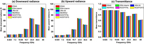
Figure 3(a)-(c) clearly presents the mean values of T_d, T_u, and τ simulated from six reanalysis profiles at seven frequencies in the AMSR2 brightness temperature products, respectively. For all reanalysis profiles, the transmittances for low frequencies (<18.7 GHz) were almost above 0.97, and the produced brightness temperatures were all less than 5.50 K at these frequencies. This indicates that the brightness temperature changes at lower frequencies derived from various atmospheric compositions can be ignored under cloudy-skies conditions to some extent. However, at frequencies of 23.8, 36.5, and 89 GHz, the total transmittances caused by atmospheric compositions such as WV and O₂ were under 0.86, producing some larger atmospheric radiation information (generally greater than 31 K). This shows that the atmospheric correction of brightness temperatures obtained under cloudy conditions is a key step to improving the retrieval accuracies of surface biophysical parameters using the PMW remote sensing technology. On the other hand, we found from Figure 3 that the atmospheric radiance values (T_d and T_u) calculated from the JRA-55, NCEP/FNL, and NCEP/GFS profiles were generally underestimated and produced higher atmospheric transmittances than the other reanalysis profile products, especially at high frequencies (>18.7 GHz). This result is because the atmospheric absorption and radiation in higher-frequency regions depend strongly on the vertical distributions of atmospheric humidity profiles and are greatly affected by WV and CLW. Since the JRA-55, NCEP/FNL, and NCEP/GFS profile products all have lower vertical resolutions (i.e. their pressure levels are lower), they can detect less atmospheric humidity information, thus generating lower atmospheric radiance values and higher transmittance values.

Figure 3. Mean values of three atmospheric parameters simulated from the six reanalysis profiles at AMSR2 frequencies. (a) mean values of T_d; (b) mean values of T_u; (c) mean values of τ.

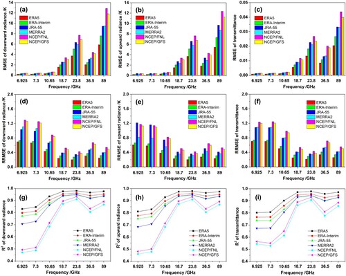
Taking the atmospheric parameters simulated from the UWYO profile as the actual values, Figure 4(a)-(f) compares the RMSE, RRMSE, and R² values of three parameters simulated from the other six reanalysis profiles at seven frequencies in the AMSR2 brightness temperatures. It is quite evident that, except for the frequency of 23.8 GHz, in which the atmospheric radiation is mainly impacted by water vapor absorption, the RMSE changes in all reanalysis profiles were closely associated with the microwave frequencies. As the frequency rises, accordingly, the RMSEs gradually increase. This was relatively consistent with the changes observed in three atmospheric parameter values at different frequencies, indicating that the higher the microwave frequency is, the larger the generated errors derived from various reanalysis profiles are. Nevertheless, the RRMSE and R² values between the UWYO profile and the other six reanalysis profiles performed better at 18.7 and 23.8 GHz and performed poorly at frequencies of 6.932 and 7.3 GHz. This finding indicates that any reanalysis profile can be recommended to better estimate atmospheric parameters at frequencies of 18.7 and 23.8 GHz compared to other frequencies. Furthermore, for all AMSR2 frequencies, the ERA5 profile generated the best accuracies of atmospheric parameter estimations, with average RMSE values of 2.01, 1.89 K, and 0.007 for T_d, T_u, and τ, respectively. The ERA-Interim also exhibited a better performance in assessing these three parameters at all microwave frequencies. The JRA-55 profile possessed similar accuracy as those of the MERRA2 profile when the frequency was less than 18.7 GHz and obtained better results than the NCEP/GFS and NCEP/FNL profiles but performed poorer than the MERRA2 profile when the frequency was greater than 18.7 GHz. However, since the NCEP/FNL had the lowest vertical resolution, its accuracy when predicting atmospheric parameters was the lowest among all reanalysis profiles, with mean RMSEs of approximately 4.28, 4.15 K, and 0.014 for T_d, T_u, and τ, respectively.

Figure 4. The RMSE, RRMSE, and R² changes of T_d, T_u, and τ simulated from the six reanalysis products and the UWYO profile at seven frequencies. (a) RMSE changes of T_d; (b) RMSE changes of T_u; (c) RMSE changes of τ; (d) RRMSE changes of T_d; (e) RRMSE changes of T_u; (f) RRMSE changes of τ; (g) R² changes of T_d; (h) R² changes of T_u; (i) R² changes of τ.

Overall, the accuracies of three atmospheric parameters estimated from the ERA5 profile were better than those of the atmospheric parameters obtained from the remaining reanalysis profile products, and the accuracies of the ERA-Interim, MERRA2, JRA-55, NCEP/GFS, and NCEP/FNL profiles gradually decreased. To be specific, these results could be attributed to some extent to the spatial resolution and vertical resolution of the reanalysis atmospheric profiles.

4.2. Impacts of various reanalysis profiles on LST retrievals

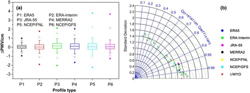
Since PMW-based LST retrievals require PWV as an input, it is also necessary to analyze the differences among PWV values estimated using different reanalysis products before discussing the impacts of various reanalysis profiles on LST retrievals. Figure 5(a) first displays a boxplot of the differences among the PWVs that were calculated from the UWYO profile and the other six reanalysis profiles. From Figure 5(a), we observed that the ERA5 profile obtained the best results than the other reanalysis profiles in estimating PWV, with the mean ΔPWV of 0.054 cm, the minimum ΔPWV of −0.952 cm, and the maximum ΔPWV of 0.996 cm, respectively. The ERA-Interim profile also presented well and had smaller outliers than the rest of the reanalysis profile products but had large fluctuation compared with the ERA5 profile (ΔPWV varied from −1.907 cm to 1.777 cm). Concerning the MERRA2, JRA-55, NCEP/GFS, and NCEP/FNL profiles, their ΔPWVs showed a fluctuating state and generated some larger outliers. This finding suggests that their accuracies gradually decreased. Additionally, Figure 5(b) exhibits a Taylor diagram of the PWVs simulated from the UWYO observations and the other six reanalysis profile products. In this section, standard deviation (STD), root mean squared deviation (RMSD), and correlation coefficient (R) were used as three assessment criteria to characterize the performances of the PWVs simulated from the other six reanalysis products. In Figure 5(b), the ERA5 profile generated the lowest RMSD of 0.282 cm and obtained the highest R of 0.982 compared with the other reanalysis profile products, and its STD of 1.48 cm was the closest to the STD of the UWYO profile (1.53 cm). The ERA-Interim profile displayed a similar performance to the ERA5 profile, whereas its RMSD was higher (0.415 cm) than that of the ERA5 profile (0.282 cm). Regarding the MERRA2, JRA-55, NCEP/GFS, and NCEP/FNL profiles, their PWV RMSDs ranged from 0.50 cm to 0.62 cm, their PWV STDs ranged from 1.38 cm to 1.50 cm, and their PWV Rs were all greater than 0.912. However, it is worth noting that the NCEP/GFS profile obtained the smallest STD at 1.38 cm, followed by the NCEP/FNL profile at 1.40 cm. These findings were inconsistent with the actual PWV fluctuation simulated by the UWYO profile, indicating that the selected NCEP/GFS and NCEP/FNL profiles could not reveal the actual status of PWV changes in different months. The leading cause of this result is that these two kinds of reanalysis profiles possess poor atmospheric vertical distribution patterns.

Figure 5. (a) Boxplot of the differences between the PWVs simulated from the UWYO profile and the other six reanalysis profiles; (b) Taylor diagrams of PWVs simulated from the six reanalysis profile products and UWYO observations.

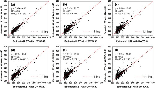
According to the aforementioned results, we can conclude that the ERA5 profile obtained the highest accuracy in estimating the actual atmospheric parameters compared with the other five reanalysis profiles overall. However, to further evaluate the accuracies of the reanalysis profiles in assisting the atmospheric correction of LSTs under cloudy skies, the LSTs retrieved with the UWYO profile were designated as the reference and contrasted with those obtained using the other six reanalysis profiles. Figure 6(a)-(f) displays scatterplots of the LSTs estimated from the UWYO profile versus the LSTs estimated from the other six reanalysis profiles. Before analysis, the LST values above 273.15 K were retained for revealing the LST change under the conditions of no snow cover due to the scattering effect of snow. Compared with the referenced LST, the R² values of the six reanalysis profile products were all higher than 0.7, whereas the RMSEs of the LSTs retrieved with different reanalysis profile products were obviously different and varied from 3.15 K to 6.12 K. Among them, the ERA5 profile presented the highest R² value with a value of 0.92 and the smallest RMSE with a value of 3.15 K, and its scatter point distribution was the closest to the 1:1 line. Moreover, good performance with an RMSE of 4.79 K was found for the ERA-Interim profile, followed by the NCEP/GFS profile with an RMSE of 5.22 K. In addition, similar performances were achieved using the MERRA2 and JRA-55, and the overall LST RMSEs calculated from these two profiles were 5.44 and 5.74 K, respectively. Not surprisingly, the worst LST retrieval result was observed by the NCEP/FNL profile, with R² and RMSE values of approximately 0.72 and 6.12 K, respectively. The specific reason for the poor accuracy performance of the NCEP/FNL profile can be attributed to the lower spatial resolution with 1°×1° and the poorer vertical resolution with 26 levels.

Figure 6. Scatterplots of LSTs derived from the UWYO profile versus LSTs derived from the other six reanalysis profiles. (a) ERA5; (b) ERA-Interim; (c) JRA-55; (d) MERRA2; (e) NCEP/FNL; (f) NCEP/GFS.

Since the parameters of the LST retrieval equation are the same for all reanalysis profiles except the atmospheric parameters, it can be concluded that the discrepancies between the LSTs derived from the six profiles were mainly caused by differences among the six atmospheric reanalysis profiles. From the above results, it can be seen that the ERA5 profile is relatively suitable for atmospheric corrections of microwave channel data and can obtain relatively accurate LSTs under cloudy conditions.

4.3. Sensitive analyses of LST retrievals to various atmospheric parameters

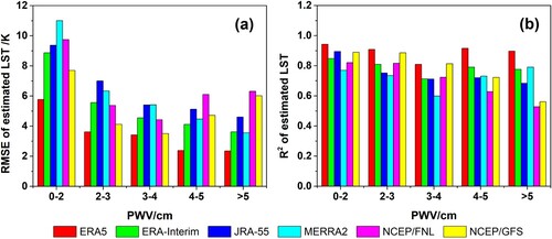
To further illustrate the accuracies of the six reanalysis profiles when atmospherically correcting LSTs obtained under cloud-covered conditions, the LST retrieval results were divided into five groups according to the PWV values, 0∼2 cm, 2∼3 cm, 3∼4 cm, 4∼5 cm, and > 5 cm, for an in-detail assessment. Figure 7(a)-(b) shows histograms of the LST RMSEs and R² values at various PWV levels. It is obvious from Figure 7 that the ERA5 profile showed the lowest RMSEs and the highest R² values at all PWV levels, indicating that the ERA5 profile can be better recommended for the atmospheric correction of LSTs obtained for different water vapor distribution conditions. The ERA-Interim, MERRA2, and JRA-55 profiles presented higher RMSE values than the other reanalysis profiles when PWV was less than 4 cm, whereas their RMSEs were less than that of the NCEP/FNL profile when PWV was greater than 4 cm. The NCEP/FNL and NCEP/GFS profiles showed lower RMSE values and higher R² values than MERRA2, JRA-55, and ERA-Interim products when PWV was less than 4 cm, whereas the growth rate of the RMSE was relatively obvious when PWV was greater than 4 cm. There are two possible reasons explaining this finding. First, the uncertainties of τ and PWV in the NCEP/FNL and NCEP/GFS profiles are relatively high, as perceived from Figures 4 and 5. Second, the LST retrieval algorithm derived by Weng and Grody (1998) is very sensitive to the atmospheric water vapor content, as demonstrated by previous studies (Huang et al. 2019). From the overall change trend of the LST RMSEs at various PWV levels, we found that, in addition to the NCEP/FNL and NCEP/GFS profiles, as the water vapor content increases, the accuracy of Weng’s algorithm improves. The RMSE values at high water vapor content levels are smaller than those at low water vapor content conditions. This result clearly indicates that Weng’s algorithm is more applicable under high-PWV conditions.

Figure 7. The accuracy assessment of estimated LSTs at various PWV levels. (a) RMSE; (b) R².

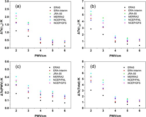
After comparing the accuracies of the six reanalysis profiles in atmospherically correcting the LSTs at five PWV levels, we further discussed the sensibilities of τ_18.7, τ_23.8, and PWV to LST retrievals results in Figure 8. As displayed in Figure 8(a)-(c), the LST uncertainties that are closely associated with errors in τ_18.7, τ_23.8, and PWV vary among the various reanalysis profiles when PWVs vary from 2 cm to 6 cm. Because the ERA5 and ERA-Interim profiles possessed the best accuracies when estimating atmospheric parameters, the LSTs retrieved using these profiles were impacted little by the changes in τ_18.7, τ_23.8, and PWV at all PWV levels. However, the LSTs estimated by the NCEP/FNL, NCEP/GFS, and JRA-55 profile products suffered greatly from the variations in these three atmospheric parameters. Especially for the total LST uncertainties, according to Figure 8(d), we found that the NCEP/FNL, NCEP/GFS, and JRA-55 profiles resulted in larger uncertainties than the ERA5 profile, and their uncertainties all were greater than 5 K when PWV is equal to 2 cm. In addition, for each reanalysis profile, we perceived that the sensibilities of τ_18.7, τ_23.8, and PWV to the LSTs exhibited similar performances. The LST uncertainties arising due to the uncertainties in PWV presented the smallest effects on the retrieved LSTs, with uncertainties ranging from 0.06 K to 0.41 K, whereas the LST uncertainties arising due to the uncertainties in τ_18.7 presented significant effects on the retrieved LSTs, with uncertainties ranging from 0.12 K to 2.24 K. More importantly, τ_23.8 had a quite large effect on the uncertainty of the estimated LSTs for all reanalysis profiles, and the LST uncertainties varied from 0.41 K to 5.53 K. This finding indicated that the pivotal atmospheric parameter controlling the accuracies of LST retrievals was τ_23.8, regardless of whether the conditions comprised clear skies or cloudy skies. For instance, an introduced RMSE of 0.013 in τ_23.8 for the ERA5 reanalysis product can result in an LST error as high as 2.87 K when PWV is 2 cm. The main reason for this error is that the 23.8 GHz frequency is located near the water vapor absorption zone and has a relatively low τ value, which can produce significant extra radiances in different weather conditions and regions.

Figure 8. The sensibilities of τ_18.7, τ_23.8, and PWV derived from the other six reanalysis profiles to the LST retrieval under five kinds of atmospheric conditions.

Obviously, effectively estimating atmospheric parameters with a good degree of precision is very important for retrieving LSTs under cloudy skies. The effects of τ_18.7 and τ_23.8 on electromagnetic waves are very evident in the AMER2-based LST retrievals, in particular, τ_23.8 significantly affects LST estimations. However, overall, the ERA5 profile is the most suitable for the atmospheric correction of LSTs obtained in cloud-covered regions at different water vapor contents. This is mainly attributed to this product generated the highest accuracy when estimating atmospheric parameters compared with the other reanalysis profiles.

5. Discussion

5.1. Spatiotemporal applicability of various reanalysis profile products

The three atmospheric parameters simulated from the six reanalysis profile products are significantly variable both spatially and temporally. Thus, it is also necessary to further compare the accuracies of these atmospheric profiles at various spatiotemporal scales. In consideration of the distribution characteristics of 23 UWYO stations, we first divided the six reanalysis profile products in Europe into five groups based on the latitude, topography, and land-sea distribution: the high-latitude region (sub-region 1), the Baltic coast region (sub-region 2), the Central European Plain region (sub-region 3), the Carpathian Basin region (sub-region 4), and the Mediterranean coast region (sub-region 5), then discussed the differences among the six reanalysis profiles in these sub-regions. The detailed geographic locations of five sub-regions are displayed in Figure 9.

Figure 9. Geographic distribution map of five sub-regions.

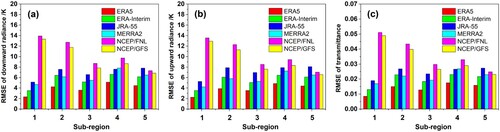
Since the frequency of 23.8 GHz has a particular response to water vapor variations, Figure 10 discusses the various impacts of the geographical distribution of the UWYO stations on the performance of the six reanalysis products at this frequency. Overall, regardless of which sub-regions were investigated, the ERA5 profile always performed best, followed by the ERA-Interim, MERRA2, JRA-55, NCEP/GFS, and NCEP/FNL profile products. Specifically, in addition to the NCEP/FNL and NCEP/FNL profiles, the other reanalysis profile products all had the best accuracies in sub-region 1, followed by sub-region 3, sub-region 5, sub-region 2, and sub-region 4, as a whole. For sub-region 4, since the basin has the effect of gathering water vapor, the performances of four profiles were strongly affected by water vapor changes, with larger RMSEs. Meanwhile, due to the evaporation effect of water vapor in the Baltic Sea and the Mediterranean Sea, the four reanalysis profiles also presented poor accuracies in sub-regions 2 and 5. In contrast, the four reanalysis profiles performed better in the inland regions, such as in sub-region 3. The RMSEs of τ at sub-region 3 varied from 0.01277 for the ERA5 to 0.02341 for the JRA-55. The above results indicated that the performances of reanalysis profiles suffered from the terrain and sea-land distribution characteristic. However, from the performances of the NCEP/FNL and NCEP/GFS profiles, we noted that the performances of profiles not only suffered from the sea-land distribution but were also affected by latitude. At sub-regions 1 and 2, the NCEP/FNL and NCEP/GFS profiles exhibited poor accuracies, with RMSEs greater than 0.048 for the NCEP/FNL profile and 0.052 for the NCEP/GFS profile in sub-region 1 in terms of τ_23.8. The main cause of this result is that the thickness of the troposphere is closely associated with latitude. In some high-latitude regions, such as Sundsvall-Harnosand, the relatively poor vertical resolutions of the NCEP/FNL and NCEP/GFS profiles impacted the accuracies of the atmospheric parameters to a great extent.

Figure 10. Histograms of RMSEs for three atmospheric parameters simulated from the six reanalysis profiles at various sub-regions of Europe. (a) RMSE of T_d; (b) RMSE of T_u; (c) RMSE of τ.

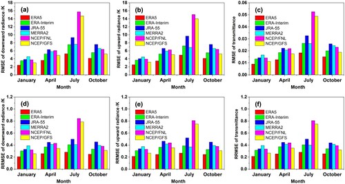
By dividing the stimulated atmospheric parameters into four groups based on month, Figure 11 further compares the RMSE and RRMSE differences among the six reanalysis profiles at four months at 23.8 GHz. It is pronounced that the RMSEs and RRMSEs of the three atmospheric parameters for all reanalysis profiles were higher in July than those in the other months due to the higher water vapor fluctuations. However, in January, the RMSEs and RRMSEs of the three atmospheric parameters derived from all reanalysis profiles performed the best compared with other months. This result again demonstrated that the performances of the reanalysis profiles are closely associated with the water vapor distribution. As such, choosing an accurate atmospheric profile to simulate these three atmospheric parameters in regions and periods with strong water vapor content is crucial. Regarding the performances of various reanalysis profiles, the ERA5 profile still obtained the best accuracy in revealing the actual atmospheric conditions, and RMSEs (RRMSEs) varied in the range from 0.0089 (0.212) in January to 0.0184 (0.281) in July for τ_23.8, followed by the ERA-Interim, which had a similar performance. However, the NCEP/FNL and NCEP/GFS profiles in July were greatly affected by the water vapor and performed poorly, and they performed better in the other months than the JRA-55 and MERRA2 profiles.

Figure 11. Histograms of RMSEs and RRMSEs for three atmospheric parameters simulated from the six reanalysis profiles at various months. (a) RMSE of T_d; (b) RMSE of T_u; (c) RMSE of τ; (d) RRMSE of T_d; (e) RRMSE of T_u; (f) RRMSE of τ.

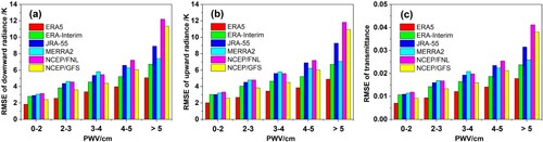
In addition, since the PWV is a crucial parameter impacting the simulation accuracy of LST estimations using different reanalysis profiles, Figure 12 also analyzes the RMSE differences among the six reanalysis profiles at five PWV levels for the 23.8 GHz. Similar to the results described above, the ERA5 and ERA-Interim profiles had small RMSEs for the three atmospheric parameters with various water vapor distribution levels. The NCEP/FNL and NCEP/GFS profiles performed poorly when PWV was more than 5 cm, and the JRA-55 and MERRA2 profiles performed poorly when PWV was less than 5 cm. In addition, our results indicated that when PWV gradually increased, RMSEs of all reanalysis profiles gradually decreased for the T_d, T_u, and τ. For example, when PWV was lower than 2 cm, the RMSEs of T_d, T_u, and τ were less than 3.15, 3.33 K, and 0.0118, respectively, for all reanalysis profile products.

Figure 12. Histograms of RMSEs for three atmospheric parameters simulated from the six reanalysis profiles at various PWV levels. (a) RMSE of T_d; (b) RMSE of T_u; (c) RMSE of τ.

5.2. Comparison with previous studies

Due to the intervention of different atmospheric conditions, the retrievals of all kinds of biophysical components from remote sensing data are greatly affected by the interactions between electromagnetic radiation and atmospheric molecules as well as particulates (Zhu et al. 2020). As data assimilation schemes have rapidly developed, a variety of global reanalysis products have been generated for the atmospheric correction of LST retrievals. Many studies demonstrated that reanalysis profile products convey evident advantages when correcting the atmospheric effects of LSTs and have some unique advantages. For example, Coll et al. (2012) investigated the efficacy of the MOD07, NCEP, atmospheric infrared sounder (AIRS), and radiosonde profiles for TIR-based LST retrievals in Spain, and their results indicated that the NCEP product generated the most reasonable LSTs compared with the MOD07 and AIRS profiles, with RMSD value of approximately 1.0 K. Pérez-Planells, García-Santos, and Caselles (2015) compared the performances of three atmospheric profiles obtained from NCEP/FNL, MOD07, and UWYO observations at three stations in Spain and demonstrated that the NCEP/FNL profile had a better performance than MOD07 profile in characterizing LSTs. With the radiosonde data collected in bare soils and alfalfa in Saudi Arabia, Rosas, Houborg, and McCabe (2017) assessed the impacts of atmospheric correction on TIR-based LST estimations using MOD07, AIRS, NCEP/National Center for Atmospheric Research (NCAR), and ERA-Interim profiles. Using the UWYO profile as actual reference data, Meng and Cheng (2018) evaluated the accuracies of eight reanalysis products in atmospheric corrections of Landsat-8-derived LSTs. Their results indicated that the MERRA-6 and ERA-Interim profiles obtained better results than the NCEP/FNL, MERRA2-6, JRA-55, NCEP/Department of Energy (DOE), MERRA2-3, and MERRA-3 profiles at different water vapor levels and elevations. Furthermore, Yang et al. (2020) also evaluated seven kinds of atmospheric profiles from MYD07, AIRS, ERA-Interim, MERRA2, NCEP/GFS, NCEP/FNL, and NCEP/DOE data for LST retrievals from Landsat-8 TIR data and indicated that the RMSEs of the retrieved LSTs obtained when using the ERA-Interim, MERRA2, NCEP/GFS, and NCEP/FNL profiles were smaller than those obtained with the MYD07, AIRS, and NCEP/DOE profiles.

However, the above studies mainly focused on the effects of atmospheric profiles on LST retrievals in the TIR region and neglected the differences among various reanalysis profiles when they were applied to LST retrievals based on the PMW observations. Given that LSTs under cloudy skies possess crucial information reflecting the states of energy and water exchanges, we performed a comprehensive comparison of the impacts of various reanalysis atmospheric profiles on the PMW-based LST retrieval accuracy in this paper. Our results indicated that the three atmospheric parameters simulated from the ERA5 and ERA-Interim profiles obtained better results than the other reanalysis products. By classifying the three atmospheric parameters estimated from the UWYO profile by space, month, and PWV to investigate the efficacy of the reanalysis products, the results estimated from the ERA5 profile still presented the best performance, followed by those of the ERA-Interim, MERRA2, JRA-55, NCEP/GFS, and NCEP/FNL profiles. On the other hand, when using the LSTs that were calculated by the UWYO profile as a reference to compare the other six reanalysis profiles, the accuracies of the ERA5 and ERA-Interim were good, and the NCEP/FNL product had the worst accuracy. Since the ERA5 and ERA-Interim profiles can better represent the actual atmospheric conditions at the selected 23 radiosonde stations, the estimated LSTs under cloudy-sky conditions were relatively consistent with the LSTs calculated using the UWYO profile, with RMSEs of 3.15 and 4.79 K, respectively. As such, we can conclude that the ERA5 and ERA-Interim profiles are two suitable reanalysis products for use in atmospheric corrections of LSTs obtained under cloudy-sky conditions.

However, we noted that the results of the three simulated atmospheric parameters and those of Meng and Cheng (2018) and Yang et al. (2020) are very inconsistent regarding the accuracies of the NCEP/FNL and NCEP/GFS profiles. The results of Meng and Cheng (2018) and Yang et al. (2020) suggested that the NCEP/FNL and NCEP/GFS profiles presented good accuracies, whereas our results suggested that these two profiles performed very poorly. Specifically, this discrepancy results from the NCEP/FNL and NCEP/GFS profiles having low spatial and vertical resolutions and showing significant biases when the amount of water vapor was large, whereas the previous studies mainly concentrated on analyses under cloudless skies.

5.3. Limitations

Although some discoveries resulted from this evaluation of the performances of six kinds of reanalysis profiles in correcting LSTs obtained under cloudy skies, some limitations are worth mentioning.

(1) Due to the differences among the spatial resolutions of the various reanalysis profile products, the bi-linear interpolation method in the spatial dimension was applied to all reanalysis profile products for extracting the profiles corresponding to the locations of 23 UWYO stations. However, this processing way may not be the most appropriate method for the processing of the reanalysis profiles. At present, regarding the processing of the diurnal cycle of LST and brightness temperature derived from various satellite sensors, some mathematical fit methods like the least-squares approximation and spline interpolation method have been widely applied (Sharifnezhad et al. 2021). However, for the processing of reanalysis profiles, two kinds of methods of resampling the grid are usually used for the specific inputted site (Barsi, Barker, and Schott, 2003): (1) Use atmospheric profile for closest integer longitude/latitude; (2) Use interpolated atmospheric profile for given longitude/latitude. The first can quickly extract the grid corner that is closest to the inputted location, but it is hard to guarantee the accuracy of the obtained value. The second method extracts the profiles for the four grid corners surrounding the inputted location with a better interpolation accuracy, but it is time-consuming in terms of computational handling.

(2) Since the various reanalysis profile products have different parameter fields, we only used the same fields in this paper to estimate three atmospheric parameters for matching the atmospheric fields of the reanalysis profile products. However, some other atmospheric trace gases (e.g. CLW, ozone, carbon monoxide, methane,.etc.) that are not considered in our calculation also play a certain crucial role in revealing the actual atmospheric conditions, which leads to the estimated atmospheric parameters not being identical to the actual atmospheric conditions. Thus, the final simulated results may produce discrepancies to some extent that need further investigation.

(3) In addition to the impacts of the chosen interpolation method and atmospheric fields, the precision of the atmospheric correction of LSTs is also influenced by the atmospheric precipitation, water vapor content, and cloud contamination. Because of the sensitivity of different microwave frequencies to atmospheric conditions, as soon as precipitation occurs, the microwave brightness temperatures become abnormal, leading to fluctuations in the relationship between the emissivities at two adjacent channels in Weng’s algorithm. This circumstance may introduce large errors into three atmospheric parameters and LST retrievals.

(4) Since Weng’s algorithm over-simplified the PMW RTE, this algorithm results in relatively low accuracy of LST retrieval at low water vapor conditions. In addition, the estimation of LSE is also crucial for LST retrieval from the PMW observations. Weng et al. assumed that LSEs at two adjacent frequencies are similar. However, this hypothesis is likely inadaptable since the LSE varies by soil moisture, surface roughness, land-cover types. Therefore, some more accurate physics-based LST retrieval algorithms should be developed by considering the reasonable parameterization of atmospheric effects and the intrinsic relations between LSEs at different frequencies and polarizations. Meanwhile, in recent years, to further promote the performance of LST retrieval accuracy, many studies also proposed some approaches such as spatiotemporal interpolation methods, machine learning methods, and surface energy balance-based neighboring-pixel methods to acquire cloudy LSTS (Jia et al. 2021). However, the simple interpolation models can only be utilized under limited conditions, and the machine learning methods rely heavily on the sampling amount and has no clear physical interpretations, and the neighboring-pixel methods are not always available if large areas are covered by clouds. Despite the physics-based methods with the PMW data have many other issues (e.g. coarse spatial resolutions, inconsistent physics – volume-averaged temperature versus skin temperature from thermal remote sensing), they still have unlimited potential for estimate all-weather LSTs thanks to their clear physical meaning and general applicability over large-scale regions (Duan et al. 2020).

(5) Due to the lack of in-situ LSTs obtained under cloudy conditions, the LSTs retrieved by the six reanalysis profiles were validated using the LSTs derived from the UWYO profile as a reference. In the procedure of surface parameters retrievals, the validation plays an important role in in quantifying the uncertainty of satellite-derived products. However, since the ground-based LST measurements are limited, the validation of PMW-derived LST under cloudy conditions needs to consider various means. It is also necessary to use multiple-site measurements with a good spatial sampling scheme in some relatively homogeneous regions.

Although the above circumstances could introduce some errors into the three studied atmospheric parameters and the LST retrievals, we believe that our evaluation results are credible overall.

6. Conclusions

Since the PMW observations are capable of penetrating non-precipitating clouds, various physics-based methods have been developed in recent years for retrieving LSTs under both clear and cloudy conditions from the PMW brightness temperatures. However, this type of method usually requires performing an atmospheric correction before the LSTs are inverted; as a result, the accuracy of atmospheric profiles plays an extremely important role. In this study, we evaluated the accuracies of six reanalysis profiles when simulating three kinds of atmospheric parameters using the referenced UWYO profiles collected from 23 stations and then investigated the differences in the impacts of these products during the atmospheric correction of the LSTs obtained under cloudy skies.

According to the abovementioned analysis, the impacts of various atmospheric components on the LSTs derived from the microwave region are still non-negligible: the atmospheric transmittances at frequencies of 23.8, 36.5, and 89 GHz were almost entirely under 0.86, with some larger radiation values produced by water vapor. In addition, the performance comparison among the three atmospheric parameters estimated using the six reanalysis profiles indicated that the changes in their accuracies were closely associated with the microwave frequency, and their RMSEs increased as the frequency rose, except at 23.8 GHz. However, overall, the accuracies of the atmospheric parameters output by the ERA5 and ERA-Interim profiles were better than those output by the rest of the reanalysis profiles at seven frequencies, whereas the NCEP/FNL and NCEP/GFS profiles showed the worst performance. In addition, after using the six reanalysis profile products to quantificationally derive the LSTs under cloudy conditions, the RMSEs of the LSTs retrieved from the six reanalysis profiles varied from 3.15 K to 6.12 K. The accuracy of the LSTs retrieved using the ERA5 profile was the best with an RMSE of 3.15 K, followed by those obtained using ERA-Interim profile, with an RMSE of 4.79 K, and the NCEP/FNL profile was the worst, with an RMSE of 6.12 K. In addition to the accuracies of the reanalysis products, many other factors also affect the results of LST retrievals. For instance, under high water vapor contents, all reanalysis profiles can obtain lower LST RMSEs than those obtained at low water vapor contents. In addition, τ_23.8 as a critical parameter greatly impacts the accuracy of LST retrieval, regardless of whether clear-sky or cloudy-sky conditions prevailed.

In general, the performances of the ERA5 and ERA-Interim profiles were better than those of the JRA-55, MERRA2, NCEP/FNL, and NCEP/GFS profiles in assisting in the retrieval of atmospheric parameters and LSTs under cloudy conditions. In particular, the ERA5 profile has a better potential for performing accurate acquisitions of all-weather LSTs from the PMW observations using physics-based algorithms. This signifies that the ERA5 profile can be first recommended for atmospheric corrections of PMW-based LST retrievals under cloudy conditions.

Acknowledgments

This work was supported by the National Natural Science Foundation of China under grant number 41871242 and 42001309, the Fundamental Research Funds for the Central Universities, and the China sholarship council. We would like to acknowledge the global radiosonde observations are obtained from the University of Wyoming (UWYO), and acknowledge the European Centre for Medium-range Weather Forecasts (ECMWF) for providing the ERA5 and ERA-Interim reanalysis products, the Japan Meteorological Agency (JMA) for providing the JRA-55 reanalysis product, the National Aeronautics and Space Administration (NASA) for providing the MERA2 reanalysis product, the Global Data Assimilation System (GDAS) for providing the NCEP/FNL reanalysis product, the United States (U.S.) National Weather Service (NWS) for providing the NCEP/GFS reanalysis product. In addition, we also thank the Japan Aerospace Exploration Agency (JAXA) for providing the AMSR2 brightness temperature product and the Atmospheric & Environmental Research (AER) for providing the MonoRTM model.

Data availability statement

Due to the nature of this research, participants of this study did not agree for their data to be shared publicly, so supporting data is not available.

Disclosure statement

No potential conflict of interest was reported by the author(s).

Additional information

Funding

This work was supported by National Natural Science Foundation of China: [Grant Number 41871242, 42001309].

References

- Aires, F., C. Prigent, W. B. Rossow, and M. Rothstein. 2001. “A New Neural Network Approach Including First Guess for Retrieval of Atmospheric Water Vapor, Cloud Liquid Water Path, Surface Temperature, and Emissivities Over Land from Satellite Microwave Observations.” Journal of Geophysical Research: Atmospheres 106 (D14): 14887–14907.
- Anderson, M. C., J. M. Norman, W. P. Kustas, R. Houborg, P. J. Starks, and N. Agam. 2008. “A Thermal-Based Remote Sensing Technique for Routine Mapping of Land-Surface Carbon, Water and Energy Fluxes from Field to Regional Scales.” Remote Sensing of Environment 112 (12): 4227–4241.
- Barsi, J. A., J. L. Barker, and J. R. Schott. 2003. “An Atmospheric Correction Parameter Calculator for a Single Thermal Band Earth-Sensing Instrument.” In IEEE International Geoscience and Remote Sensing Symposium, 3014–6. Toulouse, France: IEEE.
- Bengtsson, L., and J. Shukla. 1988. “Integration of Space and in Situ Observations to Study Global Climate Change.” Bulletin of the American Meteorological Society 69 (38): 318–320.
- Benjamin, T., R. Vincent, H. Mireille, H. Olivier, M. Sebastien, and B. Gilles. 2016. “A Software Tool for Atmospheric Correction and Surface Temperature Estimation of Landsat Infrared Thermal Data.” Remote Sensing 8 (9): 696.
- Clough, S. A., M. W. Shephard, E. J. Mlawer, J. S. Delamere, M. J. Iacono, and K. Cady-Pereira. 2005. “Atmospheric Radiative Transfer Modeling: A Summary of the AER Codes.” Journal of Quantitative Spectroscopy and Radiative Transfer 91 (2): 233–244.
- Coll, C., V. Caselles, E. Valor, and R. Niclòs. 2012. “Comparison Between Different Sources of Atmospheric Profiles for Land Surface Temperature Retrieval from Single Channel Thermal Infrared Data.” Remote Sensing of Environment 117: 199–210.
- Davis, D. T., Z. Chen, J. N. Hwang, L. Tsang, and E. G. Njoku. 1995. “Solving Inverse Problems by Bayesian Iterative Inversion of a Forward Model with Applications to Parameter Mapping Using SMMR Remote Sensing Data.” IEEE Transactions on Geoscience and Remote Sensing 33: 1182–1193.
- Dee, D. P., S. M. Uppala, A. J. Simmons, P. Berrisford, P. Poli, S. Kobayashi, U. Andrae, et al. 2011. “The ERA-Interim Reanalysis: Configuration and Performance of the Data Assimilation System.” Quarterly Journal of the Royal Meteorological Society 137 (656): 553–597.
- Duan, S. B., X. J. Han, C. Huang, Z. L. Li, H. Wu, Y. Qian, M. Gao, and P. Leng. 2020. “Land Surface Temperature Retrieval from Passive Microwave Satellite Observations: State-of-the-art and Future Directions.” Remote Sensing 12 (16): 2573.
- Duan, S. B., Z. L. Li, and P. Leng. 2017. “A Framework for the Retrieval of All-Weather Land Surface Temperature at a High Spatial Resolution from Polar-Orbiting Thermal Infrared and Passive Microwave Data.” Remote Sensing of Environment 195: 107–117.
- Ermida, S. L., C. Jiménez, C. Prigent, I. F. Trigo, and C. C. DaCamara. 2017. “Inversion of AMSR-E Observations for Land Surface Temperature Estimation: 2. Global Comparison with Infrared Satellite Temperature.” Journal of Geophysical Research: Atmospheres 122: 3348–3360.
- Fily, M., A. Royer, K. Goı̈ta, and C. Prigent. 2003. “A Simple Retrieval Method for Land Surface Temperature and Fraction of Water Surface Determination from Satellite Microwave Brightness Temperatures in sub-Arctic Areas.” Remote Sensing of Environment 85 (3): 328–338.
- Han, X. J., S. B. Duan, C. Huang, and Z. L. Li. 2018. “Cloudy Land Surface Temperature Retrieval from Three-Channel Microwave Data.” International Journal of Remote Sensing 40 (2): 1–15.
- Han, X. J., S. B. Duan, and Z. L. Li. 2017. “Atmospheric Correction for Retrieving Ground Brightness Temperature at Commonly-Used Passive Microwave Frequencies.” Optics Express 25: A36–A57.
- Hersbach, H., B. Bell, P. Berrisford, S. Hirahara, A. Horányi, J. Muñoz-Sabater, J. Nicolas, et al. 2020. “The ERA5 Global Reanalysis.” Quarterly Journal of the Royal Meteorological Society 146: 1999–2049.
- Hillebrand, F. L., U. F. Bremer, J. Arigony-Neto, C. da Rosa, C. W. Mendes, J. Costi, M. W. de Freitas, and F. Schardong. 2021. “Comparison Between Atmospheric Reanalysis Models ERA5 and ERA-Interim at the North Antarctic Peninsula Region.” Annals of the American Association of Geographers 111 (4): 1147–1159.
- Huang, C., S. B. Duan, X. G. Jiang, X. J. Han, P. Leng, M. F. Gao, and Z. L. Li. 2019. “A Physically Based Algorithm for Retrieving Land Surface Temperature Under Cloudy Conditions from AMSR2 Passive Microwave Measurements.” International Journal of Remote Sensing 40 (5-6): 1828–1843.
- Imaoka, K., M. Kachi, M. Kasahara, N. Ito, and T. Oki. 2010. “Instrument Performance and Calibration of AMSR-E and AMSR2.” International Archives of the Photogrammetry, Remote Sensing and Spatial Information Sciences - ISPRS Archives 38: 13–16.
- Jia, A. L., H. Ma, S. L. Liang, and D. D. Wang. 2021. “Cloudy-sky Land Surface Temperature from Viirs and Modis Satellite Data Using a Surface Energy Balance-Based Method.” Remote Sensing of Environment 263 (4): 112566.
- Jorge, R., H. Rasmus, and F. M. Matthew. 2017. “Sensitivity of Landsat 8 Surface Temperature Estimates to Atmospheric Profile Data: A Study Using MODTRAN in Dryland Irrigated Systems.” Remote Sensing 9: 988.
- Karnieli, A., N. Agam, R. T. Pinker, M. Anderson, M. L. Imhoff, G. G. Gutman, N. Panov, and A. Goldberg. 2010. “Use of NDVI and Land Surface Temperature for Drought Assessment: Merits and Limitations.” Journal of Climate 23 (3): 618–633.
- Kobayashi, S., Y. Ota, Y. Harada, A. Ebita, M. Moriya, H. Onoda, K. Onogi, et al. 2015. “The JRA-55 Reanalysis: General Specifications and Basic Characteristics.” Journal of the Meteorological Society of Japan 93 (1): 5–48.
- Kustas, W., and M. Anderson. 2009. “Advances in Thermal Infrared Remote Sensing for Land Surface Modeling.” Agricultural and Forest Meteorology 149 (12): 2071–2081.
- Li, H., Q. Liu, Y. Du, J. Jiang, and H. Wang. 2013a. “Evaluation of the NCEP and MODIS Atmospheric Products for Single Channel Land Surface Temperature Retrieval with Ground Measurements: A Case Study of HJ-1B IRS Data.” IEEE Journal of Selected Topics in Applied Earth Observations & Remote Sensing 6 (3): 1399–1408.
- Li, Z. L., B. H. Tang, H. Wu, H. Z. Ren, G. J. Yan, Z. M. Wan, I. F. Trigo, and J. A. Sobrino. 2013b. “Satellite-Derived Land Surface Temperature: Current Status and Perspectives.” Remote Sensing of Environment 131: 14–37.
- Lima, J., and C. R. Alcntara. 2019. “Comparison Between ERA Interim/ECMWF, CFSR, NCEP/NCAR Reanalysis, and Observational Datasets Over the Eastern Part of the Brazilian Northeast Region.” Theoretical and Applied Climatology 138 (1): 2021–2041.
- Liu, Z. L., H. Wu, B. H. Tang, S. Qiu, and Z. L. Li. 2013. “Atmospheric Corrections of Passive Microwave Data for Estimating Land Surface Temperature.” Optics Express 21 (13): 15654–15663.
- Ma, L., T. Zhang, Q. Li, O. W. Frauenfeld, and D. Qin. 2008. “Evaluation of ERA-40, NCEP-1, and NCEP-2 Reanalysis Air Temperatures with Ground-Based Measurements in China.” Journal of Geophysical Research: Atmospheres 113: D15115.
- Maeda, T., Y. Taniguchi, and K. Imaoka. 2016. “GCOM-W1 AMSR2 Level 1R Product: Dataset of Brightness Temperature Modified Using the Antenna Pattern Matching Technique.” IEEE Transactions on Geoscience and Remote Sensing 54 (2): 770–782.
- Matzlar, C. 1994. “Passive Microwave Signatures of Landscapes in Winter.” Meteorology & Atmospheric Physics 54 (1-4): 241–260.
- Meng, X. C., and J. Cheng. 2018. “Evaluating Eight Global Reanalysis Products for Atmospheric Correction of Thermal Infrared Sensor—Application to Landsat 8 TIRS10 Data.” Remote Sensing 10 (3): 474.
- Molod, A., L. Takacs, M. Suarez, and J. Bacmeister. 2014. “Development of the GEOS-5 Atmospheric General Circulation Model: Evolution from MERRA to MERRA2.” Geoscientific Model Development Discussions 7 (6): 1339–1356.
- Owe, M., and A. Van De Griend. 2001. “On the Relationship Between Thermodynamic Surface Temperature and High-Frequency (37 GHz) Vertically Polarized Brightness Temperature Under Semi-Arid Conditions.” International Journal of Remote Sensing 22 (17): 3521–3532.
- Pérez-Planells, L., V. García-Santos, and V. Caselles. 2015. “Comparing Different Profiles to Characterize the Atmosphere for Three MODIS TIR Bands.” Atmospheric Research 161-162: 108–115.
- Qiu, Y. B., J. C. Shi, L. Jiang, and K. B. Mao. 2007. “Study of Atmospheric Effects on AMSR-E Microwave Brightness Temperature over Tibetan Plateau.” In IEEE Conference on Geoscience and Remote Sensing, 1873–1876.
- Rienecker, M. M., M. J. Suarez, R. Gelaro, R. Todling, J. Bacmeister, E. Liu, M. G. Bosilovich, et al. 2011. “MERRA: NASA's Modern-Era Retrospective Analysis for Research and Applications.” Journal of Climate 24 (14): 3624–3648.
- Rosas, J., R. Houborg, and A. Mccabe. 2017. “Sensitivity of Landsat 8 Surface Temperature Estimates to Atmospheric Profile Data: A Study Using MODTRAN in Dryland Irrigated Systems.” Remote Sensing 2017 (10): 988.
- Savoie, M. H., R. L. Armstrong, M. J. Brodzik, and J. R. Wang. 2009. “Atmospheric Corrections for Improved Satellite Passive Microwave Snow Cover Retrievals Over the Tibet Plateau.” Remote Sensing of Environment 113 (12): 2661–2669.
- Sharifnezhad, Z., H. Norouzi, S. Prakash, R. Blake, and R. Khanbilvardi. 2021. “Diurnal Cycle of Passive Microwave Brightness Temperature Over Land at a Global Scale.” Remote Sensing 13 (4): 1–14.
- Shwetha, H. R., and D. Nagesh Kumar. 2015. “Prediction of Land Surface Temperature Under Cloudy Conditions Using Microwave Remote Sensing and ANN.” Aquatic Procedia 4: 1381–1388.
- Simmons, A. J., S. M. Uppala, D. P. Dee, and S. Kobayashi. 2007. “ERAInterim: New ECMWF Reanalysis Products from 1989 Onwards.” ECMWF Newsletter 10: 25–35.
- Tedesco, M., and J. R. Wang. 2006. “Atmospheric Correction of AMSR-E Brightness Temperatures for Dry Snow Cover Mapping.” IEEE Geoscience & Remote Sensing Letters 3 (3): 320–324.
- Trenberth, K. E., and J. G. Olson. 1988. “An Evaluation and Intercomparison of Global Analyses from the National Meteorological Center and the European Centre for Medium Range Weather Forecasts.” Bulletin of the American Meteorological Society 69 (9): 1047–1057.
- Ulaby, F. T., R. K. Moore, and A. K. Fung. 1986. Microwave Remote Sensing: Active and Passive. Vol. 3, from Theory to Applications. Norwood, UK: Artech House.
- Wang, A. H., and X. B. Zeng. 2012. “Evaluation of Multireanalysis Products with in Situ Observations Over the Tibetan Plateau.” Journal of Geophysical Research: Atmospheres 117 (D5): 5102.
- Weng, F. Z., and N. C. Grody. 1998. “Physical Retrieval of Land Surface Temperature Using the Special Sensor Microwave Imager.” Journal of Geophysical Research: Atmospheres 103 (D8): 8839–8848.
- Yang, J. J., S. B. Duan, X. Y. Zhang, P. H. Wu, C. Huang, P. Leng, and M. F. Gao. 2020. “Evaluation of Seven Atmospheric Profiles from Reanalysis and Satellite-Derived Products: Implication for Single-Channel Land Surface Temperature Retrieval.” Remote Sensing 12 (5): 791.
- Zhang, Q., and J. Cheng. 2019. “An Empirical Algorithm for Retrieving Land Surface Temperature from AMSR-E Data Considering the Comprehensive Effects of Environmental Variables.” Earth and Space Science 7 (4): 1–26.
- Zhang, R. H., J. Tian, H. B. Su, X. M. Sun, S. H. Chen, and J. Xia. 2008. “Two Improvements of an Operational Two-Layer Model for Terrestrial Surface Heat Flux Retrieval.” Sensors 8 (10): 6165–6187.
- Zhu, X. M., X. N. Song, P. Leng, D. Guo, and S. H. Cai. 2020. “Impact of Atmospheric Correction on Spatial Heterogeneity Relations Between Land Surface Temperature and Biophysical Compositions.” IEEE Transactions on Geoscience and Remote Sensing 59 (3): 2680–2697.
- Zhu, X. M., X. N. Song, P. Leng, X. T. Li, L. Gao, D. Guo, and S. H. Cai. 2021. “A Framework for Generating High Spatiotemporal Resolution Land Surface Temperature in Heterogeneous Areas.” Remote Sensing 13 (19): 3885.
- Zhu, X. M., X. H. Wang, D. J. Yan, Z. Liu, and Y. F. Zhou. 2019. “Analysis of Remotely-Sensed Ecological Indexes’ Influence on Urban Thermal Environment Dynamic Using an Integrated Ecological Index: A Case Study of Xi'an, China.” International Journal of Remote Sensing 40 (9-10): 3421–3447.
- Zia ul Rehman, T., A. Muhammad, A. Muhammad, H. Nasir, S. Hamza, and A. Hasnain. 2018. “Evaluation of NCEP-Products (NCEP-NCAR, NCEP-DOE, NCEP-FNL, NCEP-GFS) of Solar Radiation for Karachi, Pakistan.” In 12th International Conference on Solar Energy for Buildings and Industry, 1–12.