Capturing the crack process of the Antarctic A74 iceberg with Sentinel-1 based offset tracking and radar interferometry techniques

ABSTRACT

In this paper, the crack process of the A74 iceberg is carefully monitored in different aspects by using synthetic aperture radar (SAR) images. First, a offset tracking strategy is designed to retrieve the temporal evolution of the glacier velocity field. Secondly, a signal coherence factor (SCF) is proposed to analyze the interferometric signals. The resulting SCF maps can present a more distinct rupture pattern than the SAR magnitude images, which enables the development of rift to be tracked more precisely. Thirdly, a new approach is proposed to explore the temporal change of the ice flow. Since this approach is based on interferometric phase signals, it is more sensitive than the offset tracking technique. Consequently, the abnormal variation signals associated with the rupture process can be discovered from the experimental results in an earlier stage. The results also show that the area with abnormal signals is almost identical to the region of the calved ice, which demonstrates that the scale of the iceberg might be predicted at least two months before the rupture event. Furthermore, such a consistent pattern may indicate a total alteration of ice characteristics, implying that the complete separation between A74 and BIS is inevitable.

KEYWORDS:

• Offset tracking
• InSAR
• change detection
• glacier velocity field
• iceberg rupture

1. Introduction

On 26 February 2021, an iceberg, named as A74 (BBC News 2021c), promptly calved away from the Brunt Ice Shelf (BIS). The calving event was firstly reported by global positioning system (GPS) devices belonging to the British Antarctic Survey (BAS) on February 26 (BBC News 2021b), and confirmed on 27 by European Space Agency's imagery (BBC News 2021e). With an coverage of 1270 square kilometers, the iceberg measures 30 nautical miles of the longest axis and 18 nautical miles of the broadest axis (BBC News 2021c, 2021b). According to the Earth Observatory from National Areonautics and Space Administration (NASA) (NASA Earth Observatory 2021), the crack first formed in September 2019 and grew rapidly during the Antarctic summer of 2020–2021. Cook and Marsh (Doman 2021) pointed out that the formation of A74 is only a part of the iceberg cycles, as glaciologists have not found any natural processes in the Brunt region that cause the aforementioned violent cracks due to climate change (BBC News 2021b). After the iceberg calving event, parts of the seafloor and water column are exposed to sunlight, wind and temperature fluctuations (BBC News 2021e). This exposure provides glacier scientists with a precious opportunity to study the seafloor and organisms far from light and food sources (BBC News 2021a, 2021d). It is necessary to monitor unprecedented events happening over this region effectively, as well as to monitor how ice shelves manage to retain their structural integrity.

For years, remote sensing techniques have been widely used for monitoring glacier activities. Synthetic aperture radar interferometry (InSAR) has demonstrated its great potentials for ground surface deformation monitoring (Zhang et al. 2013; Sánchez-Gámez and Navarro 2017; Wild, Marsh, and Rack 2018). In particular, it is suitable for glacier activity monitoring applications due to the following advantages: wide-range monitoring, not being affected by clouds and availability in the polar night phenomena. The offset tracking technique (Strozzi et al. 2002) is an alternative to InSAR for estimating ice flow velocity. In recent years, it has been one of the most widely used method for monitoring large-scale glacier movements. Riveros et al. (2013) applied the offset tracking technique to high resolution COSMO-SkyMed SAR images acquired in 2012. The ice flow velocity field of the Viedma Glacier, Santa Cruz, Argentina was consequently generated. Wang et al. (2019) applied the offset tracking technique to ascending and descending SAR data acquired over a mountain glacier located in Tibet, China. By taking advantage of SAR geometrical information, the corresponding three-dimensional glacier velocity field was retrieved. Gomez et al. (2019) derived the ice offset maps of the Antarctic Union Glacier using the SAR images acquired during austral summer of 2011–2012. In addition, they modeled ice thickness based on lamellar flow theory using ice velocity. Shugar et al. (2012) mapped the velocity of the Black Rapids Glacier, Alaska based on the SAR image acquired from three different space-borne sensors and described the influence of earthquake-triggered rock avalanches on the dynamics of the glacier. Hogg and Hilmar Gudmundsson (2017) used Sentinel-1 A/B data to track the timing of crack growth of Larcen-C's A68 iceberg. Marsh et al. (2021) quantified how crevassed regions are exhibited by Terra-X data for different polarizations, look directions and incidence angles. Futher, the relationship between crevasses and radar signature was discussed. It is worth mentioning that the European Space Agency (ESA) has analyzed two Sentinel-1 A/B images acquired on 5 January 2021 and 17 January 2021 based on this technique (ESA 2021).

In this paper, a stack of Sentinel-1 A/B acquisitions obtained between January 2020 and February 2021 are used to monitoring the crack process of the A74 iceberg from the perspective of radar interferometry. First, a targeted strategy is designed to deal with the stack based on the conventional offset tracking technique. The offset maps with respect to 33 high-quality SAR image pairs are obtained, which forms a 2D velocity field sequence of the BIS. Secondly, assisted by the offset tracking results, such SAR image pairs are carefully registered and the corresponding interferograms are consequently generated. A signal consistency factor (SCF) is defined on interferometric phase signals for the purpose of glacier rift identification. By carefully marking the rift extent of the A74 iceberg with respect to each interferogram, its crack growth process is effectively tracked. Note that compared to the rift features exhibited in SAR magnitudes, a much more comprehensive rift pattern can be extracted from a SCF map. Thirdly, a new method is proposed to detect the glacier displacement change procedure. Compared to the offset tracking technique, the proposed method is more sensitive to glacier movements since it takes advantage of interferometric phase information. To some extent, it follows the idea of the widely used persistent scatterer InSAR (PSI) (Ferretti, Prati, and Rocca 2001, 2000) techniques. However, the ‘master image’ in this method is an interferogram rather than a SAR image. The main advantage of this method is that no phase unwrapping processes are required to be carried out, which avoids the introduction of phase unwrapping errors. Moreover, as the proposed method aims to detect the relative change of the glacier movements, it is especially suitable for highlighting the abnormal behavior of glaciers, which provides a probability to notice an iceberg crack event in an early stage.

2. Study area and data sources

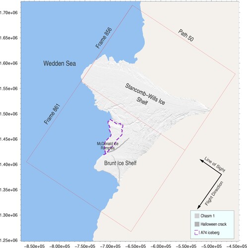
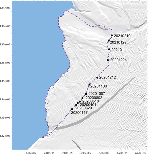
Figure 1 exhibits the study area and the coverage of the input data. The iceberg area, indicated by the purple dashed polygon, is located in the north of the BIS. The Stancomb-Wills Ice Shelf (SWIS) is situated to the north of the BIS. The BIS is a large ice shelf with a dynamic environment in Coats Land and on the eastern coast of the Weddell Sea (King, De Rydt, and Hilmar Gudmundsson 2018), which is the floating extension of the Antarctic ice sheet combining with a series of crevasses. The BIS flows northwestward from the coast with velocities greater than 500 m/a at the calving front although strong temporal variability exists in the flow regime (King, De Rydt, and Hilmar Gudmundsson 2018). Furthermore, there are more than five thousand Emperor Penguins getting along at the SWIS (Fretwell et al. 2012). Two major ruptures, named as Chasm 1 and Halloween crack, are located in the BIS. Halloween crack was initially formed from the McDonald Ice Rumples (MIR) which is a convergence of a series of ice rift. The input data are Sentinel-1 A/B interferometric wide-swath (IW) single look complex (SLC) images acquired from path 50. As a standard Sentinel-1 A/B image cannot well cover BIS and SWIS, the images from frame 856 and 861 are used. The red rectangles in Figure 1 illustrate the coverage of the frames. In total, the area covered by the input data is approximately 120,000 kilometers. The acquisition dates of these images range from 11 January 2020 to 22 February 2021. The Sentinel-1 satellites operate in a near-polar, sun-synchronous orbit with a 12-day repeat cycle. The two-satellite constellation offers a six day exact repeat cycle. Overall, 69 Sentinel-1 A/B acquisitions are utilized for the interferometric analyses.

Figure 1. The study area and the coverage of the input data in polar stereographic projection.

3. 2D velocity field mapping

As mentioned previously, the offset tracking technique is the most widely used method in glacier velocity field mapping applications. Based on this technique, the input Sentinel-1 A/B images are carefully processed in order to depict the temporal evolution of the BIS/SWIS velocity field. To minimize temporal decorrelation, 68 SAR image pairs are formed by consecutive acquisitions. Moreover, a targeted strategy is designed to process the data, which can be mainly partitioned into the following steps:

• Magnitude Alignment: Since the input SAR images are acquired in IW mode, each SLC is stored as three separate sub-swath images. Similar to EnviSAT's ScanSAR data, each sub-swath image is composed of a series of bursts, where each burst is generated as an individual SLC image. To facilitate the application of offset tracking, each SLC is merged into a ‘strip mode’ image by using the corresponding SAR timing information. Note that the offset tracking technique is based on the incoherent cross-correlation (ICC) (Yagüe-Martínez et al. 2016) function; only magnitude images are generated for efficiency concern.

• Geometric Compensation: The image acquired on 1 September 2020 is selected as the master image. For each of the rest images, an offset lookup table with respect to the master image is generated based on ephemeris data and external digital elevation model (DEM) following the idea proposed in Sansosti et al. (2006). Based on such a look-up table, the corresponding magnitude image is resampled to the master's coordinate. In this way, the intrinsic offset induced by the difference in observation geometry is compensated. In the study, the reference elevation model of Antarctica (REMA) (Howat et al. 2019) is used as the external DEM. REMA is obtained based on a large amount of individual stereoscopic DEM extracted from pairs of submeter resolution DigitalGlobe satellite imagery over the austral summer seasons.

• Offset Tracking: The conventional offset tracking method is applied to the resampled magnitude data with respect to each SAR image pairs. The window size is set to 32×128 (azimuth×range). To reduce computational time, the calculation is not carried out on a pixel-by-pixel basis. The intervals between nearby windows are 4 pixels and 12 pixels in the azimuth and the range directions, respectively.

• Quality Evaluation: Due to the presence of temporal decorrelation, unreliable estimates may exist in an offset map. As a glacier velocity field should be distributed continuously, the reliability of the offset measurements in the azimuth and the range directions for a given pixel are assessed separately by using the following root mean square error (RMSE) factor: (1) $RMSE=\frac{\sum _{m=1}^M\sum _{n=1}^N\left[W\right(m,n)-W_{ave}{]}^2}{MN}$(1) where M and N are the predefined window sizes in the azimuth and the range directions (they are both set to 5 in this study), respectively, $W(m,n)$ represents the azimuth/range offset value with respect to the pixel $(m,n)$, and $W_{ave}$ denotes the averaged offset value of the window. When a pixel's RMSE is less than a certain value, either in azimuth or in range, it is marked as an invalid estimate and masked out. Subsequently, the number of valid pixels for each offset map is recorded. An offset map is deleted when the coverage of its valid pixels is less than 70 percentages of the study area. Overall, 33 high-quality offset maps are reserved. The corresponding SAR image pairs are listed in Table 1.

• Interpolation and Lowpass Filter: To fill masked areas, each offset map is interpolated using the consecutive minimization of functionals sequence (CMOFS) algorithm embedded in the open-source surfit software (Mikhail and Vladimir 2021). Subsequently, a lowpass filter is applied to the interpolated data for the purpose of improving the signal-to-noise ratio of the offset measurements.

• Horizontal Displacement Projection: As only ascending Sentinel-1 images were used in this study, the offset tracking technique can only provide the measurements from two directions (azimuth and range). It is assumed that the ice movement in vertical direction is smaller than that in horizontal direction. For the purposed of simplification, the offset vectors in radar coordinate are directly projected into two-dimensional (2D) horizontal displacement vectors in polar stereographic coordinate using the following equation: (2) $\left[\begin{array}{c}{d}_x\\ d_y\end{array}\right]=\left[\begin{array}{c}{d}_{azi}\cos \alpha +d_{ran}\sin \alpha /\sin \theta \\ d_{azi}\sin \alpha -d_{ran}\cos \alpha /\sin \theta \end{array}\right]$(2) where $d_x$ and $d_y$ represent the desired horizontal displacements, $d_{azi}$ and $d_{ran}$ are the offset values in the azimuth and the range directions, respectively, θ is the local incidence angle, and α is the heading angle with respect to the polar stereographic projection. Finally, the horizontal displacements are divided by the temporal baseline, and the 2D glacier velocity maps are thus generated.

Table 1. The high quality SAR image pairs.

ID	SLC1	SLC2	ID	SLC1	SLC2	ID	SLC1	SLC2
1	20200111	20200117	12	20200516	20200522	23	20201112	20201118
2	20200123	20200129	13	20200528	20200603	24	20201124	20201130
3	20200216	20200222	14	20200621	20200627	25	20201206	20201212
4	20200222	20200228	15	20200627	20200703	26	20201218	20201224
5	20200305	20200311	16	20200703	20200709	27	20201224	20201230
6	20200311	20200317	17	20200709	20200715	28	20201230	20210105
7	20200317	20200323	18	20200727	20200802	29	20210105	20210111
8*	20200323	20200329	19	20200802	20200808	30	20210123	20210129
9	20200329	20200404	20	20200814	20200820	31	20210129	20210204
10	20200504	20200510	21	20201001	20201007	32	20210204	20210210
11	20200510	20200516	22	20201019	20201025	33	20210216	20210222

*The master SAR image pairs used in Section 5.

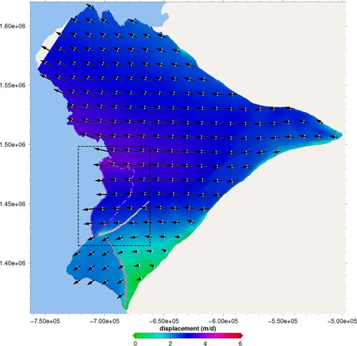
Figure 2 shows the glacier velocity field over BIS and SWIS from 23 March 2020 to 29 March 2020. The black arrows indicate the orientation of the ice flow. It can be observed that the ice flows from the grounding line to the ice front. In addition, the ice flow velocity increases gradually along the flow direction. The ice in most areas flows at a velocity of 2–4 m/d. The peak velocity is observed at intersection area between BIS and SWIS, which is approximately 5 m/d, while the minimum velocity value is located to the right of Chasm-1.

Figure 2. The glacier velocity field with respect to the pair 20200323/20200329.

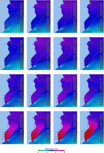
The rest glacier velocity field maps are shown in Figures 3 and 4. Note that the results are presented in separate figures in order to facilitate the type-setting. Moreover, as the aim of this study is to monitor the crack process of the A74 iceberg, only the results in the area indicated by the dashed box in Figure 2 are presented for the clarification purpose. It can be observed that the ice flow velocity over the area of interest remains relatively stable before January 2021. From the end of January 2021, the ice over the A74 area behaves extremely active, as the ice flow velocity arises rapidly. In the result associated with the pair 20210216/20210222, a maximum velocity greater than 6 m/d is observed in the bottom part of the A74 iceberg. As can be seen from the figure, the ice flow direction over non-iceberg area remains generally stable during the whole period of SAR observations. On the other hand, the ice flow orientation over the iceberg region rotates clockwise gradually from the end of December 2020. Moreover, during the period close to the rupture event, in particular at the bottom of the iceberg, the direction of ice flow appears perpendicular to the crack path.

Figure 3. The temporal evolution of the glacier velocity field over the area indicated by the rectangle in Figure 2 (from 11 January 2020 to 15 July 2020).

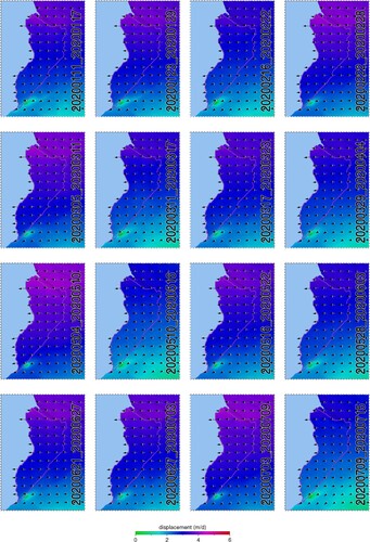
Figure 4. The temporal evolution of the glacier velocity field over the area indicated by the rectangle in Figure 2 (from 27 July 2020 to 22 February 2021).

4. Rift growth tracking

Rift growth mapping is one of the most straightforward methods to monitor an iceberg's activities. Obviously, by using the magnitudes of the input SAR images directly, it is possible to identify the crack extent of the A74 iceberg at each time point of image acquisitions. Note that the resolution of the Sentinel-1A image, in particular in azimuth direction, is relatively low. Since the newly grown rift might be extremely narrow, it is difficult to assure the identification accuracy. One of the possible solutions to improve the accuracy of rift identification is the introduction of optical data (Lai et al. 2020; Shah, Jayaprasad, and James 2019; Xu et al. 2011). Based on this idea, reseachers from ESA derived the rift development of the A74 iceberg between 9 September 2020 and 27 January 2021 by using both Sentinel-1 SAR magnitudes and Sentinel-2 optical images ESA (2021).

From the perspective of radar interferometry, interferometric coherence, which is commonly used for the evaluation of signal quality, might be used as a good criterion for rift identification owing to the following considerations. First, the development of ice rifts indicates the alteration of backscatter signals (Thompson et al. 2020; Marsh et al. 2021). In this case, an inevitable decrease in signal quality will take place. Second, the characteristics of ice shelves should be strongly correlated in space. It implies that continuous coherence observations can be obtained on uncracked ice, which enables the pattern of abnormal ice rifts to be exhibited more distinctly.

Unfortunately, the interferometric signals are generated under a non-stationary scenario due to the rapid motion of ice. The traditional multi-look coherence estimator might be significantly biased as it assumes that the samples are from a circular Gaussian distribution (López-Martínez and Pottier 2007). As presented previously, the ice movement velocity increases gradually from the grounding line to the ice front. In this study, it is assumed that the velocity changing rate does not vary within a small area. In other words, for a given window, the density of interferometric fringes remains constant, which implies that the corresponding signal in the frequency domain follows the pattern of an impulse function. Therefore, the following expression is used to evaluate the quality of the interferometric signals: (3) $\rho =\frac{\left|\mathrm{\Gamma }(p,q)\right|}{\left[\sum _{m=1}^M\sum _{n=1}^N\left|\mathrm{\Gamma }(m,n)\right|-\left|\mathrm{\Gamma }(p,q)\right|\right]/(MN-1)}$(3) where M and N are the number of pixels in each dimension of the window, Γ denotes the Fourier transform of the window, $|\bullet |$ represents a complex number's amplitude, and $(p,q)$ represents the position with the largest amplitude. For the convenience of discussion, ρ is referred to as the signal consistency factor (SCF). In this paper, the window size for SCF calculation is set to 8×8. Note that the window size for the SCF estimation has to be carefully selected. If it is too small, the signal's impulse feature might not be effectively extracted. On the other hand, if a very large window size is used, more computational resources are required. Moreover, the assumption of constant fringe rate might fully break down; thus a severely biased SCF estimate will be obtained.

The calculation of the SCF is based on the interferograms. In this paper, the interferograms are generated generally based on the idea proposed in Scheiber et al. (2014). First, the bursts of all SLC images are resampled based on the original offset look-up table generated in the previous section. To facilitate the discussion, such resampled bursts are referred to as level 1 bursts. For each interferometric pair, the original offset lookup table with respect to SLC 2 is updated based on the corresponding offset tracking result in radar coordinate. The bursts of SLC 2 are resampled again with the use of the updated look-up table, level 2 bursts are therefore obtained. Subsequently, the preliminary burst interferograms are generated based on SLC 1's level 1 bursts and SLC 2's level 2 bursts. To mitigate the problem of phase jump between neighboring bursts, the method described in Wang, Xu, and Fialko (2017) is applied to analyze the preliminary burst interferograms. As a result, the look-up table is further updated, which is used to resample the bursts of SLC 2 to level 3. By merging the burst interferograms with respect to SLC 1's level 1 bursts and SLC 2's level 3 bursts, a monolithic interferogram is finally obtained.

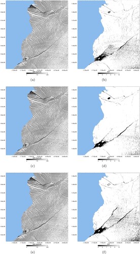
Figure 5(a,c,e) illustrates the SAR amplitude maps acquired on 12 December 2020, from which the Halloween crack can be clearly observed. Moreover, a series of floating ice is observed to the north of the A74 iceberg. This area is known as the Brunt/Stancomb-Wills Chasm (De Rydt et al. 2018). Figure 5(b,d,f) is the SCF maps with respect to the interferometric pair 20201206/20201212. The pattern of the Halloween crack exhibited in this figure is almost identical to that in the SAR amplitude map. The previous discussion about the signal characteristics of newly grown rifts is confirmed by the patterns of the A74 crack presented in the SAR amplitude map and the SCF map. In the SAR amplitude map, the pattern of the A74 rift is shallow and short. In contrast, the pattern is obvious in the SCF map as the rift is newly grown. Note that the SCF value over the MIR area is extremely low. As mentioned previously, MIR is a convergence of a series of ice ruptures. The high shear strain rate is believed to be the chief reason causing such low SCF values.

Figure 5. The comparison between SAR amplitude maps and SCF maps. The SAR amplitude maps acquired on (a) 20200727, (c) 20201001 and (e) 20201206; (b) The SCF maps with respect to the interferometric pairs (a) 20200727/202008002, (c) 20201001/20201007 and (e) 20201206/20201212.

The SCF map with respect to each high-quality interferometric pair is generated for the purpose of rift growth tracking. Twelve representative rift front ends in different times are labeled, a rift growth path is therefore generated, as shown in Figure 6. It is compared with the rift growth path presented in ESA (2021), which is obtained by ESA using both Sentinel-1 SAR magnitudes and Sentinel-2 optical images. In general, the SCF-based rift growth path is generally similar to the ESA's result. The effectiveness of the proposed SCF is therefore proved. However, there are several differences that can be discussed in detail. First, Figure 6 gives a more detailed view of the trend of the A74 calving process over a year, whereas only the rift growth path between 9 September 2020 and 27 January 2021 is contained in the ESA result. Second, the rift front end from the SCF result is slightly ahead of/behind that from the ESA's result in October/November.

Figure 6. The ice crack growth path obtained from the SCF maps.

5. Interferometric phase change detection

Based on the results represented in previous sections, it is reasonable to assume that the temporal evolution of the flow behavior of the A74 iceberg follows the pattern depicted in Figure 7, which can be separated into two stages. First, the iceberg flows in a relatively steady state, as no evident variation of its displacement velocity is presented. During the second stage, the flow of the iceberg is speeding up exponentially as time goes on. In other words, the iceberg acts in an unsteady state, which indicates that the complete rupture of the iceberg might take place within a short period. In this paper, the intersection of the two stages is referred to as the state transition point (STP). Evidently, the STP can be treated as a precursor signal of the final iceberg crack event.

Figure 7. The hypothetical temporal evolution pattern of an iceberg.

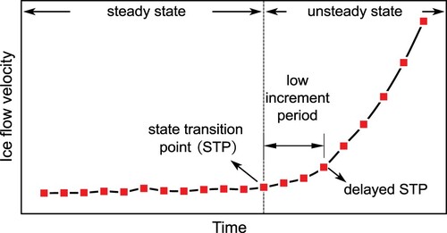
According to the velocity field obtained from the offset tracking technique, it can be considered that the STP is around the middle of January 2021, as there is a clear variation between the results associated with the pair 20210105/20210111 and 20210123/20210129. It is well known that the offset tracking technique can only achieve a sub-pixel level measurement accuracy (Zhang et al. 2019). The range and the azimuth resolutions of a standard IW Sentinel-1A/B SLC image are approximately 5 m and 20 m (Dong et al. 2021), respectively. On the ground that the offset tracking technique aims to measure the projections of horizontal ice movement vectors onto the range and the azimuth directions, it can be considered that the results associated with Figures 2–4 can only reflect meter-level ice displacements. Note that the ice flow velocity grows in an exponential manner, which implies that there is a ‘low increment period’ after the STP. Due to the low accuracy of the offset tracking results, the increment phenomenon during this period may not be effectively aware. Where this is the case, a delayed STP might be determined (see Figure 7). To mitigate this problem, an interferometric phase-based method is developed for the purpose of STP determination.

The 33 differential interferograms generated in the previous section are firstly used to form an interferogram stack. For a given position $(x,y)$, the phase in the ith interferogram can be denoted as (Zhang et al. 2013): (4) ${\phi }^i(x,y)={\phi }_{disp}^i(x,y)+{\phi }_{derr}^i(x,y)+{\phi }_{atm}^i(x,y)+{\phi }_{noise}^i(x,y)$(4)

• ${\phi }_{disp}^i(x,y)$ refers to the phase induced by glacier flow, which can be further expressed as (Ferretti, Prati, and Rocca 2000): (5) ${\phi }_{disp}^i(x,y)=-\frac{4\pi }{\lambda }{l}^i(x,y)$(5) where λ represents the radar wavelength and $l^i(x,y)$ illustrates the ice surface displacement occurring between the image acquisitions with respect to the ith interferogram. For the Sentinel-1 A/B case, λ is approximately 5.6 cm. Therefore, when $l^i(x,y)$ is 28 m (approximately 4.5 m/d), the phase contributed by the glacier activities can achieve 2000π rad, which corresponds to 1000 interferometric fringes from a stable point to $(x,y)$.

• ${\phi }_{derr}^i(x,y)$ is the residual phase contributed by an inaccuracy in the external DEM, which can be denoted as (Berardino et al. 2002): (6) ${\phi }_{derr}^i(x,y)=-\frac{4\pi }{\lambda }\frac{B_{\mathrm{\perp }}^i(x,y)}{R(x,y)\cdot \sin \theta (x,y)}{h}^i(x,y)$(6) where $B_{\mathrm{\perp }}^i(x,y)$ is the perpendicular baseline of the ith interferogram, $R(x,y)$ is the distance between the sensor to the target along the line-of-sight (LOS) direction, $\theta (x,y)$ is the local incidence angle and $h^i(x,y)$ is the DEM error. For the case of glacier monitoring applications, $h^i(x,y)$ can be considered to be composed of two items: (7) $h^i(x,y)=h_c(x,y)+h_f^i(x,y)$(7) where $h_c(x,y)$ is the connatural error contained in the external DEM and $h_f^i(x,y)$ is the DEM change induced by ice movements (Sun et al. 2017), respectively. In order to preserve interferometric coherence, the orbit positioning control of Sentinel-1 A/B is very stringent, which makes $B_{\mathrm{\perp }}^i(x,y)$ smaller than 100 m in most cases. It means that a 5 m connatural DEM error will only lead to a phase approximately less than 0.068π rad under a general Sentinel-1 A/B imaging geometry $R(x,y)=850$ km and $\theta (x,y)={38}^{\circ }$. Therefore, it is reasonable to assume that $h_c(x,y)$ is negligible in this paper's application.

• ${\phi }_{atm}^i(x,y)$ is the phase contributed by atmospheric disturbances.

• ${\phi }_{noise}^i(x,y)$ represents decorrelation noise. In this paper, the conventional Goldstein phase filter method (Goldstein and Werner 1998; Baran et al. 2003) is applied to all interferograms to suppress this item. The corresponding window size is set to $16\times 16$.

In this paper, the idea of change detection is applied to the interferograms for the purpose of STP determination. First, the quality of each interferogram is evaluated by the sum of each pixel's interferometric coherence. The interferogram with the best quality (pair 20200323/20200329) is selected as the reference interferogram in order to assure the maximization of the quality of change detection results. To obtain the interferometric signal change, the most straightforward method is to directly generate the double-differential interferograms by simply applying conjugate multiplication to the other interferograms and the reference interferogram. However, it will lead to the following two problems. (a) As interferometric phase can be only expressed in modulo 2π rad, it must be integrated to generate unwrapped observations (Goldstein, Zebker, and Werner 1988). In glacier applications, a repeat-pass interferogram is very likely to be separated into isolated fringe regions due to shear margins of ice streams and other low-coherence zones (Liu, Zhao, and Jezek 2007). Where this is the case, it is hard to obtain a complete phase unwrapping result unless a previously measured point is available for each region. (b) Since $h_f^i(x,y)$ and ${\phi }_{atm}^i(x,y)$ are varying over time, the phase subtraction operation could not diminish their negative impacts on the displacement signals. In this paper, the change in phase gradient is calculated in order to mitigate the above problems. For a given position, the phase gradient vector on the ith interferogram is calculated by: (8) ${\mathbf{g}}^i(x,y)=\left[\begin{array}{c}Wrap\left({\phi }^i(x+1,y)-{\phi }^i(x,y)\right)\\ Wrap\left({\phi }^i(x,y+1)-{\phi }^i(x,y)\right)\end{array}\right]$(8) where $Wrap(\bullet )$ indicates the phase wrapping operation. Based on the above discussion, it can be further expressed as: (9) ${\mathbf{g}}^i(x,y)=\left[\begin{array}{c}Wrap\left({\delta }_x^i(x,y)+{\eta }_x^i(x,y)+{\alpha }_x^i(x,y)\right)\\ Wrap\left({\delta }_y^i(x,y)+{\eta }_y^i(x,y)+{\alpha }_y^i(x,y)\right)\end{array}\right]$(9) where (10) $\begin{array}{rl}{\delta }_x^i(x,y)& ={\phi }_{disp}^i(x+1,y)-{\phi }_{disp}^i(x,y),{\delta }_y^i(x,y)={\phi }_{disp}^i(x,y+1)-{\phi }_{disp}^i(x,y)\\ {\eta }_x^i(x,y)& =-\frac{4\pi }{\lambda }\frac{B_{\mathrm{\perp }}^i(x,y)}{R(x,y)\cdot \sin \theta (x,y)}\left[h_f^i(x+1,y)-h_f^i(x,y)\right]\\ {\eta }_y^i(x,y)& =-\frac{4\pi }{\lambda }\frac{B_{\mathrm{\perp }}^i(x,y)}{R(x,y)\cdot \sin \theta (x,y)}\left[h_f^i(x,y+1)-h_f^i(x,y)\right]\\ {\alpha }_x^i(x,y)& ={\phi }_{atm}^i(x+1,y)-{\phi }_{atm}^i(x,y),{\alpha }_y^i(x,y)={\phi }_{atm}^i(x,y+1)-{\phi }_{atm}^i(x,y)\end{array}$(10) Note that atmospheric phase contributions exhibit a low-wavenumber spectral behavior (Ferretti, Prati, and Rocca 2001). As a result, the atmosphere induced signals on neighboring resolution elements can be considered to be identical to each other, implying that ${\alpha }_{\ast }^i(x,y)$ is zero. Moreover, it is reasonable to assume that the DEM change due to glacier flow remains constant within a small area. That is to say, ${\eta }_{\ast }^i(x,y)$ is negligible. Therefore, it can be considered that: (11) $\begin{array}{rl}{\phi }^i(x+1,y)-{\phi }^i(x,y)& \approx {\phi }_{disp}^i(x+1,y)-{\phi }_{disp}^i(x,y)\\ {\phi }^i(x,y+1)-{\phi }^i(x,y)& \approx {\phi }_{disp}^i(x,y+1)-{\phi }_{disp}^i(x,y)\end{array}$(11) According to the phase unwrapping theory (Goldstein, Zebker, and Werner 1988), if all true phase gradients are assumed to be less than π rad (referred to as phase gradient assumption), wrapped phase gradients are equal to true phase gradients. In this case, the following expressions hold everywhere: (12) $\begin{array}{rl}Wrap\left({\phi }^i(x+1,y)-{\phi }^i(x,y)\right)& ={\phi }^i(x+1,y)-{\phi }^i(x,y)\\ Wrap\left({\phi }^i(x,y+1)-{\phi }^i(x,y)\right)& ={\phi }^i(x,y+1)-{\phi }^i(x,y)\end{array}$(12) This equation indicates that the phase unwrapping of ${\mathbf{g}}^i(x,y)$ is unnecessary. Therefore, the change in interferometric phase gradient can be directly obtained by: (13) ${\mathbf{c}}^i(x,y)={\mathbf{g}}^i(x,y)-{\mathbf{g}}^r(x,y)$(13) where r indicates the index of the reference interferogram. As indicated previously, the ice over the study area could flow very rapidly, which implies that the fringe density of the interferograms could be very high. If a large multi-look factor is used for interferogram generation, phase signal saturation (Ge, Chang, and Rizos 2007) might take place in the majority of areas, leading to the phase gradient assumption being invalid. To make the utmost possible amount of pixels satisfy the assumption, the interferograms are only multi-looked in range direction using a factor of 3. The purpose of such a multi-look operation is merely to balance the grid sizes in the azimuth and the range directions.

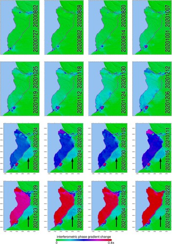
Figures 8 and 9 show the resulting phase gradient change maps. Note that the interferometric phase gradient change expressed in Equation (13(13) ${\mathbf{c}}^i(x,y)={\mathbf{g}}^i(x,y)-{\mathbf{g}}^r(x,y)$(13) ) is a complex number. During the period of observation, the variation in its phase is relatively small. Therefore, only the magnitude of phase gradient change on each pixel is presented. Moreover, as the interferometric signals are only correlated with the ground surface displacements in the LOS direction, no arrows indicating 2D ice flow direction are presented in these figures. According to these figures, the steady state and the unsteady state of the A74 iceberg can be generally separated. It can be considered that the STP is located at the beginning of December 2020, which is around one month earlier than that deduced from the offset tracking results. During the period before the STP, no changes can be obviously observed from the results except for MIR and Brunt/Stancomb-Wills Chasm. For the MIR case, the presence of such changes is believed caused by the sea water contained in ice gaps. On the other hand, the singular signals in the area of Brunt/Stancomb-Wills Chasm may stem from the movements of floating ice. When the state of the iceberg is altered to unsteady, abnormal phase change signals are clearly observed. Moreover, the pattern of the abnormal signals is nearly identical to the extent of the A74 iceberg (as indicated by the purple dashed polygon). It indicates that the scale of the A74 iceberg can be predicted approximately two and half months before the final rupture event.

Figure 8. The interferometric phase gradient change maps (from 11 January 2020 to 15 July 2020).

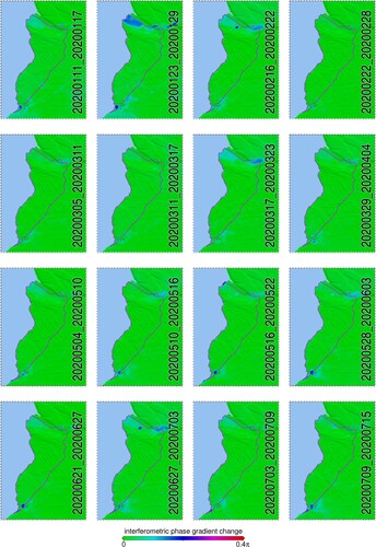
Figure 9. The interferometric phase gradient change maps (from 27 July 2020 to 22 February 2021).

From the middle of December 2020, relatively small abnormal signals can be observed over the region between Halloween crack and the A74 iceberg rift, as indicated by the black arrow. Such signals cannot be observed from the offset tracking result. Therefore, the proposed method's advantage in sensitivity compared to the offset tracking technique is further confirmed to some extent. Note that these signals tend to disappear from the beginning of February 2021. This phenomenon can be explained as follows. Between the middle of December 2020 and the beginning of February 2021, the contact between A74 and BIS was relatively intense. The ice over the area closed to the iceberg was pulled by the force induced by the iceberg movement. On the other hand, the connection between A74 and BIS became remarkably weak, during the period extremely closed to the final crack event. This is the main reason that why such signals are difficultly observed in the last two results in Figure 9.

6. Conclusion

With the use of the pre-event Sentinel-1 A/B SAR images, the crack process of the Antarctic A74 iceberg is monitored in different aspects based on the idea of radar interferometry in this study. The temporal evolution of the ice flow velocity field is firstly derived based on a well-designed offset tracking strategy. Next, the interferograms with respect to high quality interferometric pairs are generated. For each interferogram, the SCF is defined and calculated to map the crack extent. Compared to the SAR magnitude images, the SCF maps can exhibit a much clearer rupture pattern, which leads to a more precise presentation of the crack's growth process. Lastly, a new change detection method is proposed to further reveal the temporal evolution of the iceberg. Compared to the offset tracking technique, this method is more sensitive to ice flow activities as it is based on interferometric phase signals, implying that the abnormal variation of the iceberg can be identified in an earlier stage.

It can be observed from the offset tracking results that the ice flow velocity of the A74 iceberg increases rapidly before the event of the rupture. In the meanwhile, the orientation of the velocity vectors over the iceberg areas tends to be perpendicular to the crack path. Therefore, it is believed that there is a mutual response effect during the crack process of the A74 iceberg: The initial loss of contact between A74 and BIS triggers a change in flow velocity and orientation of the iceberg. On the other hand, the force caused by such a change sharpens the rupture process, which further weakens the connection between A74 and BIS. The offset tracking results also demonstrate that the iceberg was extremely active in February 2021. However, according to the rift growth map shown in Figure 6, the rift extent change occurring during this period is relatively small. The rift growth information obtained from the proposed method can only exhibit the surface status of glaciers. Therefore, it is believed that the process of an iceberg's generation cannot be correctly depicted by purely using surface rift information. According to the change detection results from Figures 8 and 9, it can be considered that the abnormal behavior of the ice flow took place at the beginning of December 2020. Moreover, the distribution of the abnormal signals is almost identical to that of the cracked region, which indicates that it is possible to predict the scale of the iceberg approximately 70 days before the final crack event. Such a prediction capability is the most distinct advantage of the proposed change detection method. Note that the abnormal signals over the iceberg region appear a consistent pattern. Therefore, it is reasonable to consider that the contact between the iceberg and BIS was losing in a global sense rather than a local sense. In addition, such a consistent pattern might indicate that the ice flow mechanism was altered. Where this is the case, the complete crack of the corresponding ice body is inevitable.

Disclosure statement

No potential conflict of interest was reported by the author(s).

Data availability statement

The data used in this paper are publicly available and can be obtained from the following links:

The Sentinel-1 A/B data are available at https://search.asf.alaska.edu.

The REMA data are available at https://www.pgc.umn.edu/data/rema.

Additional information

Funding

This research was funded by Chongqing Basic Science And Frontier Technology Research Project [grant number 2017jcyjAX0229] and China Postdoctoral Science Foundation [grant number 2019M660022XB].

References

- Baran, Ireneusz, Mike P. Stewart, Bert M. Kampes, Zbigniew Perski, and Peter Lilly. 2003. “A Modification to the Goldstein Radar Interferogram Filter.” IEEE Transactions on Geoscience and Remote Sensing 41 (9): 2114–2118.
- BBC News. 2021a. “Antarctic Seafloor Exposed after 50 Years of Ice Cover.” Accessed 25 March 2021. https://www.bbc.com/news/science-environment-56424338.
- BBC News. 2021b. “Brunt Ice Shelf: Big Iceberg Calves near UK Antarctic Base.” Accessed 25 March 2021. https://www.bbc.com/news/science-environment-47692895.
- BBC News. 2021c. “Iceberg A-74 Calves from the Brunt Ice Shelf in the Weddell Sea.” Accessed 25 March 2021. https://usicecenter.gov/PressRelease/IcebergA74.
- BBC News. 2021d. “Mega-Iceberg A74: German Ship Squeezes through Narrow Ice Channel.” Accessed 25 March 2021. https://www.bbc.com/news/science-environment-56404142.
- BBC News. 2021e. “Radar Images Capture New Antarctic Mega-Iceberg.” Accessed 25 March 2021. https://www.bbc.com/news/science-environment-56241503.
- Berardino, Paolo, Gianfranco Fornaro, Riccardo Lanari, and Eugenio Sansosti. 2002. “A New Algorithm for Surface Deformation Monitoring Based on Small Baseline Differential SAR Interferograms.” IEEE Transactions on Geoscience and Remote Sensing 40 (11): 2375–2383.
- Doman, Mark. 2021. “The Birth of a Mega Antarctic Iceberg.” Accessed 25 March 2021. https://www.abc.net.au/news/2021-03-05/satellites-capture-birth-of-brunt-ice-shelf-antarctic-iceberg/13208776?nw=0.
- Dong, Jie, Shangjing Lai, Nan Wang, Yian Wang, Lu Zhang, and Mingsheng Liao. 2021. “Multi-Scale Deformation Monitoring with Sentinel-1 InSAR Analyses along the Middle Route of the South-North Water Diversion Project in China.” International Journal of Applied Earth Observation and Geoinformation 100: 102324.
- ESA. 2021. “Is Brunt on the Brink?” Accessed 25 March 2021. https://www.esa.int/Applications/Observing_the_Earth/Copernicus/Is_Brunt_on_the_brink.
- Ferretti, Alessandro, Claudio Prati, and Fabio Rocca. 2000. “Nonlinear Subsidence Rate Estimation Using Permanent Scatterers in Differential SAR Interferometry.” IEEE Transactions on Geoscience and Remote Sensing 38 (5): 2202–2212.
- Ferretti, Alessandro, Claudio Prati, and Fabio Rocca. 2001. “Permanent Scatterers in SAR Interferometry.” IEEE Transactions on Geoscience and Remote Sensing 39 (1): 8–20.
- Fretwell, Peter T., Michelle A. LaRue, Paul Morin, Gerald L. Kooyman, Barbara Wienecke, Norman Ratcliffe, Adrian J. Fox, et al. 2012. “An Emperor Penguin Population Estimate: The First Global, Synoptic Survey of a Species from Space.” PloS One 7 (4): e33751.
- Ge, Linlin, Hsing-Chung Chang, and Chris Rizos. 2007. “Mine Subsidence Monitoring Using Multi-Source Satellite SAR Images.” Photogrammetric Engineering & Remote Sensing 73 (3): 259–266.
- Goldstein, Richard M., and Charles L. Werner. 1998. “Radar Interferogram Filtering for Geophysical Applications.” Geophysical Research Letters 25 (21): 4035–4038.
- Goldstein, Richard M., Howard A. Zebker, and Charles L. Werner. 1988. “Satellite Radar Interferometry: Two-Dimensional Phase Unwrapping.” Radio Science 23 (4): 713–720.
- Gomez, Rodrigo, Jorge Arigony-Neto, Angela De Santis, Saurabh Vijay, Ricardo Jaña, and Andres Rivera. 2019. “Ice Dynamics of Union Glacier from SAR Offset Tracking.” Global and Planetary Change174: 1–15.
- Hogg, Anna E., and G. Hilmar Gudmundsson. 2017. “Impacts of the Larsen-C Ice Shelf Calving Event.” Nature Climate Change 7 (8): 540–542.
- Howat, Ian M., Claire Porter, Benjamin E. Smith, Myoung-Jong Noh, and Paul Morin. 2019. “The Reference Elevation Model of Antarctica.” The Cryosphere 13 (2): 665–674.
- King, Edward C., Jan De Rydt, and G. Hilmar Gudmundsson. 2018. “The Internal Structure of the Brunt Ice Shelf from Ice-Penetrating Radar Analysis and Implications for Ice Shelf Fracture.” The Cryosphere12 (10): 3361–3372.
- Lai, Ching-Yao, Jonathan Kingslake, Martin G. Wearing, Po-Hsuan Cameron Chen, Pierre Gentine, Harold Li, Julian J. Spergel, and J. Melchior van Wessem. 2020. “Vulnerability of Antarctica's Ice Shelves to Meltwater-Driven Fracture.” Nature 584 (7822): 574–578.
- Liu, Hongxing, Zhiyuan Zhao, and Kenneth C. Jezek. 2007. “Synergistic Fusion of Interferometric and Speckle-Tracking Methods for Deriving Surface Velocity from Interferometric SAR Data.” IEEE Geoscience and Remote Sensing Letters 4 (1): 102–106.
- López-Martínez, Carlos, and Eric Pottier. 2007. “Coherence Estimation in Synthetic Aperture Radar Data Based on Speckle Noise Modeling.” Applied Optics 46 (4): 544–558.
- Marsh, O. J., D. Price, Z. R. Courville, and Dana Floricioiu. 2021. “Crevasse and Rift Detection in Antarctica from TerraSAR-X Satellite Imagery.” Cold Regions Science and Technology 187: 103284.
- Mikhail, Dmitrievskiy, and Kutrunov Vladimir. 2021. “Surfit Docs.” Accessed 25 March 2021. http://surfit.sourceforge.net/surfit/index.html.
- NASA Earth Observatory. 2021. “Breakup at Brunt.” Accessed 25 March 2021. https://earthobservatory.nasa.gov/images/148009/breakup-at-brunt.
- Riveros, N., L. Euillades, P. Euillades, S. Moreiras, and Sebastian Balbarani. 2013. “Offset Tracking Procedure Applied to High Resolution SAR Data on Viedma Glacier, Patagonian Andes, Argentina.” Advances in Geosciences 35: 7–13.
- De Rydt, Jan, G. Hilmar Gudmundsson, Thomas Nagler, Jan Wuite, and Edward C. King. 2018. “Recent Rift Formation and Impact on the Structural Integrity of the Brunt Ice Shelf, East Antarctica.” The Cryosphere 12 (2): 505–520.
- Sánchez-Gámez, Pablo, and Francisco J. Navarro. 2017. “Glacier Surface Velocity Retrieval Using D-InSAR and Offset Tracking Techniques Applied to Ascending and Descending Passes of Sentinel-1 Data for Southern Ellesmere Ice Caps, Canadian Arctic.” Remote Sensing 9 (5): 442.
- Sansosti, Eugenio, Paolo Berardino, Michele Manunta, Francesco Serafino, and Gianfranco Fornaro. 2006. “Geometrical SAR Image Registration.” IEEE Transactions on Geoscience and Remote Sensing 44 (10): 2861–2870.
- Scheiber, Rolf, Marc Jäger, Pau Prats-Iraola, Francesco De Zan, and Dirk Geudtner. 2014. “Speckle Tracking and Interferometric Processing of TerraSAR-X TOPS Data for Mapping Nonstationary Scenarios.” IEEE Journal of Selected Topics in Applied Earth Observations and Remote Sensing 8 (4): 1709–1720.
- Shah, Esha, P. Jayaprasad, and M. E. James. 2019. “Image Fusion of SAR and Optical Images for Identifying Antarctic Ice Features.” Journal of the Indian Society of Remote Sensing 47 (12): 2113–2127.
- Shugar, Dan H., Bernhard T. Rabus, John J. Clague, and Denny M. Capps. 2012. “The Response of Black Rapids Glacier, Alaska, to the Denali Earthquake Rock Avalanches.” Journal of Geophysical Research: Earth Surface 117: F01006.
- Strozzi, Tazio, Adrian Luckman, Tavi Murray, Urs Wegmuller, and Charles L. Werner. 2002. “Glacier Motion Estimation Using SAR Offset-Tracking Procedures.” IEEE Transactions on Geoscience and Remote Sensing 40 (11): 2384–2391.
- Sun, Yafei, Liming Jiang, Lin Liu, Qishi Sun, Hansheng Wang, and Houtse Hsu. 2017. “Mapping Glacier Elevations and their Changes in the Western Qilian Mountains, Northern Tibetan Plateau, by Bistatic InSAR.” IEEE Journal of Selected Topics in Applied Earth Observations and Remote Sensing 11 (1): 68–78.
- Thompson, S. S., S. Cook, B. Kulessa, J. Paul Winberry, A. D. Fraser, and B. K. Galton-Fenzi. 2020. “Comparing Satellite and Helicopter-Based Methods for Observing Crevasses, Application in East Antarctica.” Cold Regions Science and Technology 178: 103128.
- Wang, Qun, Jinghui Fan, Wei Zhou, Liqiang Tong, Zhaocheng Guo, Guang Liu, Weilin Yuan, Joaquim João Sousa, and Zbigniew Perski. 2019. “3D Surface Velocity Retrieval of Mountain Glacier Using an Offset Tracking Technique Applied to Ascending and Descending SAR Constellation Data: A Case Study of the Yiga Glacier.” International Journal of Digital Earth 12 (6): 614–624.
- Wang, Kang, Xiaohua Xu, and Yuri Fialko. 2017. “Improving Burst Alignment in TOPS Interferometry with Bivariate Enhanced Spectral Diversity.” IEEE Geoscience and Remote Sensing Letters 14 (12): 2423–2427.
- Wild, Christian T., Oliver J. Marsh, and Wolfgang Rack. 2018. “Unraveling InSAR Observed Antarctic Ice-Shelf Flexure Using 2-D Elastic and Viscoelastic Modeling.” Frontiers in Earth Science 6: 28.
- Xu, Tao, Wen Yang, Ying Liu, Chunxia Zhou, and Zemin Wang. 2011. “Crevasse Detection in Antarctica using ASTER Images.” In International Conference Image Analysis and Recognition, 370–379. Springer.
- Yagüe-Martínez, Néstor, Pau Prats-Iraola, Fernando Rodriguez Gonzalez, Ramon Brcic, Robert Shau, Dirk Geudtner, Michael Eineder, and Richard Bamler. 2016. “Interferometric Processing of Sentinel-1 TOPS Data.” IEEE Transactions on Geoscience and Remote Sensing 54 (4): 2220–2234.
- Zhang, Kui, Linlin Ge, Xiaojing Li, and Alex Hay-Man Ng. 2013. “Monitoring Ground Surface Deformation Over the North China Plain Using Coherent ALOS PALSAR Differential Interferograms.” Journal of Geodesy 87 (3): 253–265.
- Zhang, Kui, Faming Gong, Zhiyong Li, Shujun Liu, and Yuhan Shen. 2019. “Recover Glacier Velocity Fields Derived from the SAR Speckle Tracking Technique Using Artificial Neural Network.” IEEE Geoscience and Remote Sensing Letters 16 (8): 1250–1253.