Mapping mountain glaciers using an improved U-Net model with cSE

ABSTRACT

Global warming is melting glaciers. Changes in mountain glaciers have a tremendous impact on human life. Regular identification and extraction of glaciers from satellite images are necessary. However, when studying glaciers, materials surrounding the glacier have high spectral similarity to glaciers and are easily misclassified in the identification process. Therefore, in this study of glacier extraction, we used an improved U-Net model (a channel-attention U-Net) to map glaciers. The model was trained on Landsat 8 Operational Land Imager (OLI) data and a Shuttle Radar Topography Mission (SRTM) digital elevation model (DEM), and was tested on glaciers in the Pamir Plateau. The results show that the channel-attention U-Net identifies glaciers with relatively high accuracy compared to U-Net and GlacierNet. The obtained results were fine-tuned by the conditional random field model, effectively reducing background misidentification.

KEYWORDS:

• U-Net
• channel-attention mechanism
• conditional random field
• glacier extraction
• Pamir Plateau

1. Introduction

Glaciers, the largest freshwater resource in the world, are sensitive to climate change (Paul et al. 2015). Against the background of climate warming, glaciers worldwide are gradually retreating and melting (Zemp et al. 2015). In addition to causing sea level rise (Gardner et al. 2013), changes in mountain glaciers can lead to natural disasters such as floods, mudslides, and landslides (Raper and Braithwaite 2006; Raup et al. 2015; Wang et al. 2011). Accurate detection of the changing characteristics of mountain glaciers is important in reducing the impact of glacial hazards.

Traditional glacier survey methods require field visits, but this is time-consuming and it is difficult to survey a large area. Monitoring methods based on remote sensing images can obtain the spatial distribution of glaciers quickly and accurately with low cost, so they have become a hot research topic for glacier monitoring (Zemp et al. 2015; Raup, Kääb, et al. 2007; Nie, Liu, and Liu 2013). In particular, Landsat data, which has the advantages of a long coverage period, high spectral resolution, and wide coverage, is an important data source for glacier monitoring on a large scale (Bolch, Menounos, and Wheate 2010; Paul et al. 2016; Mölg et al. 2018). Currently, methods for identifying glaciers mainly include the band ratio threshold method (Burns and Nolin 2014; Singh et al. 2021), normalized-difference snow index (NDSI) (Salomonson and Appel 2006), supervised classification methods (Pope and Rees 2014), unsupervised classification methods (Gjermundsen et al. 2011; Paul 2002), object-based image analysis (OBIA) methods (Karimi et al. 2015), and neural network classification methods (Baumhoer et al. 2019; Xie et al. 2020). The band ratio method and NDSI method extract glaciers automatically or semi-automatically (Wang et al. 2020) by setting thresholds through the combination of glacier-sensitive feature bands in a mathematical operation. However, this method can only effectively extract clean glacier areas, and the accuracy depends heavily on the selection of the thresholds (Singh et al. 2021). The object-oriented classification method is cumbersome to operate. Its accuracy depends on the establishment of knowledge rules (Bishop et al. 2001). The accuracy of supervised classification is higher than that of unsupervised classification. However, due to complex scenarios such as cloud shadows, mountain shadows, and similarity of spectral features generated by water icing, it is difficult to achieve better robustness and higher accuracy using the above methods.

Deep learning methods can automatically learn features from samples and can train and predict end-to-end. They have achieved good results in remote sensing image feature extraction and have gradually been applied to glacier studies in recent years. Mohajerani et al. (Mohajerani et al. 2019) used a U-Net deep learning semantic segmentation network (Ronneberger, Fischer, and Brox 2015) to extract glacier break lines at different scales. Nijhawan et al. (Nijhawan, Das, and Balasubramanian 2018) used multiple convolutional neural networks (CNNs) to extract features from Landsat 8 multispectral band data, topography, and texture parameters. A random forest classifier then classified these features to achieve the classification of debris-covered glaciers. Zhang et al. (Zhang, Liu, and Huang 2019) automatically depicted the calving front positions of Jakobshavn Isbrae from 2009 to 2015 by applying U-Net to multi-temporal synthetic aperture radar images acquired by the TerraSAR-X satellite. They also found that the calving fronts retreated. Xie et al. (Xie et al. 2020) designed GlacierNet to extract highly accurate debris-covered glacier boundaries from Landsat 8 images, digital elevation models (DEMs), and surface parameters derived from DEMs. Robson et al. (Robson et al. 2020) used a convolutional neural network to obtain predicted heat maps based on Sentinel-2 optical images, Sentinel-1 interferometric coherence data, and DEMs. The heat maps were then segmented and classified using OBIA. Cheng et al. (Cheng et al. 2021) developed the Calving Front Machine (CALFIN), an automated method that used deep learning to automate the extraction of calving fronts from satellite imagery, with results often indistinguishable from manually labeled fronts. Zhang et al. (Zhang et al. 2021) evaluated four neural network architectures (e.g. U-Net, DeepLabv3+ with ResNet, DRN, and MobileNet as the backbone) and three histogram modification strategies using seven remote sensing datasets of optical and synthetic aperture radar images. Among them, the combination of histogram normalization and DRN-DeepLabv3+ had the lowest test error.

The semantic segmentation model U-Net was initially used in biomedical image segmentation and has also achieved good results in the semantic segmentation of remote sensing images, such as building segmentation (Abdollahi, Pradhan, and Alamri 2020) and road extraction (Sofla, Alipour-Fard, and Arefi 2021). In recent years, more and more scholars have applied the U-Net model to the field of glacier research with high accuracy. Jamil et al. (Jamil et al. 2019) showed that the U-Net model effectively detects glacier changes. He et al. (He et al. 2020) also used Deep U-Net to identify glaciers in Landsat 8 OLI images, and the results showed that U-Net can exclude water bodies and shadow areas well.

In this study, we propose a U-Net semantic segmentation network that incorporates a channel-attention mechanism to better distinguish the spectral differences between glaciers and non-glaciers and thus extract glaciers from the remote sensing images with higher accuracy. In addition, the conditional random field (CRF) method is used to post-process the extraction results, which effectively solves the ‘noise’ and ‘hole’ problems. Experiments based on Landsat 8 data and DEM data are conducted and compared with other methods to verify the effectiveness.

2. Study sites and data

2.1. Study area

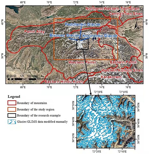
The Pamir Plateau (Mölg et al. 2018; Gardelle et al. 2013), spanning southwestern Xinjiang, southeastern Tajikistan, and northeastern Afghanistan, is the intersection of the Kunlun, Karakorum, Hindu Kush, and Tian Shan mountains. The average altitude is over 4,500 meters. The Pamir Plateau has an alpine climate. More than 1,000 mountain glaciers cover an area of nearly 10,000 square kilometers. In particular, the Fedchenko Glacier is one of the largest mountain glaciers in the world. The study area is part of eastern Pamir, western Pamir, and Pamir-Alay, with a geographical position between 37°48’N-40°2’N and 70°22’E-76°41’E (Figure 1).

Figure 1. Location of the Pamir study area and examples of glaciers studied.

2.2. Data

In the study, freely available Landsat 8 OLI data and SRTM DEM data (Van Zyl 2001), available from the United States Geological Survey (USGS) website (https://earthexplorer.usgs.gov/), were used. Landsat 8 OLI images were selected during the summer of 2019 to minimize the effect of seasonal snowfall on glacier extent. Meanwhile, it was ensured that images had less cloud cover. The Landsat 8 image was corrected, stretched, resampled to 15 m, and a three-band false-color composite image was obtained. The SRTM DEM data product is SRTM 1 Arc-Second Global with a spatial resolution of 30 m. The DEM was also resampled to 15 m spatial resolution using the nearest neighbor method to match the Landsat 8 image. The glacier boundary shapefiles from the Global Land Ice Measurements from Space (GLIMS) database (Raup, Racoviteanu, et al. 2007) (http://www.glims.org) were modified as groundtruths. Since there is a temporal gap between the GLIMS data and the data we used, and glacier boundary contours are subject to change, the GLIMS data were manually modified to ensure the label's accuracy. Specifically, GLIMS data were combined with hand-drawn glacier data, since some of our manually drawn boundaries were coarse.

3. Method

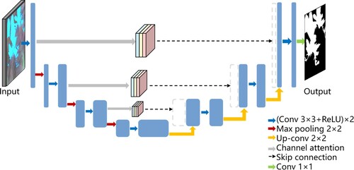
Deep learning is an important branch of machine learning. Deep learning builds neural networks that simulate the analysis and learning of the human brain to recognize data such as images, sounds, and text. It has gradually been applied to remote sensing image research in recent years, such as target recognition (Huang, Pan, and Lei 2020), scene classification (Cheng, Han, and Lu 2017), and change detection (Zhang, Zhang, and Du 2016). As an important research direction in computer vision, semantic segmentation can be implemented to classify each pixel. Therefore, in this study, we will use a semantic segmentation network to extract glacier regions. Widely used semantic segmentation networks are U-Net (Ronneberger, Fischer, and Brox 2015), SegNet (Badrinarayanan, Kendall, and Cipolla 2017), and DeepLab (Chen et al. 2018). The U-Net structure was initially created for biomedical image segmentation purposes and was later also used for satellite image segmentation (Chhor, Aramburu, and Bougdal-Lambert 2017). It mainly uses two key components, encoding and decoding, to segment images at the pixel level. Glacier extraction using U-Net directly can have a certain degree of mis-extraction and under-extraction of the extracted glacier results for complex scenes such as mountain backside shadow, water surface, and debris-covered glaciers. To address these problems, this paper adds an attention mechanism based on the U-Net network, and the overall network architecture is shown in Figure 2.

Figure 2. The channel-attention U-Net architecture.

3.1. Encoding and decoding

The encoding and decoding processes are symmetrical in U-Net networks. Each coding layer corresponds to a decoding layer. The role of the encoding layer is to extract the image features. The encoding layer mainly contains the convolutional layer and pooling layer. The input data are first passed through two convolutional layers with 3×3 filters to generate feature maps. Then the max-pooling layer with a window size of 2×2 is used for downsampling to extract salient features. The decoding layer restores the encoded high-level semantic feature map to the resolution of the original image by upsampling from the transposed convolution layer. The U-Net network was downsampled four times and upsampled four times accordingly. Finally, the feature maps were converted into a classification probability score matrix for each pixel by the softmax layer. The final classification results were obtained. The U-Net network is characterized by skip-connection in addition to the U-shaped structure. Skip-connection splices the high-level semantic features obtained from upsampling with the underlying semantic information obtained from the corresponding coding layer. It avoids losing a large number of local features, and the image segmentation edges are more refined, through the low-level features have redundant information. We considered adding an attention mechanism to suppress irrelevant data.

3.2. Attention mechanism

Attention mechanisms consist of hard attention and soft attention. The hard attention model selects the region of interest, set to 1, and the other is set to 0. The hard attention cannot be backpropagated during network learning. Soft attention, on the other hand, weights each pixel of the feature map. Regions with high relevance are weighted heavily, and those with low relevance are weighted less. Backpropagation is possible in this method. This study uses soft attention.

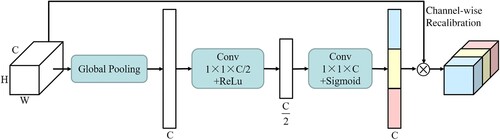
During image segmentation, not all regions in the image contribute equally to the task. The attention model finds the part that contributes the most to the task. Depending on the activation region, the attention mechanism includes spatial attention and channel attention. A difficulty in glacier studies is that some backgrounds have a high spectral similarity to glaciers and can easily be misidentified. The channel attention mechanism focuses on meaningful input feature maps by estimating the contribution of different feature channels to glacier classification and enhancing or suppressing different channels depending on the contribution. The channel-attention model can assign different weights to different feature maps. Feature channels with high contribution to feature classification are weighted high and those with low contribution are weighted low, thus reducing the background misclassification rate.

In this paper, we use the channel squeeze and excitation (cSE) model (Roy, Navab, and Wachinger 2018). As shown in Figure 3, the specific implementation process of this model is to first change the shape of the low-level feature map from [C, H, W] to [C, 1, 1] using the global average pooling method. Two 1×1 convolutions are then used to obtain a C-dimensional vector. Next, the weights of each channel are obtained using the sigmoid function to weigh each channel of the original feature map.

Figure 3. Channel-attention model structure: channel squeeze and excitation (cSE) block (Roy, Navab, and Wachinger 2018).

3.3. Post-processing

The semantic segmentation network classifies each pixel, so it is easy to generate background noise. In particular, the features of some rocks are similar to debris-covered glaciers, so we optimize the output of the network using CRFs. Each pixel has both a category label and a corresponding observation. Each pixel as a node and the pixel-to-pixel relationship as an edge constitutes a CRF. The one-dimensional potential ${\theta }_i\left(x_i\right)$ is the result of the network prediction, which is transformed from the confidence coefficient $P\left(x_i\right)$ output by the network softmax function: (1) ${\theta }_i\left(x_i\right)=-\log \left(P\right(x_i\left)\right)$(1)

where $x$ is the label of the pixels and $P\left(x_i\right)$ is the confidence level at pixel i calculated by the neural network.

The binary potential ${\theta }_{ij}(x_i,x_j)$ describes the relationship between pixels. It encourages similar pixels to be assigned the same label, while pixels that differ more are assigned different labels. This definition of similarity is related to the pixel value and the actual distance of the pixels, so CRF enables the image to be segmented at the boundaries as much as possible: (2) ${\theta }_{ij}(x_i,x_j)=\mu (x_i,x_j)[w_1\exp (-{\displaystyle \frac{\left|\right|p_i-p_j|{|}^2}{2{\sigma }_{\alpha }^2}-{\displaystyle \frac{\left|\right|I_i-I_j|{|}^2}{2{\sigma }_{\text{β}}^2}+w_2\exp (-{\displaystyle \frac{\left|\right|p_i-p_j|{|}^2}{2{\sigma }_{\gamma }^2}\left)\right)]}}}$(2) (3) $\mu (x_i,x_j)=\{\begin{array}{c}1,if{x}_i\ne x_j\\ 0,if{x}_i=x_j\end{array}$(3)

where p is the position of the pixel and I is the RGB color value of the pixel. The expression uses two Gaussian kernels in the two aspects. The hyper parameters ${\sigma }_{\alpha }^{}$, ${\sigma }_{\text{β}}^{}$, and ${\sigma }_{\gamma }^{}$ control the scale of the Gaussian kernels. The formula makes pixels with similar colors and positions have similar labels.

Combining the unary and binary potentials enables a more comprehensive consideration of the relationship between pixels. CRF considers not only the output of the neural network when classifying a pixel, but also the confidence of the surrounding pixels, especially those with closer pixel values. This yields semantic segmentation results with better edges. The optimized result is shown in Equation 4(4) $E\left(x\right)=\sum _i{\theta }_i\left(x_i\right)+\sum _{ij}{\theta }_{ij}(x_i,x_j)$(4) : (4) $E\left(x\right)=\sum _i{\theta }_i\left(x_i\right)+\sum _{ij}{\theta }_{ij}(x_i,x_j)$(4)

4. Experimental results

The raw Landsat 8 image stripes are large. Due to computer hardware limitations, all data were cropped to 512×512 pixels, yielding 7821 images. About 30% were randomly selected as training samples, for a total of 2584 images, 25% of which were negative samples that did not contain glaciers. The samples contained debris-covered glaciers, mountain shadow occlusion, cloud occlusion, water, and other cases that are prone to false extraction, in order to improve the model's ability to recognize glaciers.

To verify the effectiveness of the U-Net network improvement method for glacier extraction proposed in this paper, all images of the whole study area were tested to obtain the accuracy of glacier extraction. The experiments were conducted using U-Net, GlacierNet by Xie et al. (Xie et al. 2020), and the U-Net with channel-attention model cSE (our method), respectively. The epoch is set to 100. The results are shown in Table 1. Accuracy evaluation is performed using semantic segmentation evaluation metrics such as accuracy, recall, and F1-score. The formulae for calculating the three metrics are shown in Equations 5(5) $accuracy={\displaystyle \frac{TP+TN}{TP+TN+FP+FN}}$(5) –7(7) $F1={\displaystyle \frac{2TP}{2TP+FP+FN}}$(7) : (5) $accuracy={\displaystyle \frac{TP+TN}{TP+TN+FP+FN}}$(5) (6) $recall={\displaystyle \frac{TP}{TP+FN}}$(6) (7) $F1={\displaystyle \frac{2TP}{2TP+FP+FN}}$(7)

Table 1. Accuracy metrics of glacier extraction results obtained using U-Net, GlacierNet, U-Net + cSE, respectively.

	Accuracy	Recall	F1 score
U-Net	0.9756	0.8909	0.8887
GlacierNet	0.9689	0.8012	0.8491
U-Net + cSE (ours)	0.9774	0.8788	0.8946

where TP indicates that the pixel label is glacial and the prediction is also glacial, TN indicates that the pixel label is background and the prediction is also background, FP indicates that the pixel label is background and the prediction is glacial, and FN indicates that the pixel label is glacial and the prediction is background.

From the results, it can be seen that the accuracy of the U-Net with cSE for glacier recognition is 97.74% higher than other methods, but recall is reduced compared to the results obtained by U-Net. Accuracy is the ratio of pixels classified correctly to the total number of pixels. Increasing precision shows more pixels are correctly classified. The recall is the ratio of pixels classified as glaciers to the actual glacier pixels. The channel-attention mechanism will make the network model focus more on the features of the glacier and can reduce false identification of the background (Figure 4). Therefore, the pixels classified as glaciers are reduced and the recall is lower than that of U-Net. However, in terms of accuracy, the overall number of correctly classified pixels still increases. The F1 score is a comprehensive performance indicator that strikes a balance between recall and accuracy. The accuracy index and recall index sometimes appear contradictory, so they need to be considered together with the F1 score. The F1 score of our method is higher than the other methods, which shows that our method can extract mountain glaciers more effectively and accurately.

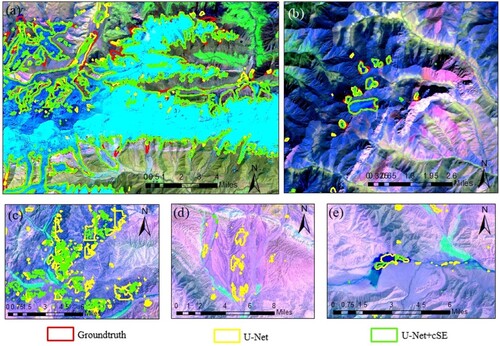
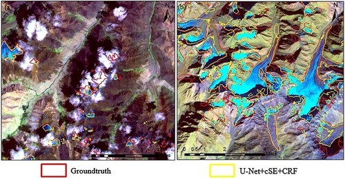
Figure 4. Results of glacier extraction in Ulukchati using U-Net, GlacierNet, U-Net with cSE and after CRF post-processing, respectively.

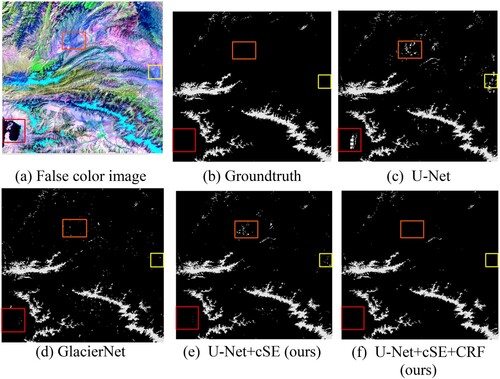
The Ulukchati image in the study area was selected separately for comparison, and the comparison results are shown in Figure 4. Overall, each network model can identify the approximate glacier extent. The glacier boundaries can be identified relatively accurately, both in areas of large and small glacier extent (Figure 5(a) and (b)). However, the U-Net model results in more background misidentifications, especially in water (Figure 4(a), red box) and rocky areas with a similar color to the glacier (Figure 4(a), yellow box). After adding the channel-attention cSE, background misidentification is significantly reduced. For backgrounds with relatively high differences from the glacier features (Figure 5(d)), false recognition can be avoided, and for backgrounds that differ less from glacier features (Figure 5(c) and (e)), the number of falsely identified pixels is reduced. The area of noise is smaller and also more favorable to eliminate noise with post-processing. Therefore, compared to U-Net and GlacierNet, U-Net with channel-attention cSE can extract glacier regions more accurately.

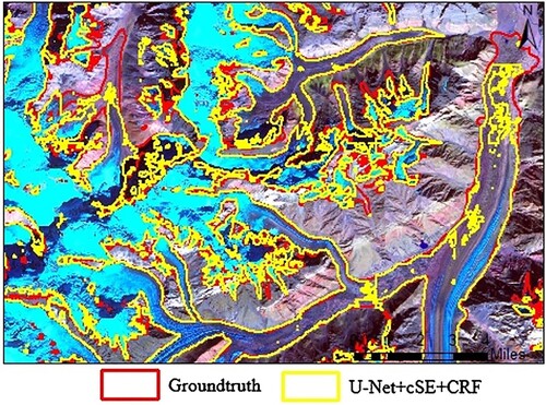
Figure 5. Glacier boundaries in the partial area of the Ulukchati image obtained using U-Net and U-Net with the channel-attention cSE model, respectively.

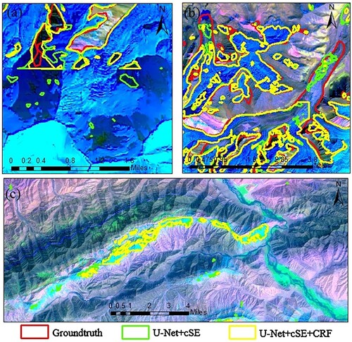
As can be seen in Figure 5, there is still background noise in our results. In this study, the CRF model was used to fine-tune the segmentation results for noise removal and glacier region gap filling. The CRF model requires setting the number of iterations. In natural image recognition, this parameter is generally set to 10 (DeepLab). However, in this study, the accuracy did not increase significantly when the number of iterations was 10 (Table 2). Different parameters were set separately for each image post-processing to determine a better number of iterations. We found that the optimal number of iterations was different in various cases. Taking the Kudara image (less noise, Figure 6) and the Ulukchati image (more noise, Figure 4) as examples, the accuracy is shown in Table 3 by setting 1, 2, 5, and 10 iterations, respectively.

Figure 6. Results of glacier extraction in Kudara using U-Net with cSE.

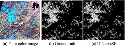
Table 2. Evaluation of glacier extraction accuracy for three cases: no post-processing, CRF iteration of 10, and different iterations for different cases (more noise, iteration of 10; less noise, iteration of 1).

	Accuracy	Recall	F1 score
U-Net + cSE	0.9774	0.8788	0.8946
U-Net + cSE + CRF (iteration 10)	0.9778	0.8646	0.8948
U-Net + cSE + CRF (more noise, iteration 10; less noise, iteration 1)	0.9782	0.8719	0.8976

Table 3. Accuracy of glacier extraction with different iterations.

Iteration	Kudara			Ulukchati
	Accuracy	Recall	F1 score	Accuracy	Recall	F1 score
No post-processing	0.9643	0.8705	0.9033	0.9858	0.8671	0.8967
1	0.9651	0.8659	0.9047	0.9868	0.8635	0.9030
2	0.9649	0.8632	0.9039	0.9870	0.8615	0.9043
5	0.9643	0.8594	0.9022	0.9871	0.8590	0.9049
10	0.9640	0.8573	0.9012	0.9872	0.8577	0.9050

As shown in Table 3, for images with little noise like Kudara, the accuracy gradually decreases as the number of iterations increases. The accuracy is highest when the iteration is 1, and for images with a lot of noise, such as Ulukchati, the accuracy gradually increases with an increase in number of iterations. The accuracy is highest when the number of iterations is 10. CRF makes it easier for pixels with similar colors and adjacent positions to have the same classification. A debris-covered glacier is similar in color to the surrounding rock or earth. During post-processing, debris-covered glaciers may be classified as background and thus underestimated. That is the reason for the recall reduction. On images with less noise, the number of debris-covered glaciers eliminated is greater than the number of backgrounds eliminated as the number of iterations increases. Conversely, for images with more noise, the number of misidentified backgrounds is higher and the number of eliminated backgrounds is greater than eliminated debris-covered glaciers.

For the problem that the optimal iteration varies in different cases, we divided the images into two categories. The iteration was set to 1 for images with less noise and 10 for images with more noise. The high and low noise images were subjectively and artificially judged based on the recognition result with the input image. The final accuracy is shown in Table 2. Both precision and F1 score were improved. The accuracy of glacier extraction for the whole study area reached 97.82%. As an example, the misidentification of the background was significantly reduced after post-processing using CRF for the Ulukchati image (Figure 4(f)). CRF can also fill some holes in specific details (Figure 7(a)). However, there are cases of misidentification of background as debris-covered glaciers (Figure 7(b)). In addition, the CRF method cannot effectively eliminate background with large misidentification ranges and high spectral similarity to the glacier (Figure 7(c)).

Figure 7. Comparison of glacier boundaries before and after post-processing using CRF.

5. Discussion

Compared with U-Net and GlacierNet, our proposed channel-attention U-Net can better distinguish glacier from non-glacier by learning the most discriminative spectral information in the image. From the results, the background misidentification is significantly resolved and glacier extraction is more accurate. The CRF model is also added for post-processing, which reduces background noise, but the method still has some limitations.

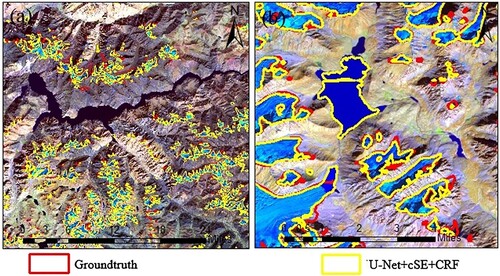
First, it is impossible to completely ensure that other geological features with high spectral similarity to glaciers are not misidentified as glaciers. Bodies of water are especially difficult to distinguish from glaciers. In this study, most of the lakes and rivers could be effectively distinguished from glaciers (Figure 4, Figure 6 and Figure 8(a)). However, a few frozen water bodies are very similar to glaciers and were still misidentified (Figure 8(b)).

Figure 8. Results of image glacier extraction containing water in the Kudara image.

Second, clouds and their shadows and terrain-cast shadows are issues that have historically affected optical remote sensing-based glacier mapping. Our method cannot identify glaciers covered by clouds (Figure 9(a)). It was necessary to select images with as little cloud cover as possible for the study. In cloud-shaded and alpine shadow-covered clean glaciers (Figure 9), although the illumination is relatively low, the gradient is still present to support network classification so it can still be effectively identified, but the debris-covered glaciers in the shadowed area (lower right corner of Figure 9(b)) are underestimated.

Figure 9. Cloud and shadow samples: (a) cloud-covered area; (b) mountain shadow area.

Glaciers consist of clean glaciers and debris-covered glaciers. Debris-covered glaciers are a challenge to study because of their high similarity to the surrounding rocks. Our method can effectively identify clean glaciers and debris-covered glaciers; meanwhile, the misidentification rate of the background is low. However, debris-covered glaciers were still underestimated (Figure 10). Since the two types of glaciers have some spectral differences, in the future we will consider two different methods to identify the two separately in order to improve glacier extraction accuracy.

Figure 10. Extraction results of debris-covered glaciers.

For water, shadows and debris-covered glaciers, our model can still effectively identify most of the area, but this part is underestimated compared to groundtruth.

6. Conclusion

In this study, we proposed a channel-attention U-Net, which adds a channel-attention cSE model to U-Net, and fine-tuned the extraction results using the CRF model to achieve a depiction of mountain glaciers. The method was tested on the Pamir Plateau using Landsat 8 and a DEM as data sources. Compared with U-Net and GlacierNet, our method can extract more accurate glacier regions with a lower misidentification rate for the background. The results show that the channel-attention mechanism can effectively improve the recognition of spectral feature differences between glaciers and non-glaciers by assigning different weights to different feature maps, thus improving the glacier extraction accuracy. In future work, we will consider incorporating the channel-attention model into other semantic segmentation networks to further improve glacier extraction accuracy.

In addition, we also investigated the effect of the number of iterations in the CRF model on glacier recognition. It was found that, when there is little background misidentification, 1 iteration has the highest accuracy; when there are many background misidentifications, 10 iterations have the highest accuracy. Thus, for different images, different iteration numbers should be set. Our results show that CRF as post-processing can indeed effectively improve glacier extraction accuracy. Unfortunately, it hinders the full automation of the whole model. In the future, we will consider adding the CRF model to the last part of the network model to automatically select the number of iterations.

In our subsequent glacier classification study, more data sources should be used, and the inclusion of remote sensing synthetic aperture radar (SAR) images to provide richer features should be considered. In future work, the network model should be further improved to solve the problem that of underestimated debris-covered glaciers. In addition, Zhang et al. (Zhang et al. 2021) showed that DeepLabv3+ has higher accuracy when delineating Greenland glacier calving fronts using U-Net and DeepLabv3+, respectively. Therefore, the extraction of glaciers using models such as DeepLabv3+ will be attempted in the future.

Acknowledgements

We thank the National Aeronautics and Space Administration (NASA) and the United States Geological Survey (USGS) for providing the Landsat-8 data and National Imagery and Mapping Agency (NIMA) for providing the SRTM DEM data. We thank the editors and the reviewers for their valuable comments and suggestions.

Disclosure statement

No potential conflict of interest was reported by the author(s).

Data availability

Pamir Plateau Glacier Range data products are available for free from https://6084/m9.figshare.16778587.

Additional information

Funding

This work was supported in part by the National Natural Science Foundation of China (No.41925007) and the National Natural Science Foundation of China (No. U1711266).

References

- Abdollahi, Abolfazl, Biswajeet Pradhan, and Abdullah M Alamri. 2020. “An Ensemble Architecture of Deep Convolutional Segnet and Unet Networks for Building Semantic Segmentation from High-Resolution Aerial Images.” Geocarto International, 1–16.
- Badrinarayanan, Vijay, Alex Kendall, and Roberto Cipolla. 2017. “Segnet: A Deep Convolutional Encoder-Decoder Architecture for Image Segmentation.” IEEE Transactions on Pattern Analysis and Machine Intelligence 39 (12): 2481–2495.
- Baumhoer, Celia A, Andreas J Dietz, Christof Kneisel, and Claudia Kuenzer. 2019. “Automated Extraction of Antarctic Glacier and ice Shelf Fronts from Sentinel-1 Imagery Using Deep Learning.” Remote Sensing 11 (21): 2529.
- Bishop, Michael P, Radoslav Bonk, Ulrich Kamp Jr, and John F Shroder Jr. Terrain Analysis and Data Modeling for Alpine Glacier Mapping Polar Geography 25 (3):182-201.
- Bolch, Tobias, Brian Menounos, and Roger Wheate. 2010. “Landsat-based Inventory of Glaciers in Western Canada, 1985–2005.” Remote Sensing of Environment 114 (1): 127–137.
- Burns, Patrick, and Anne Nolin. 2014. “Using Atmospherically-Corrected Landsat Imagery to Measure Glacier Area Change in the Cordillera Blanca, Peru from 1987 to 2010.” Remote Sensing of Environment 140: 165–178.
- Chen, Liang-Chieh, George Papandreou, Iasonas Kokkinos, Kevin Murphy, and Alan L Yuille. 2018. “Deeplab: Semantic Image Segmentation with Deep Convolutional Nets, Atrous Convolution, and Fully Connected Crfs.” IEEE Transactions on Pattern Analysis and Machine Intelligence 40 (4): 834–848.
- Cheng, Gong, Junwei Han, and Xiaoqiang Lu. 2017. “Remote Sensing Image Scene Classification: Benchmark and State of the art.” Proceedings of the IEEE 105 (10): 1865–1883.
- Cheng, Daniel, Wayne Hayes, Eric Larour, Yara Mohajerani, Michael Wood, Isabella Velicogna, and Eric Rignot. 2021. “Calving Front Machine (CALFIN): Glacial Termini Dataset and Automated Deep Learning Extraction Method for Greenland, 1972–2019.” The Cryosphere 15 (3): 1663–1675.
- Chhor, Guillaume, Cristian Bartolome Aramburu, and Ianis Bougdal-Lambert. 2017. “Satellite image segmentation for building detection using U-net.” Web: http://cs229.stanford.edu/proj2017/final-reports/5243715.pdf.
- Gardelle, Julie, Etienne Berthier, Yves Arnaud, and Andreas Kääb. 2013. “Region-wide Glacier Mass Balances Over the Pamir-Karakoram-Himalaya During 1999–2011.” The Cryosphere 7 (4): 1263–1286.
- Gardner, Alex S, Geir Moholdt, J. Graham Cogley, Bert Wouters, Anthony A Arendt, John Wahr, Etienne Berthier, Regine Hock, W. Tad Pfeffer, and Georg Kaser. 2013. “A Reconciled Estimate of Glacier Contributions to sea Level Rise: 2003 to 2009.” Science 340 (6134): 852–857.
- Gjermundsen, E. F., R. Mathieu, Andreas Kääb, T. Chinn, B. Fitzharris, and J. O. Hagen. 2011. “Assessment of Multispectral Glacier Mapping Methods and Derivation of Glacier Area Changes, 1978–2002, in the Central Southern Alps, New Zealand, from ASTER Satellite Data, Field Survey and Existing Inventory Data.” Journal of Glaciology 57 (204): 667–683.
- He, Q, Z Zhang, G Ma, and J Wu. 2020. “GLACIER IDENTIFICATION FROM LANDSAT8 OLI IMAGERY USING DEEP U-NET.” ISPRS Annals of Photogrammetry, Remote Sensing & Spatial Information Sciences 5 (3).
- Huang, Zhongling, Zongxu Pan, and Bin Lei. 2020. “What, Where, and how to Transfer in SAR Target Recognition Based on Deep CNNs.” Ieee Transactions on Geoscience and Remote Sensing 58 (4): 2324–2336.
- Jamil, Akhtar, Aftab Ahmad Khan, Bulent Bayram, Javed Iqbal, Gomal Amin, Mirsat Yesiltepe, and Dostdar Hussain. 2019. Spatio-Temporal Glacier Change Detection Using Deep Learning: A Case Study Of Shishper Glacier In Hunza. Paper presented at the International Symposium on Applied Geoinformatics.
- Karimi, Neamat, Morteza Eftekhari, Manuchehr Farajzadeh, Soodabeh Namdari, Ali Moridnejad, and Danesh Karimi. 2015. “Use of Multitemporal Satellite Images to Find Some Evidence for Glacier Changes in the Haft-Khan Glacier, Iran.” Arabian Journal of Geosciences 8 (8): 5879–5896.
- Mohajerani, Yara, Michael Wood, Isabella Velicogna, and Eric Rignot. 2019. “Detection of Glacier Calving Margins with Convolutional Neural Networks: A Case Study.” Remote Sensing 11 (1): 74.
- Mölg, Nico, Tobias Bolch, Philipp Rastner, Tazio Strozzi, and Frank Paul. 2018. “A Consistent Glacier Inventory for Karakoram and Pamir Derived from Landsat Data: Distribution of Debris Cover and Mapping Challenges.” Earth System Science Data 10 (4): 1807–1827.
- Nie, Yong, Qiao Liu, and Shiyin Liu. 2013. “Glacial Lake Expansion in the Central Himalayas by Landsat Images, 1990–2010.” Plos One 8 (12): e83973.
- Nijhawan, Rahul, Josodhir Das, and Raman Balasubramanian. 2018. “A Hybrid CNN + Random Forest Approach to Delineate Debris Covered Glaciers Using Deep Features.” Journal of the Indian Society of Remote Sensing 46 (6): 981–989.
- Paul, Frank. 2002. “Changes in Glacier Area in Tyrol, Austria, Between 1969 and 1992 Derived from Landsat 5 Thematic Mapper and Austrian Glacier Inventory Data.” International Journal of Remote Sensing 23 (4): 787–799.
- Paul, Frank, Tobias Bolch, Andreas Kääb, Thomas Nagler, Christopher Nuth, Killian Scharrer, Andrew Shepherd, Tazio Strozzi, Francesca Ticconi, and Rakesh Bhambri. 2015. “The Glaciers Climate Change Initiative: Methods for Creating Glacier Area, Elevation Change and Velocity Products.” Remote Sensing of Environment 162: 408–426.
- Paul, Frank, Solveig H Winsvold, Andreas Kääb, Thomas Nagler, and Gabriele Schwaizer. 2016. “Glacier Remote Sensing Using Sentinel-2. Part II: Mapping Glacier Extents and Surface Facies, and Comparison to Landsat 8.” Remote Sensing 8 (7): 575.
- Pope, Allen, and W. Gareth Rees. 2014. “Impact of Spatial, Spectral, and Radiometric Properties of Multispectral Imagers on Glacier Surface Classification.” Remote Sensing of Environment 141: 1–13.
- Raper, Sarah CB, and Roger J Braithwaite. 2006. “Low sea Level Rise Projections from Mountain Glaciers and Icecaps Under Global Warming.” Nature 439 (7074): 311–313.
- Raup, Bruce H, Liss M Andreassen, Tobias Bolch, and Suzanne Bevan. 2015. “Remote Sensing of Glaciers.” Remote Sensing of the Cryosphere, 123–156.
- Raup, Bruce, Andreas Kääb, Jeffrey S Kargel, Michael P Bishop, Gordon Hamilton, Ella Lee, Frank Paul, Frank Rau, Deborah Soltesz, and Siri Jodha Singh Khalsa. 2007. “Remote sensing and GIS technology in the Global Land Ice Measurements from Space (GLIMS) project.” Computers & Geosciences 33 (1):104-125.
- Raup, Bruce, Adina Racoviteanu, Siri Jodha Singh Khalsa, Christopher Helm, Richard Armstrong, and Yves Arnaud. 2007. “The GLIMS geospatial glacier database: a new tool for studying glacier change.” Global and Planetary Change 56 (1-2):101-110.
- Robson, Benjamin Aubrey, Tobias Bolch, Shelley MacDonell, Daniel Hölbling, Philipp Rastner, and Nicole Schaffer. 2020. “Automated Detection of Rock Glaciers Using Deep Learning and Object-Based Image Analysis.” Remote Sensing of Environment 250: 112033.
- Ronneberger, Olaf, Philipp Fischer, and Thomas Brox. 2015. U-net: Convolutional networks for biomedical image segmentation. Paper presented at the International Conference on Medical image computing and computer-assisted intervention.
- Roy, Abhijit Guha, Nassir Navab, and Christian Wachinger. 2018. Concurrent spatial and channel ‘squeeze & excitation’in fully convolutional networks. Paper presented at the International conference on medical image computing and computer-assisted intervention.
- Salomonson, Vincent V, and Igor Appel. 2006. “Development of the Aqua MODIS NDSI Fractional Snow Cover Algorithm and Validation Results.” Ieee Transactions on Geoscience and Remote Sensing 44 (7): 1747–1756.
- Singh, Dhanendra K, Praveen K Thakur, Bhanu Prasad Naithani, and Suvrat Kaushik. 2021. “Quantifying the Sensitivity of Band Ratio Methods for Clean Glacier ice Mapping.” Spatial Information Research 29 (3): 281–295.
- Sofla, Reza Akbari Dotappeh, Tayeb Alipour-Fard, and Hossein Arefi. 2021. “Road Extraction from Satellite and Aerial Image Using SE-Unet.” Journal of Applied Remote Sensing 15 (1): 014512.
- Van Zyl, Jakob J. 2001. “The Shuttle Radar Topography Mission (SRTM): A Breakthrough in Remote Sensing of Topography.” Acta Astronautica 48 (5-12): 559–565.
- Wang, Guang, Yue Liu, Huifang Shen, Shudong Zhou, Jinzhou Liu, Hegao Sun, and Yan Tao. 2020. Glacier Area Monitoring Based on Deep Learning and Multi-sources Data. Paper presented at the International Conference on Computer Engineering and Networks.
- Wang, Shengjie, Mingjun Zhang, Zhongqin Li, Feiteng Wang, Huilin Li, Yaju Li, and Xiaoyan Huang. 2011. “Glacier Area Variation and Climate Change in the Chinese Tianshan Mountains Since 1960.” Journal of Geographical Sciences 21 (2): 263–273.
- Xie, Zhiyuan, Umesh K. Haritashya, Vijayan K. Asari, Brennan W. Young, Michael P. Bishop, and Jeffrey S. Kargel. 2020. “GlacierNet: A Deep-Learning Approach for Debris-Covered Glacier Mapping.” IEEE Access 8: 83495–83510.
- Zemp, Michael, Holger Frey, Isabelle Gärtner-Roer, Samuel U Nussbaumer, Martin Hoelzle, Frank Paul, Wilfried Haeberli, Florian Denzinger, Andreas P Ahlstrøm, and Brian Anderson. 2015. “Historically Unprecedented Global Glacier Decline in the Early 21st Century.” Journal of Glaciology 61 (228): 745–762.
- Zhang, Enze, Lin Liu, and Lingcao Huang. 2019. “Automatically Delineating the Calving Front of Jakobshavn Isbræ from Multitemporal TerraSAR-X Images: A Deep Learning Approach.” The Cryosphere 13 (6): 1729–1741.
- Zhang, Enze, Lin Liu, Lingcao Huang, and Ka Shing Ng. 2021. “An Automated, Generalized, Deep-Learning-Based Method for Delineating the Calving Fronts of Greenland Glaciers from Multi-Sensor Remote Sensing Imagery.” Remote Sensing of Environment 254: 112265.
- Zhang, Liangpei, Lefei Zhang, and Bo Du. 2016. “Deep Learning for Remote Sensing Data: A Technical Tutorial on the State of the art.” IEEE Geoscience and Remote Sensing Magazine 4 (2): 22–40.