Quantitative prediction and evaluation of geothermal resource areas in the southwest section of the Mid-Spine Belt of Beautiful China

ABSTRACT

The geothermal resources in the southwest section of the Mid-Spine Belt of Beautiful China are abundant, but the quantitative prediction and evaluation of geothermal resources are very difficult. Based on geographic information system (GIS) and remote sensing (RS) platforms, six impact factors, namely land surface temperature, fault density, Gutenberg–Liszt B value, formation combination entropy, distance to river and aeromagnetic anomaly were selected. Through the establishment of the certainty factor model (CF), weights of the information entropy certainty factor model (ICF) and weights of the evidence certainty factor model (ECF), the geothermal potential in the study area were predicted quantitatively. Based on the ECF results, the six main geothermal resource areas were delineated. The results show that (1) ECF had high prediction accuracy (success index is 0.00405%, area ratio is 0.867); (2) The geothermal resource areas obtained were Ganzi–Ya’an–Liangshan, Panzhihua–Liangshan, Dali–Chuxiong, Nujiang–Baoshan, Diqing–Dali, and Lijiang–Diqing. The results provide a basis for the effective development and utilization of geothermal resources in the southwest section of the mid-ridge belt.

KEYWORDS:

• Mid-Spine Belt of Beautiful China
• certainty factor
• geothermal resource area
• weights of evidence

1. Introduction

Geothermal resources are valuable and comprehensive resources with the advantages of wide distribution, large reserves, eco-friendliness, low carbon emissions and high utilization coefficient (Zhou, Liu, and Liu 2015). It is of great practical significance to carry out geothermal power generation project construction and industrial development planning in regions rich in geothermal resources to improve energy structure, boost the local economy, promote sustainable development and achieve carbon peak and carbon neutral goals. The ‘Mid-Spine Belt of Beautiful China’(MSBBC) is the strategic need for new land space planning with high-quality development in the modern era and is a strategic move to reduce the imbalance of development between the east and the west (Wang et al. 2021). The MSBBC spans different natural zones and has a rich and diverse natural ecological environment. The southwest section of the MSBBC is located in the Himalayas. However, due to the challenges of exploration and development, a large number of geothermal resources in this region have not been exploited or utilized, and the model of geothermal resource exploration and evaluation is too simple, such that the exploration work cannot serve the construction of geothermal engineering (Wang et al. 2020). Therefore, it is particularly important to establish an automatic prediction model based on remote sensing data and a GIS platform to quantitatively predict the geothermal resource potential of key areas of China, especially in the southwest section of the MSBBC.

In the study of predicting geothermal resource potential, the common methods include geophysical exploration, drilling and geochemical methods (Watson, Kruse, and Hummer 1990; Yan et al. 2019). These methods are limited in some basic issues, such as long cycles, large capital investment, and extensive engineering requirements (Yan et al. 2017). Therefore, it is necessary to construct a scientific and accurate multi-factor prediction model to improve the automation degree and demarcation accuracy of geothermal potential prediction (Zhao et al. 2021). Remote sensing can be used to evaluate surface heat losses, and to recognize suitable hot-spring sites using the thermal bands (Abdel-Fattah, Shendi, and Kaiser 2020). Enhanced Thematic Mapper (ETM+7), Operational Land Imager (OLI-8) and TIRS Landsat satellite images have been recently employed to estimate Land Surface Temperature (LST), and to indicate geothermal potentiality (Yuliang and Yongming 2008; Cristóbal et al. 2018; El Bouazouli et al. 2019). The evaluation and prediction method based on GIS platform has been widely used in metallogenic prediction and evaluation, groundwater resources evaluation and prediction, collapse, landslide, fire risk evaluation, pollution risk evaluation and other fields (Chen et al. 2017; Hou 2013; Fan et al. 2012). For example, the Bayesian statistical model was used in the Gulf of Suez coastal area in Egypt to find potential geothermal areas. (Abuzied, Kaiser, and Shendi 2020); The geothermal anomaly area was quantitatively predicted and delineated along the Sichuan–Tibet Railway in southwest China by using the index coverage, entropy weight and evidence weight information model (Zhao et al. 2021). Therefore, it is feasible to achieve quantitative prediction of geothermal resource potential areas by evaluating the influencing factors closely related to geothermal distribution.

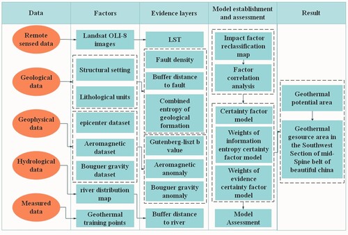
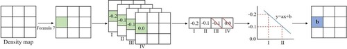
At present, however, the evaluation and prediction methods based on GIS platforms mostly adopt the information value method and the weight-of-evidence method. The certainty factor method is used to analyze the sensitivity of factors affecting the occurrence of an event. It analyzes the choice of multiple applications of impact factors through their sensitivity. It can effectively address the problems of many influencing factors and the different sensitivity of each factor (Li and Zhang 2018). However, the application of geothermal resource potential prediction and evaluation is rarely seen, and the research on the weighted certainty factor model is not sufficient. In this study, the spatial relationship between the distribution of geothermal training sites and surrounding control factors was quantified, and a model for quantitative prediction and evaluation of geothermal potential areas was built (Johnson 2014; Mcguire et al. 2015; Crespo et al. 2013). It was possible to predict the geothermal potential areas in the southwest section of the MSBBC, and delineate the geothermal resource areas, providing suggestions and decision-making support for balanced regional development and the realization of carbon peaking and carbon neutrality goals. The technology and methodology flow chart of this paper is shown in Figure 1.

Figure 1. The technology and methodology flow chart of this study.

2. Study area

The MSBBC is a regional space from northeast to southwest proposed to be delimited in consideration of the new development needs of China's strategy in the future. On the Chinese map, this area is located in the ‘middle ridge’ (Figure 2). This area is a cluster of relatively poor areas in China, an ecological protection belt, and a space safety belt. According to the differences of nature, society, economy and culture, the ‘middle ridge belt’ is divided into three sections: Northeast section (I) Heilongjiang and Xing’an Eco-tourism Economic Belt; Middle section (II) Erdos–Hohhot–Zhangjiakou–Datong–Xilin Gol Eco-economic and Cultural Zone and Xi’an–Lanzhou–Yinchuan–Taiyuan Eco-economic and Cultural Zone; Southwest Section (III) Chongqing–Chengdu–Kunming–Ruili Ecological economic Belt cultural Zone (Wang et al. 2020).

Figure 2. Factor distribution and geographical location of the study area.

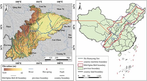
The study area is located in southwest China, extends between latitudes 22° 36’ to 34 ° 46’ N and longitudes 97°38’ to111° 8’ E with a total area 619026 km², covering the southwest section (III) of the MSBBC, including the eastern part of Sichuan Province, the northern part of Yunnan Province and the western part of Chongqing(Figure 2). The terrain mainly consists of basins and plateaus, of which the elevation of the Sichuan Basin is about 500 m, the elevation of the Yunnan Plateau is about 2000m, and the elevation of the eastern margin of the Qinghai–Tibet Plateau is basically above 3500 m (Cao et al. 2011). The gorge area is mainly distributed in the Hengduan Mountains and is mainly caused by the long-term drastic cutting action of several major rivers such as the Lancang, Jinsha and Nu Rivers, so it shows significant surface cutting and undulation. The climate in the study area is humid. Due to the uplift of the Qinghai Tibet Plateau, the temperature and precipitation in this area are very different. The average annual temperature in the East is 24°C, and the lowest average annual temperature in the west is below 0°C. The precipitation varies by thousands of millimeters from southeast to northwest, and the temporal and spatial distribution is extremely uneven.

The study area is located in the eastern part of the global latitudinal Tethyan orogenic system, which is a complex tectonic domain formed by arc–arc and arc-continent collision between the southwest margin of the Pan-Cathaysia continent and the northern margin of the southern Gondwana continent and then by shrinking of the small ocean basin (Liu et al. 2010). There are many lithology layers in the interior of the region, complicated geological conditions, dense fracture development, frequent seismic activity and intense geothermal activity. Due to the collision between the Indian plate and the Eurasian plate, strong compressive deformation is formed in this area, resulting in complex fault structures and strike-slip structures. Under these geological conditions, a large number of hot springs and geothermal areas are formed and distributed in a belt along the fault zone. The geothermal resources in the study area are mainly controlled by fault structures, especially the Cenozoic fault structures, which provide good channels for hydrothermal activities and form obvious banded geothermal resources. The hot water supply sources in the area are mainly atmospheric precipitation, ice and snow melt water and surface water infiltration. Their water infiltrates to the deep along the fault or contact zone of different rock masses and rises to the shallow along the channel after being heated by the surrounding rock. The negative gravity anomaly is formed by frequent earthquakes and volcanic activities in the region and the material loss caused by the overflow of volcanic eruption magmatic material. The residual magnetism was obtained during the cooling process after the overflow of hot magma, but the magnetic irregularity is caused by multiple eruptions (Zhou Xiang, and Deng 1997; Jiang, Tan, and Zhang 2012). Therefore, quantitative prediction and evaluation of geothermal resource potential in this region has very important application value.

3. Data and methods

Combined with the geological, geophysical, hydrological and other data in the overview of the study area. The spatial data were selected rationally to develop the certainty factor model (CF) and to derive eight evidence layers involving LST, fault density, buffer distance to fault, combined entropy of geological formation, Gutenberg–Liszt b value, aeromagnetic anomaly, Bouguer gravity anomaly and buffer distance to the river.

The spatial data used in this study were divided into target data and exploration data. The target data include Landsat-8 satellite data, fault data (Figure 2), lithology data, epicenter data, a river distribution map (Figure 2), aeromagnetic data and Bouguer gravity anomaly data, and the exploration data are geothermal training site data. Hotspot data were obtained from the geological cloud of the China Geological Survey (https://geocloud.cgs.gov.cn/) and the field survey (Figure 2) and Landsat-8 satellite data from the United States Geological Survey (https://earthexplorer.usgs.gov/). The fault data, epicenter data and lithology data were obtained from the Geological cloud of the China Geological Survey (https://geocloud.cgs.gov.cn/).

3.1. Spatial datasets

3.1.1. Geothermal training points

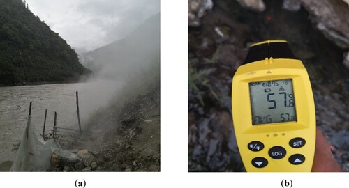
The hot springs in the southwest section of the MSBBC are widespread and have significant differences in heat flow. High-temperature hot springs and geothermal Wells are probably distributed together and may belong to the same geothermal system in an area of 10 km² (Hedlund, Cole, and Williams 2012). The hot springs exposed on the surface imply the existence of high-temperature geothermal phenomena. In the calculation of the prediction model, hot springs and adjacent areas can be specified as known geothermal training sites. The data of geothermal training sites in the research area come from the Geological cloud of the China Geological Survey and field investigation (Figure 3). According to statistics, 211 selected geothermal training points were selected (Figure 2).

Figure 3. Hot spring surrounding environment and measurement: (a) Surrounding environment of a hot spring; (b) Measurement of a hot spring.

3.1.2. Land surface temperature

The land surface temperature (LST) inversion can extract heat information successfully (Vlassova et al. 2014), providing an provide objective basis for the determination of the geothermal anomaly, and remote sensing image information processed by the LST has been successfully used in the study of geothermal resources and disaster investigation (Zhang and Zhang 2006). LST mainly comes from the action and influence of geological activities and solar radiation. One effective way to establish LST is thermal infrared remote sensing. Landsat-8 image data have many advantages: data can be downloaded directly from the U.S. Geological Survey website, and the Thermal infrared band 10 has a spatial resolution of 100 m, which can effectively obtain fine thermal field scenes and LST anomalies.

There are many algorithms for LST inversion through landsat-8 remote sensing images (Wang et al. 2001; Wan and Li 1997; Sobrino, Jiménez-Muñoz, and Paolini 2004; Jiménez-Muñoz and Sobrino 2003; Becker and Li 1990). According to the surface heat radiation conduction equation, Qin Zhihao et al. derived the mono-window algorithm through a series of simplified methods (Qin, Zhang, and Arnon 2001), and the formula can be expressed as: (1) $T_s=\{a(1-C_i-D_i)+[b(1-C_i-D_i)+C_i+D_i]T_b-D_i{T}_a\}/C_i$(1) (2) $C_i={\epsilon }_i{\tau }_i$(2) (3) $D_i=(1-{\tau }_i)[1+{\tau }_i(1-{\epsilon }_i)],$(3) where T_s is the retrieved LST; T_b is the brightness temperature (k) obtained by the sensor; T_a is the average atmospheric temperature (k); a and b are the linear regression coefficients, which are associated with the temperature range of the study area; C and D are intermediate variables; ϵ is the surface emissivity; and τ is the atmospheric transmittance (Jin and Gong 2018).

The main aspect of the terrain correction method is statistics; it is assumed that there is a certain linear relationship between. Regression analysis is used to establish the image pixels and radiation brightness values of the linear relationship between solar radiation and expression, then according to the regression relationship the received radiation energy slope is corrected to the horizontal position, eventually eliminating topographic influence. The formula can be represented as: (4) $\cos (i)=\cos (z)\cos (S)+\sin (z)\sin (S)\cos ({\mathrm{\Phi }}_x-{\mathrm{\Phi }}_n)$(4) (5) $L_T=m\cos (i)+b,$(5) (6) $\mathrm{LH}=\mathrm{LT}-[m\cos (i)+b]+\overline{L_T},$(6) where i is the effective incidence angle of the sun; z is the solar zenith angle; ${\mathrm{\Phi }}_{\mathrm{x}}$ is the sun azimuth angle; S is the pixel slope angle; ${\mathrm{\Phi }}_{\mathrm{n}}$ is the pixel aspect angle; L_T is the radiance value of the ground object before correction; m and B are the parameters obtained by regression analysis; L_H is the radiance value after correction and L_T is the radiance value of ground features in a flat area.

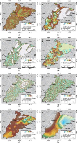
In this study, a total of 180 landsat-8 data images in the winter of 2013–2020 in the study area were obtained, the LST values were obtained by using the mono-window algorithm, terrain correction was carried out and multi-year average LST was calculated (Figure 4(a)) as the input data of the geothermal anomaly prediction model.

Figure 4. Factor maps: (a) LST; (b) Fault density; (c) Buffer distance to fault; (d) Gutenberg–Liszt b value; (e) Combined entropy of geological formation; (f) Buffer distance to river; (g) Aeromagnetic anomaly; (h) Bouguer gravity anomaly.

3.1.3. Fault density

Tectonism is mainly reflected in faults and other macroscopic manifestations, mainly according to the density distribution of various tectonic lines (Liu 2003). The more complex the fracture structure is, the more secondary structural planes in the rock mass, the more broken rock mass and the greater the possibility of geothermal phenomenon. The intensity of structural development can be analyzed using the fault density, and then the fault density map can be obtained (Figure 4(b)).

3.1.4. Buffer distance to fault

The distribution of geothermal anomalies is closely related to fault activity, with deeper faults forming seepage channels that allow groundwater to flow deep into the earth's crust and be heated to high temperatures. Geothermal anomalies can occur when hot water returns to the surface again through shallow faults (Revil and Pezard 1998). Based on the fault data (Figure 2), a fault buffer distance map can be obtained. From the fault buffer distance map (Figure 4(c)), it can be seen that each pixel contains the vertical distance information from the nearest fault, and the hotspots are generally within the distribution range close to the fault.

3.1.5. Gutenberg–Liszt b value

In order to determine the correlation between seismic activity and geothermal system, it is necessary to analyze the characteristics of seismic activity in the study area. In this study, the seismic activity parameter (Gutenberg–Liszt B value) was selected to characterize the characteristics of seismic activity. The B value can reflect the frequency distribution of earthquake magnitude, which is the basic parameter of earthquake hazard and earthquake prediction analysis (Ren 2012). In 1949, Gutenberg and Richter discovered a linear relationship between the frequency of earthquakes and their magnitude. It refers to the statistical relationship between the number of earthquakes n and the earthquake magnitude m within the interval of (m, m + dm) within a certain time range in the research area: (7) $lg{\lambda }_m=a-bm$(7) where m is the earthquake magnitude; λ_m is the annual average frequency of earthquakes with magnitude greater than m. a is the constant related to earthquake incidence; b is the magnitude slope, which represents the ratio of the frequency of earthquakes of different magnitudes.

The study area was divided into 61870137 grids with a size of 100 m × 100 km, and the number of earthquakes occurring within a radius of 10 km was calculated with each grid as the center, and then the annual average number n of earthquakes with magnitude ≥ m was obtained. In order to calculate the B value of each grid, it is essential to count the annual average number of earthquakes with multiple magnitudes (Figure 5). In this study, approximately equally spaced earthquake magnitude segment values were selected: 4–5, 5–6, 6–7, 7–8 and >8. The annual average number of earthquakes of the above five levels can be calculated, and the B values of each grid can be obtained. The Gutenberg-Richter B value diagram (Figure 4(d)) can effectively represent the seismic activity characteristics of a vast area (Ian 1992).

Figure 5. The calculation of the Gutenberg–Liszt b value.

3.1.6. Combined entropy of geological formation

Stratigraphic assemblage entropy is the most basic form of geological anomaly. It refers to the assemblage entropy anomaly of diverse geological bodies or various attributes of the same geological body in unit volume or area, which is calculated from lithologic distribution data (Zhao and Chi 1991; Chi and Zhao 2000). In a specific range, the higher the entropy value, the higher the variation degree of geological structure, and the higher the possibility of geothermal anomalies in this range (Chen et al. 2021). The calculation steps of formation combination entropy are as below (Figure 6):

Figure 6. The calculation of the combined entropy of geological units.

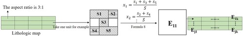
First, the lithology map is divided into grid units, and the long axis direction, size and shape of the units need to be considered. The direction of the long axis should be consistent with the direction of the regional tectonic line. The main fault direction in the study area is southeast, so the long axis is also southeast. The shape of the grid element should correspond to that of the stratum. After the grid element is determined, the independent lithologic area in the element is calculated, and then the sum of the area in the element is calculated, and the ratio of each lithologic area in the element to the area xi (I  = 1,2,3 … , n). Finally, the formation combination entropy is calculated as follows: (8) $E_{jk}=-\sum _{i=1}^n{x}_i\ln x_i/\ln n,$(8) where n is the lithology type existing in the grid unit and j and k are the row number and column number of the unit. The calculated combined entropy of the geological formation is shown in Figure 4(e). The high values for the combination entropy are concentrated in the linear area with sharp changes in lithology, which has a high spatial correlation with the pattern of geological faults.

3.1.7. Buffer distance to river

Under certain geological conditions, when the local groundwater depth is high, it is heated by the surrounding rock and circulates upward, which increases the local temperature of the surrounding rock and forms a shallow geothermal high temperature anomaly (Zhang et al. 2000). Abundant precipitation and numerous rivers in the study area can provide water for geothermal formation. In order to study the spatial relationship between water system and geothermal activity, the river distribution was converted into a distance map to the water system (Figure 4(f)).

3.1.8. Aeromagnetic anomaly

Aeromagnetic anomaly distribution is often used to clearly indicate the area of groundwater thermal activity and the area of tectonic stress changes (Institute of Geography; CAS 2015). An aeromagnetic anomaly map can be used in model construction without special and complicated transformation. Theoretically, low aeromagnetic values are closely related to the distribution of geothermal anomalies. In the active range of groundwater heat, the aeromagnetic properties of rocks are weakened due to thermal alteration. In addition, the aeromagnetic properties of rock distributed along the stress direction will be reduced under the action of tectonic stress, so the aeromagnetic properties of rock will also be weakened in the tectonic fracture zone (Aydogan 2011). The Aeromagnetic Anomaly map generated is shown in Figure 4(g).

3.1.9. Bouguer gravity anomaly

The Bouguer gravity anomaly area refers to the area where the density of crustal material changes sharply along the horizontal direction and is a symbol of the existence of a graben system (Wang 2013). It is caused by the uneven distribution of underground rock mass and mineral density, or the density difference between geological body and surrounding rock. The Bouguer gravity anomaly can linearize large fault structures, and tectonic activity is conducive to the occurrence of geothermal areas. The Bouguer gravity map generated is shown in Figure 4(h).

3.2. Factor reclassification and independence

3.2.1. Factor reclassification

In order to obtain the appropriate classification diagram of impact factors, appropriate threshold values should be adopted. In this study, the natural breakpoint method was adopted to divide each impact factor into seven levels (Table 1). At the same time, when applying the model, the size of grid cells should take into account the scale range of the research area, the similarity of the geological environment of grid cells and the ability for processing the calculation (Tang and Yang 2004). Therefore, all layers were resampled into 100 × 100 m grids after factor classification (Figure 7).

Figure 7. Factor reclassification maps: (a) LST; (b) Fault density; (c) Buffer distance to fault; (d) Gutenberg–Liszt b value; (e) Combined entropy of geological formation; (f) Buffer distance to river; (g) Aeromagnetic anomaly; (h) Bouguer gravity anomaly.

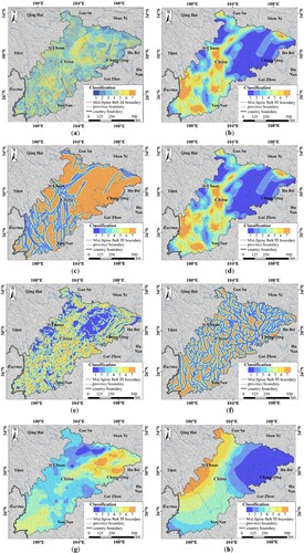
Table 1. Reclassification threshold for impact factor maps.

Impact factors	Class
	1	2	3	4	5	6	7
LST (°C)	−10.00∼−0.57	−0.57∼5.64	5.64∼9.92	9.92∼13.99	13.99∼18.28	18.28∼23.42	23.42∼44.62
Fault density (km/km^2)	0.000∼0.007	0.007∼0.019	0.019∼0.030	0.030∼0.042	0.042∼0.052	0.052∼0.064	0.064∼0.093
Buffer distance to fault (km)	0∼2	2∼4	4∼6	6∼8	8∼10	10∼12	>12
Gutenberg–Liszt b value	−3.89∼−3.00	−3.00∼−2.52	−2.52∼−2.14	−2.14∼−1.86	−1.86∼−1.55	−1.55∼−1.17	−1.17∼0.00
Combined entropy of geological formation	0∼10	10∼20	20∼40	40∼50	50∼60	60∼80	80∼100
Buffer distance to river (km)	0∼2	2∼4	4∼6	6∼8	8∼10	10∼12	>12
Aeromagnetic anomaly (nT)	−250∼−114	−114∼−59	−59∼−22	−22∼16	16∼62	62∼128	128∼310
Bouguer gravity anomaly (mgal)	−440∼−364	−364∼309	−309∼−259	−259∼−213	−213∼−169	−169∼−123	−123∼70

3.2.2. Independence test

The establishment of the model is based on the independence of each input factor of the model. This study tested the independence of each factor by calculating the correlation coefficient according to the result of factor classification. The calculation results are shown in Table 2. When the correlation coefficient between each factor is |R|≤0.3, it can be seen as independent (Zhao and Song 2011; Zhang 2019). It can be seen from the table the Bouguer gravity anomaly is highly correlated with the aeromagnetic anomaly, and fault density is highly correlated with distance to fault. Therefore, the Bouguer gravity anomaly and buffer distance to fault were excluded in this study.

Table 2. Correlation of impact factor maps.

Impact factors	LST	Fault density	Buffer distance to fault	Gutenberg–Liszt b value	Combined entropy	Buffer distance to River	Aeromagnetic anomaly	Bouguer gravity anomaly
LST	1.000	0.055	−0.079	0.043	0.041	−0.161	−0.031	0.153
Fault density	0.055	1.000	−0.781	0.038	0.124	−0.157	0.191	−0.021
Buffer distance to fault	−0.079	−0.781	1.000	−0.061	−0.147	0.165	−0.179	−0.041
Gutenberg–Liszt b value	0.043	0.038	−0.061	1.000	0.050	−0.054	−0.136	0.121
Combined entropy	0.041	0.124	−0.147	0.050	1.000	−0.060	0.063	0.089
Buffer distance to river	−0.161	−0.157	0.165	−0.054	−0.060	1.000	0.029	−0.075
Aeromagnetic anomaly	−0.031	0.191	−0.179	−0.136	0.063	0.029	1.000	−0.398
Bouguer gravity anomaly	0.153	−0.021	−0.041	0.121	0.089	−0.075	−0.398	1.000

3.3. Model establishment

3.3.1. Certainty factor model

The CF is a probability function which is used to analyze the sensitivity of different factors affecting the occurrence of an event (Shortliffe 1975). The geothermal occurrence is caused by the joint action of many factors. Based on the selected influencing factors, the CF can be used to predict geothermal resources. Its calculation formula is as follows:                            (9)where K_CF is the deterministic coefficient, ranging from −1 to 1. The larger the value, the higher the possibility of geothermal areas in the unit. The calculation results of K_CF are shown in Table 3. P_a is the conditional probability of the existence of geothermal in the grading layer of the influence factor. The ratio of the number of hotspots in the grading layer to the number of grids in the grading layer is presented. P_s is the prior probability of geothermal occurrence. In the research area, the probability of geothermal training points appearing in a random grid cell is the prior probability, and the calculation formula is as follows: (10) $P_s={\displaystyle \frac{N}{T}}$(10) where P_s is the prior probability; N is the number of evaluation units of terrestrial hotspots and T is the total number of evaluation units in the study area. Here the prior probability value is the ratio of the total number of hotspots to the total number of grids in the study area (0.00034%).

3.3.2. Weights of information entropy certainty factor model

The ICF uses information entropy theory to obtain the objective weight of each influencing factor. The information entropy theory was proposed by Shannon. The smaller the entropy value of the influencing factor, the greater the density change of the geothermal hotspot in each classification, the higher the corresponding weight value, and the greater the influence of this factor on the prediction and evaluation of geothermal resources (Shannon and Weaver 1947). The formula for calculating geothermal density is:

Table 3. Values for impact factors.

Impact factors		Class
		1	2	3	4	5	6	7
LST	Points	2	3	21	51	67	39	28
	Grids	2746163	9377565	14178153	14388675	10792587	7363298	3023696
	KCF	−0.935	−0.551	−0.392	0.177	0.649	0.511	0.704
	Wi	1.927
	Ci	3.132
Fault density	Points	27	35	29	28	33	40	19
	Grids	16319841	10342239	7870488	7544999	8261545	7097753	4433272
	KCF	−0.839	−0.443	0.243	0.443	0.611	0.727	0.775
	Wi	1.254
	Ci	3.437
Combined entropy of geological formation	Points	42	12	33	26	32	45	21
	Grids	12833637	4644366	6827867	11139509	9880914	11590714	4953130
	KCF	−0.606	0.271	0.298	0.388	0.541	0.459	0.648
	Wi	0.587
	Ci	2.215
Gutenberg–Liszt b value	Points	1	39	36	68	44	12	11
	Grids	669810	17537021	8411018	19008984	10109056	2660823	3473425
	KCF	−0.104	0.239	0.476	0.331	0.412	0.507	−0.026
	Wi	0.381
	Ci	1.716
Buffer distance to river	Points	82	44	23	16	15	9	22
	Grids	10843262	9814951	8952750	7899275	6723368	5366270	12270261
	KCF	0.771	0.369	0.133	0.027	−0.104	−0.263	−0.583
	Wi	1.552
	Ci	1.394
Aeromagnetic anomaly	Points	4	23	46	67	54	10	7
	Grids	1624662	6002854	20990204	15372369	11610042	4643017	1626989
	KCF	−0.438	0.341	−0.151	−0.027	0.212	0.155	−0.356
	Wi	0.425
	Ci	0.962

(11) $d_{ij}={\displaystyle \frac{N_{ij}}{S_{ij}}i=1,2,\dots ,m;j=1,2,\dots ,n}$(11) where d_ij represents the geothermal incidence rate of the ith and jth grade of the impact factor, m is the number of factors affecting geothermal distribution, and n is the number of grades of each grade of the impact factor.

The formula used to calculate the normalization value for points can be expressed as follows: (12) $K_{ij}={\displaystyle \frac{d_{ij}}{{\sum }_{j=1}^n{d}_{ij}}}$(12) where K_ij is the normalization value for the jth class of the ith map.

According to the informational entropy theory, the entropy is: (13) $H_i=-{\displaystyle \frac{{\sum }_{j=1}^m{K}_{ij}\ln K_{ij}}{\ln m}}$(13) where H_i is the theoretical value for the ith map. If K_ij = 0, then ln K_ij= 0 and H_i = 0.

The weight of the ith map is: (14) $W_i={\displaystyle \frac{(1-H_i)\times n}{n-{\sum }_{i=1}^n{H}_i}}$(14) The weights of information entropy certainty factor mode can be expressed as follows: (15) $\mathrm{Info}=\sum _i^n{W}_i\times K_{CF}$(15) where Info is the superposition value of information entropy weight of K_CF, and W_i is the weight of the ith influence factor.

3.3.3. Weight-of-Evidence certainty factor model

The Weight-of-evidence method is a quantitative evaluation method based on Bayesian statistics (Tangestani and Moore 2002) and has the advantage of intuitive and simple interpretation of comprehensive weight (Yang and Wang 2014). By introducing evidence weight into CF, more objective and accurate factor weight value can be obtained. Through the spatial correlation analysis of known hotspots and influence factors, the weight of each influence factor is determined, and the probability of geothermal occurrence is calculated.

The weight of evidence is defined as: (16) $w_{ij}^k=\{\begin{array}{c}\ln {\displaystyle \frac{P(e_{ij}|d)}{P(e_{ij}|\overline{d})},k=+}\\ \ln {\displaystyle \frac{P(\overline{e_{ij}}|d)}{P(\overline{e_{ij}}|\overline{d})},k=-}\\ 0,k=0\end{array}$(16) where P(x|y) is the conditional probability of X phenomenon when y phenomenon occurs; $e_{ij}$ is the number of grids in J class of the ith evidence factor; d is the number of grids with geothermal regions; $\overline{e_{ij}}$ represents that j class of the ith evidence factor does not occur; $\overline{d}$ is no geothermal areas; k is the state of the ith evidence layer in the unit; k = + represents positive correlation weight and k = – is negative correlation weight. When the positive weight is greater than 0 or the negative weight is less than 0, it means that the factor is positively correlated with the geothermal region. When the positive weight is less than 0 or the negative weight is greater than 0, this means that the factor has little influence on the geothermal region. When the positive weight or negative weight is 0, this means that the factor is not related to geothermal region.

Contrast (C) represents the correlation between the evidence and training points. The greater the value of C, the closer the correlation. Positive is defined as favorable to the target, and negative is unfavorable to the target. The contrast can be used as the final weight and combined with the information value. The calculation formula of C is as follows: (17) ${\mathrm{C}}_{ij}={\mathrm{W}}_{ij}^{+}-{\mathrm{W}}_{ij}^{-}$(17) The weight-of-evidence certainty factor mode can be expressed as follows: (18) $\mathrm{Evi}=\sum _i^n{C}_i\times {\mathrm{K}}_{\mathrm{CF}}$(18) where Evi is the predicted value of the weight of evidence method and W_i is the weight of the ith influence factor.

4. Result

4.1. Prediction result

The certainty factor value, information entropy weight and evidence weight of each impact factor were calculated, and then the certainty factor value and weighted certainty factor value of each impact factor were superimposed to obtain the prediction results of the CF, ICF and ECF (Table 3).

In order to further predict geothermal potential areas, the results are classified according to their predicted values. If the result is less than 0, it means that it is unrelated to the geothermal phenomenon. Therefore, the parts with model value greater than 0 were divided into three levels according to the natural breakpoint method (Figure 8). The high geothermal potential area in the figure indicates that there is a high possibility of thermal resources in the interior of the region. The low potential zone indicates that there is a low possibility of geothermal resources in the region. No potential area indicates that there are no geothermal resources in the area. According to statistics, the high potential areas of the three models are 27593.43, 22873.86 and 21747.19 km², including 91, 82 and 88 hotspots respectively; that is, most of the hotspots are located in regions with high predicted potential. The statistical results of the hierarchical layers of the prediction model reflect that the CF can evaluate geothermal potential areas well.

Figure 8. Classification maps of prediction and geothermal resource areas: (a) CF; (b) ICF; (c) ECF; (d) Geothermal resource areas.

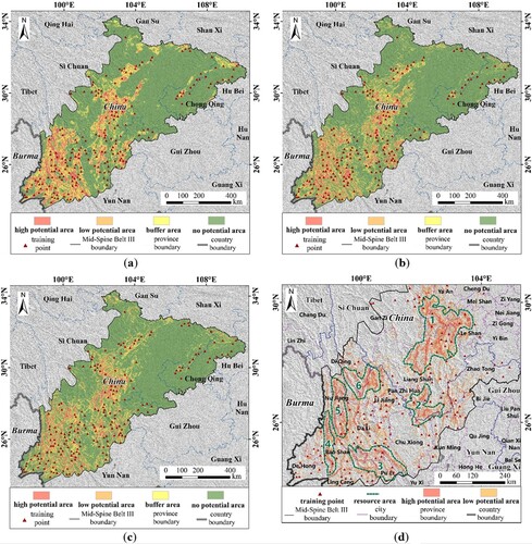
It can be seen from the prediction potential grading diagram and statistical results that the overall prediction results of the three models are relatively close, but there are local differences. On the whole, the geothermal high potential areas are concentrated in the southwest and central regions of the southwest section of the middle ridge belt, with a north–south trend, and these areas are mostly located in China's terrestrial seismic belt. Combined with various factors, the high potential area is characterized by high LST, a dense water system, developed plate tectonics, complex stratigraphic lithology and frequent earthquakes. In terms of details, the prediction results of the ECF are more precise, and the spatial correlation between low potential area and high potential area is stronger.

According to the predicted results of the ECF, six geothermal resource areas can be identified (Figure 8(d)): (1) Ganzi–Yaan–Liangshan geothermal resource areas: located in Ganzi Tibetan autonomous prefecture in the east and extends to the south of the Yaan and Jintang fault zone in the west of the Leshan and Mount Emei–Yibin Anling River fault zone in northwest and Liangshan Yi autonomous prefecture, the fresh water river fault zone and the Hanyuan–Ganluo fault zone. The north and south direction on the whole covers an area of 6791.63 km², making it the largest of the geothermal resource areas. Among them, Emeishan–Yibin fault zone and Anning River fault are lithosphere and superlithosphere faults. Xianshuihe fault is in the active period after the strong active period of the fault. The Yangtze, Xianshuihe, Anning and Polong Rivers flow through the area. (2) Panzhihua–Liangshan geothermal resource area: The Panzhihua fault in the east of Panzhihua city runs in a north–south direction, covering an area of about 1640.39 km². Yalong River and its tributary Anning River flow through the area. (3) Dali–Chuxiong geothermal resource area:The southwestern border southeast of Dali Bai minority autonomous prefecture and Chuxiong Yi nationality autonomous prefecture of Honghe fault and fracture, Ailaoshan assumes the northwest–southeast direction and covers an area of 2450.92 km². The ritual club river basin is in the Simao area of South China plate and Yangtze platform, introducing a Caledonian fold belt of docking. (4) Nujiang–Baoshan geothermal resource area: The Nujiang Lisu Autonomous Prefecture in the west extends to the Nujiang Fault in the middle of Baoshan City, with a north–south trend and an area of about 1142.3 km², which is the smallest geothermal resource area. The Nujiang river basin in the area is located in the subduction zone of Baoshan Block and Tengchong Block of Gondwana Plate. (5) the Diqing–Dali geothermal resource area: the Diqing Tibetan autonomous prefecture to the Nujiang Lisu autonomous prefecture in southwest and central Dali Bai minority autonomous prefecture in the west of the lancang river fault, the north–south, covers an area of 2303.91 km², and the area of Lancang river basin is in the midst of the Gondwana plate of Baoshan Block and South China plate of Simao Massif plate butt. (6) Lijiang–Diqing geothermal resource area is located in the northwest of Lijiang and Diqing Tibetan autonomous prefecture in the southeast border Jinsha river faults and small river fracture in the northwest–southeast and northeast to southwest, respectively, covers an area of 1923.09 km². The Jinsha river basin is in the South China plate of Simao Massif, Zhongdian Indosinian fold belt, Yangtze platform of docking.

4.2. Model assessment

4.2.1. Kappa consistency

Kappa coefficient analysis is a method to express the relationship between models and is mostly used to test the consistency between prediction results and experimental results. The method is based on a confusion matrix and adopts multivariate discrete theory to measure accuracy and test consistency (Cohen 1960; Li et al. 2009). The calculation formula of the Kappa coefficient is as follows: (19) $K={\displaystyle \frac{P_0-P_e}{1-P_e}}$(19) where P₀ is the observed consistency rate; P_e is the coincidence rate of opportunity.

Kappa consistency analysis was performed on the three models, and the results were as follows (Table 4):

Table 4. Predicted results kappa coefficient.

	CF						kappa
ICF	Class	1	2	3	4	Total	0.624
	1	44911320	2276856	101914	0	47290090
	2	2173165	3207022	1725845	18040	7124072
	3	273809	1202086	2771222	921472	5168589
	4	0	31150	436405	1819831	2287386
	Total	47358294	6717114	5035386	2759343	61870137
ECF	Class	1	2	3	4	Total	0.619
	1	45016433	3133049	1225399	85734	49460615
	2	1757168	3214461	468285	330527	5770441
	3	506989	274844	3119681	562848	4464362
	4	77704	94760	222021	1780234	2174719
	Total	47358294	6717114	5035386	2759343	61870137
	ICF
ECF	Class	1	2	3	4	Total	0.643
	1	44984820	3096922	1289969	88904	49460615
	2	1788695	3486882	470826	24038	5770441
	3	498917	480944	3253834	230667	4464362
	4	77704	94760	222021	1780234	2174719
	Total	47290090	7124072	5168589	2287386	61870137

As can be seen from Table 4, the predicted results of the ICF and the ECF are highly consistent, with the Kappa coefficient reaching 0.643. In summary, the kappa coefficients of the three models are substantially consistent, and the prediction results are close.

4.2.2. Analysis of success index

The success index method involves dividing the geothermal points in each grade of the predicted results by the total number of grids in that grade and comparing the success index with the prior probability (0.00034%) to analyze the accuracy of the predicted results. From the calculation results (table 5), it can be seen that with the increase in potential, the value of the success index gradually increases, and the incidence of geothermal spots continues to increase. The success index value of the high potential area and medium potential area is much higher than the a priori probability, and the success index value of the no-potential area is lower than the a priori probability, indicating that the prediction results of the three models are reliable. Among them, the success index value of the ECF is larger in the high potential area and medium potential area, indicating that its prediction results are more accurate.

Table 5. Success indices from the classification maps of prediction.

Class	CF			ICF			ECF
	Grids	Points	Index	Grids	Points	Index	Grids	Points	Index
4	2759343	91	0.00330%	2287386	82	0.00358%	2174719	88	0.00405%
3	5035386	51	0.00101%	5168589	57	0.00110%	4464362	49	0.00110%
2	6717114	31	0.00046%	7124072	38	0.00053%	5770441	33	0.00057%
1	47358294	38	0.00008%	47290090	34	0.00007%	49460615	41	0.00008%

4.2.3. Analysis of area ratio

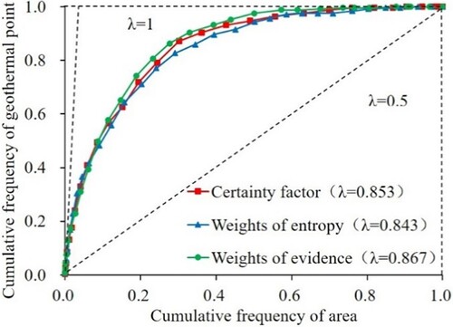
Area ratio analysis evaluates the effectiveness of the model by calculating the area under the curve of the predicted probability function (Lee and Talib 2005). In this method, the values of model prediction results are divided into 30 grades from large to small, the number of hotspots and layer area in each grade are counted, the cumulative frequency of grid and cumulative frequency of hotspots are calculated, and the prediction probability function and area ratio are obtained.

The calculation formula of area ratio is: (20) $\lambda =(2A-P)/(2-2P)$(20) where λ is the area ratio of the model; P is prior probability and A is the area bounded by the predicted probability function and the X-axis. The calculation results of area ratio are shown in Figure 9. The closer the area ratio to 1, the higher the accuracy of model prediction results. The area ratios of the three models are 0.853, 0.843 and 0.865, and the overall accuracy is similar. The accuracy of the ECF is slightly higher than the other two models.

Figure 9. Curves of prediction ratio function and its area ratio.

5. Discussion

The overall prediction results of the three models are relatively close, although local differences exist, and the ECF is the best. Its high potential area is 21747.19 km², including 88 geothermal hotspots, and 64.93% of geothermal training points are distributed in high potential areas and medium potential areas; that is, most geothermal hotspots are distributed in areas with high prediction potential. According to the results of the model, the southwest section of the MSBBC is indeed rich in geothermal resources, which is in line with the distribution of geothermal resources in Southwest China. The geothermal high potential areas are concentrated in the southwest and central regions of the southwest section of the middle ridge belt, and most of them have a north–south trend. These areas are also located in China's terrestrial seismic belt. The geothermal resource areas are Ganzi–Yaan–Liangshan geothermal resource area, Panzhihua–Lian–shan geothermal resource area, Dali–Chuxiong geothermal resource area, Nujiang–Baoshan geothermal resource area, Diqing–Dali geothermal resource area and Lijiang–Diqing geothermal resource area. In these areas, fault structures and river systems are highly developed, LST is high, plate tectonics are developed, stratigraphic lithology is complex, and earthquakes occur frequently.

The influencing factors are closely related to the spatial distribution of the observed hotspots: the hotspots are distributed more in the areas with high LST, high fault density, proximity to water systems and faults, high combined entropy, frequent earthquakes, low aeromagnetic anomaly and high Bouguer gravity anomaly. The input layer of the model fully considers all kinds of natural and geological factors that affect the occurrence of geothermal high-temperature anomalies and avoids the one-sidedness of the single factor.

By using the information entropy theory and the evidence weight theory, the deterministic coefficient method is improved, which can more accurately and objectively characterize the difference of geothermal influence factors. The CF could not reflect the different effects of various factors on the occurrence of geothermal high temperature anomalies. In the ICF and ECF, each impact factor has an objective weight value to characterize its geothermal impact. In the calculation results of entropy weight, the weight of LST, fault density and distance from water system is larger. The weight of LST and fault density is high in the calculation results of evidence weight. Combined with the two models, LST and faults are the key factors for judging geothermal high temperature anomaly areas, which represent terrestrial heat flow and geological structure. Kappa coefficient analysis showed that the CF, ICF and ECF had high consistency in prediction results. The results show that the weighted certainty coefficient model can effectively predict the geothermal potential area and can also provide ideas for groundwater resource evaluation and prediction, collapse, landslide, fire risk evaluation, pollution risk evaluation and other fields.

6. Conclusions

In this study, the method of deterministic coefficient was optimized, the geothermal resource potential area of the southwest section of the MSBBC was quantitatively predicted and a good result was obtained, which provides a basis for the effective development and utilization of geothermal resources in southwest China and a new idea for the sustainable development mode and method of the MSBBC. This approach will help to improve the energy structure in western China, boost the local economy and achieve the dual carbon target. However, there are still some shortcomings in this study, especially that the geothermal resource areas are only classified at a larger scale. The Sustainable Development Goals Science Satellite 1 (SDGSAT-1) successfully launched by China in 2021 has a thermal infrared payload of 30 m resolution, which is the highest spatial resolution in China at present, and has a width of 300 km. It can provide high-precision long-wave infrared data of the global surface. Future research will use the data to invert the LST of geothermal resource areas and achieve their fine characterization.

Acknowledgments

We would like to offer special thanks to NASA and USGS for providing us with the Landsat8 images. We also thank the China Geological Survey and the Digital Hu Line Research Institute of Chengdu University of Technology for the support of research area and various data they provided. A special acknowledgement should be expressed to International Research Centre of Big Data for Sustainable Development Goals (CBAS) that supported the implementation of this study.

Disclosure statement

No potential conflict of interest was reported by the author(s).

Data availability statement

The data that support the findings of this study are openly available in Dryad Digital Repository at https://doi.org/10.5061/dryad.6t1g1jx0z.

Additional information

Funding

This research was funded by National Key Research and Development Program of China (2017YFC0601500, 2017YFC0601502), Strategic Priority Research Program of the Chinese Academy of Sciences (grant number XDA19090121), National Natural Science Foundation of China (42002298) and Key Research and Development Program of Sichuan Provincial Science and Technology Department (2022YFS0486).

References

- Abdel-Fattah, M. I., E.-A. H. Shendi, and M. F. Kaiser. 2020. “Unveiling Geothermal Potential Sites Along Gulf of Suez (Egypt) Using an Integrated Geoscience Approach.” Terra Nova 33: 306–319. doi:10.1111/ter.12516.
- Abuzied, S. M., M. F. Kaiser, and E. Shendi. 2020. “Multi-criteria Decision Support for Geothermal Resources Exploration Based on Remote Sensing, GIS and Geophysical Techniques Along the Gulf of Suez Coastal Area, Egypt.” Geothermics 88: Article 101893. doi:10.1016/j.geothermics.2020.101893.
- Aydogan, D. 2011. “Extraction of Lineaments from Gravity Anomaly Maps Using the Gradient Calculation: Application to Central Anatolia.” Earth, Planets and Space 63: 903–913. doi:10.5047/eps.2011.04.003.
- Becker, F., and Z. L. Li. 1990. “Temperature-independent Spectral Indices in Thermal Infrared Bands.” Remote Sensing of Environment 32: 17–33. doi:10.1016/0034-4257(90)90095-4.
- Cao, W. C., H. P. Tao, B. Kong, B. T. Liu, and Y. L. Sun. 2011. “Automatic Identification of Geomorphology Partition of Southwest China Based on DEM Data.” Soil and Water Conservation in China 348: 38–41. doi:10.14123/j.cnki.swcc.2011.03.001.
- Chen, Z., Q. Dong, J. P. Chen, W. B. Zhao, L. W. Jiang, and G. Z. Zhang. 2021. “Research on Quantitative Prediction and Evaluation of Geothermal Anomaly Area in Qamdo-Nyingchi Section of Sichuan–Tibet Railway.” Remote Sensing Technolgy and Application 36: 1–11. doi:10.11873/j.issn.1004-0323.2021.3.0001.
- Chen, J. P., P. Lu, W. Wu, and H. Q. Zhao. 2017. “A 3D Method for Predicting Blind Orebodies, Based on a 3D Visualization Model and its Application.” Frontiers in Earth Science 47: 1819–1828. doi:10.3321/j.issn:1005-2321.2007.05.006.
- Chi, S. D., and P. D. Zhao. 2000. “Application of Combined-Entropy Anomany of Geological Formations to Delineation of Preferable Ore-Finding Area.” Geoscience, 423–428. doi:10.3969/j.issn.1000-8527.2000.04.006.
- Cohen, J. 1960. “A Coefficient of Agreement for Nominal Scales.” Educational and Psychological Measurement 37–46. doi:10.1177/001316446002000104.
- Crespo, E., J. Lillo, R. Oyarzun, P. Cubas, and M. Leal. 2013. “The Mazarron Basin, SE Spain: A Study of Mineralization Processes, Evolving Magmatic Series, and Geothermal Activity.” International Geology Review 55: 1978–1990. doi:10.1080/00206814.2013.810379.
- Cristóbal, J., J. C. Jiménez-Muñoz, A. Prakash, C. Mattar, D. Skoković, and J. A. Sobrino. 2018. “An Improved Single-Channel Method to Retrieve Land Surface Temperature from the Landsat-8 Thermal Band.” Remote Sensing 10 (3): 431. doi:10.3390/rs10030431.
- El Bouazouli, A., L. Baidder, P. Pasquier, and S. Rhouzlane. 2019. “Remote Sensing Contribution to the Identification of Potential Geothermal Deposits: A Case Study of the Moroccan Sahara.” Materials Today: Proceedings 13: 784–794. doi:10.1016/j.matpr.2019.04.041.
- Fan, L. F., R. L. Hu, F. C. Zeng, S. S. Wang, and X. Y. Zhang. 2012. “Application of Weighted Information Value Model to Landslide Susceptibility Assessment-A Case Study of Enshi City, Hubei Province.” Journal of Engineering Geology 20: 508–513. doi:10.3969/j.issn.1004-9665.2012.04.005.
- Hedlund, B. P., J. K. Cole, and A. J. Williams. 2012. “A Review of the Microbiology of the Rehai Geothermal Field in Tengchong,Yunnan Province, China.” Geoscience Frontiers 3: 273–288. doi:10.1016/j.gsf.2011.12.006.
- Hou, J. 2013. “Spatial Assessment for Groundwater Quality Based on GIS and Improved Fuzzy Comprehensive Assessment with Entropy Weights.” Chinese Journal of Population, Resources Environment 11: 135–141. doi:10.1080/10042857.2013.800384.
- Ian, M. 1992. “Earthquake Hazard Analysis: Issues and Insights.” Surveys in Geophysics 8: 635–636. doi:10.1193/1.1585699.
- Institute of Geography, CAS. 2015. Atlas of Qinghai–Tibet Plateau. Beijing: Science Press.
- Jiang, M., H. D. Tan, and Y. W. Zhang. 2012. “Geophysical Mode of Mazhan – Gudong Magma Chamber in Tengchong Volcano- Tectonic Area.” Acta Geoscientica Sinica 33 (5): 731–739. doi:10.3975/cagsb.2012.05.03.
- Jiménez-Muñoz, J. C., and J. A. Sobrino. 2003. “A Generalized Single-Channel Method for Retrieving Land Surface Temperature from Remote Sensing Data.” Journal of Geophysical Research Atmospheres 108), doi:10.1029/2003JD003480.
- Jin, D. D., and Z. N. Gong. 2018. “Algorithms Comparison of Land Surface Temperature Retrieval from Landsat Series Data: A Case Study in Qiqihar, China.” Remote Sensing Technology and Applications 33: 830–841. doi:10.11873/j.issn.1004-0323.2018.5.0830.
- Johnson, L. R. 2014. “Source Mechanisms of Induced Earthquakes at the Geysers Geothermal Reservoir.” Pure and Applied Geophysics 171: 1641–1668. doi:10.1007/s00024-014-0795-x.
- Lee, S., and J. A. Talib. 2005. “Probabilistic Landslide Susceptibility and Factor Effect Analysis.” Environmental Geology 47: 982–990. doi:10.3724/SP.J.1047.2017.01593.
- Li, G. L., P. J. Du, X. M. Wang, and L. S. Yuan. 2009. “Consistency Evaluation and Integration Application of Land Cover Classification Results from Multi-Source Remotely Sensed Images.” Geography and Geo-Information Science 25: 68–71. doi:JournalArticle/5af3a4c5c095d718d80f0698.
- Li, J. M., and Y. J. Zhang. 2018. “GIS Based Information Model for Assessment of Geothermal Potential: Case Study of Tengchong County, Southwest China.” Journal of Engineering Geology 26: 540–550. doi:10.13544/j.cnki.jeg.2017-010.
- Liu, Y. 2003. “Risk Analysis and Zoning of Geological Hazards (Chiefly Landslide, Rock Fall and Debris Flow) in China.” The Chinese Journal of Geological Hazard and Control 1: 98–102. doi:10.3969/j.issn.1003-8035.2003.01.020.
- Liu, Z. T., J. Ding, J. H. Qin, and W. Y. Fan. 2010. “Status of Copper Resources in Southwestern China and Suggestion on Prospecting.” Geological Bulletin of China 184: 1371–1382. doi:10.3969/j.issn.1671-2552.2010.09.014.
- Mcguire, J. J., R. B. Lohman, R. D. Catchings, M. J. Rymer, and M. R. Goldman. 2015. “Relationships among Seismic Velocity, Metamorphism, and Seismic and Aseismic Fault Slip in the Salton Sea Geothermal Field Region.” Geophysical Research Solid Earth 120: 2600–2615. doi:10.1002/2014JB011579.
- Qin, Z. H., M. H. Zhang, and K. Arnon. 2001. “Mono-window Algorithm for Retrieving Land Surface Temperature from Landsat TM6 Data.” Acta Geographica Sinica 456–466. doi:10.1142/S0252959901000401.
- Ren, X. M. 2012. “Study on the Estimation of b Value on Seismic Zontion.” Recent Developments in World Seismology 397: 32–330. doi: CNKI:SUN:GJZT.0.2012-01-012.
- Revil, A., and P. A. Pezard. 1998. “Streaming Electrical Potential Anomaly Along Faults in Geothermal Areas.” Geophysical Research Letters 25: 3197–3200. doi:10.1029/98GL02384.
- Shannon, C. E., and W. Weaver. 1947. The Mathematical Theory of Communication. Urbana: The University of Illinois Press. doi:10.1002/j.1538-7305.1948.tb00917.x.
- Shortliffe, E. H. 1975. “A Model of Inexact Reasoning in Medicine.” Mathematical Biosciences 23: 351–379. doi:10.1016/0025-5564(75)90047-4.
- Sobrino, J., J. C. Jiménez-Muñoz, and L. Paolini. 2004. “Land Surface Temperature Retrieval from LANDSAT TM 5.” Remote Sensing Environment 90: 434–440. doi:10.1016/j.rse.2004.02.003.
- Tang, G. A., and X. Yang. 2004. Experimental Course of Spatial Analysis of ArcGIS. Beijing: Science Press.
- Tangestani, M. H., and F. Moore. 2002. “Porphyry Copper Potential Mapping Using the Weights-of- Evidence Model in a GIS, Northern Shahr-e-Babak, Iran.” Australian Journal of Earth Sciences 48: 695–701. doi:10.1046/j.1440-0952.2001.485889.x.
- Vlassova, L., F. Perezcabello, M. Mimbrero, R. M. Llovería, and A. García-Martín. 2014. “Analysis of the Relationship Between Land Surface Temperature and Wildfire Severity in a Series of Landsat Images.” Remote Sensing 6: 6136–6162. doi:10.3390/rs6076136.
- Wan, Z. M., and Z. L. Li. 1997. “A Physics-Based Algorithm for Retrieving Land-Surface Emissivity and Temperature from EOS/MODIS Data.” IEEE Transactions on Geoscience and Remote Sensing 35: 980–996. doi:10.1109/36.602541.
- Wang, D. F. 2013. Aeromagnetic Series Maps and Specifications of Qinghai–Tibet Plateau and Adjacent Areas. Beijing: Geological Publishing House.
- Wang, X. Y., H. D. Guo, L. Luo, and R. C. Cang. 2021. “From Hu Huanyong Line to Mid-Spine Belt of Beautiful China:Breakthrough in Scientific Cognition and Change in Development Mode.” Proceedings of the Chinese Academy of Sciences 36: 1058–1065. doi:10.16418/j.issn.1000-3045.20210729002.
- Wang, J. Y., Z. H. Pang, Y. L. Kong, Y. Z. Cheng, and J. Luo. 2020. “Status and Prospects of Geothermal Clean Heating Industry in China.” Science & Technology for Development 16: 294–298. doi:10.11842/chips.20200516002.
- Wang, N., H. Wu, F. Nerry, C. R. Li, and Z. L. Li. 2001. “Temperature and Emissivity Retrievals from Hyperspectral Thermal Infrared Data Using Linear Spectral Emissivity Constraint.” IEEE Transactions on Geoscience and Remote Sensing 49: 1291–1303. doi:10.1109/TGRS.2010.2062527.
- Watson, T., F. A. Kruse, and M. S. Hummer. 1990. “Thermal Infrared Exploration in the Carlin Trend.” Geophysics 55: 70–79. doi:10.1190/1.1442773.
- Yan, J., C. He, B. Wang, W. Meng, and F. Y. Wu. 2019. “Inoculation and Characters of Rock Bursts in Extra-Long and Deep Tunnels Located on Yarlung Zangbo Suture.” Chinese Journal of Rock Mechanics and Engineering: 769–781. doi:10.13722/j.cnki.jrme.2018.1038.
- Yan, B. Z., S. W. Qiu, C. L. Xiao, and X. J. Liang. 2017. “Potential Geothermal Fields Remote Sensing Identification in Changbai Mountain Basalt Area.” Journal of Jilin University (Earth Science Edition) 47: 1819–1828. doi:10.13278/j.cnki.jjuese.201706205.
- Yang, Y. T., and Y. Y. Wang. 2014. “A Continuous Fuzzy Weight-of-Evidence Model for Mineral Potential Mapping.” Geography and Geo-Information Science 30: 41–45. doi:10.3969/j.issn.1672-0504.2014.06.009.
- Yuliang, Q., and Y. Yongming. 2008. “Method Studies in Exploring Underground Heat Water Using Infrared Remote Sensing.” Meteorological and Environmental Sciences 31 (4): 3. doi:10.3969/j.issn.1673-7148.2008.04.003.
- Zhang, X. M. 2019. “Hazard Assessment and Zoning Research of Landslide in Shanxi Province Based on GIS.” Chang’an University.
- Zhang, F. W., G. L. Wang, X. W. Hou, J. H. Li, and Y. J. Li. 2000. “An Analysis of the Formation of Geothermal Resources and the Effects of Groundwater Circulation on the Wall Rock Temperature Field-Taking the Pingdingshan Mining Field as an Example.” Acta Geoscientia Sinica21: 142–146.
- Zhang, P. M., and J. L. Zhang. 2006. “Identification of Remote Sensing Information in Geothermal Abnormal Area.” Remote Sensing Information 2: 42–45. doi:10.3969/j.issn.1000-3177.2006.02.013.
- Zhao, P. D., and S. D. Chi. 1991. “Preliminary View on Geological Anomaly.” Earth Science – Journal of China University of Geosciences16: 241–248.
- Zhao, W. B., Q. Dong, Z. Chen, T. Feng, D. Wang, L. Jiang, S. Du, X. Zhang, M. Bian, and D. Meng. 2021. “Weighted Information Models for the Quantitative Prediction and Evaluation of the Geothermal Anomaly Area in the Plateau: A Case Study of the Sichuan–Tibet Railway.” Remote Sensing 13: 1606. doi:10.3390/rs13091606.
- Zhao, H., and E. X. Song. 2011. “Improved Information Value Model and Its Application in the Spatial Prediction of Landslides.” Journal Architecture Civil Engineering Environment33: 38–44. doi:10.3969/j.issn.1674-4764.2011.03.007.
- Zhou, Z. Y., S. L. Liu, and J. X. Liu. 2015. “Study on the Characteristics and Development Strategies of Geothermal Resources in China.” Journal of Natural Resources 30: 1210–1221. doi:10.12849/zrzyxb.2015.07.013.
- Zhou, Z. H., C. Y. Xiang, and W. M. Deng. 1997. “Lithospheric Geothermal Structure in Yunnan, China.” Earthquake Research in China 13 (3): 213–223. doi:CNKI: SUN: ZGZD.0.1997-03-002.