A topological framework for real-time 3D weather radar data processing

ABSTRACT

Real-time 3D weather radar data processing makes it possible to efficiently simulate meteorological processes in digital Earth and support the assessment of meteorological disasters. The current real-time meteorological operation system can only deal with radar data within 2D space as a flat map and lacks supporting 3D characteristics. Thus, valuable 3D information imbedded in radar data cannot be completely presented to meteorological experts. Due to the large amount of data and high complexity of radar data 3D operation, regular methods are not competent for supporting real-time 3D radar data processing and representation. This study aims to perform radar data 3D operations with high efficiency and instant speed to provide real-time 3D support for the meteorological field. In this paper, a topological framework composed of basic inner topological objects is proposed along with the quadtree structure and LOD architecture, based on which 3D operations on radar data can be conducted in a split second and 3D information can be presented in real time. As the applications of the proposed topological framework, two widely used 3D algorithms in the meteorological field are also implemented in this paper. Finally, a case study verifies the applicability and validity of the proposed topological framework.

KEYWORDS:

• Weather radar data
• 3D operations
• real-time
• topological framework

1. Introduction

Strong convective weather can cause much loss of life and property (Xue 2016; Meng et al. 2019; Shi, Cui, and Shen 2020). With the development of the digital Earth, virtual geographic environment (VGE) and 3D geographic information science (GIS), it has been possible to simulate real-time convective weather processes in 3D environments and provide great support for decision-making in meteorological fields. However, limited by the computing power of hardware, real-time processing and visualization of 3D meteorological data are still a challenge for related fields.

Currently, people can observe convective clouds and watch their development over time by Doppler radar systems (Zheng et al. 2017; Sun et al. 2019; Zheng et al. 2019; Vogl et al. 2021). The current presentation of radar data in regard to convective clouds is limited within 2D space as a flat map (Roberts and Rutledge 2003; Chen et al. 2012; Cică, Burcea, and Bojariu 2015; Lee, Kummerow, and Zupanski 2021), which omits much three-dimensional (3D) information about convective clouds, such as the 3D shape characteristics imbedded in radar data, and causes barriers for the identification and judgment of severe convective weather. Radar data contain 4D spatiotemporal characteristics (Choi, Cha, and Kim 2017; Sindhu and Bhat 2018; Oue et al. 2019; Gao et al. 2021), and with the development of 3D GIS and spatiotemporal GIS (Petrov et al. 2015; Kim and Chung 2020; Van Pham 2020; RRC and DHM 2021), they can be visualized and analyzed in 3D or 4D geoenvironments to explore much more valuable information about convective clouds (Mbogo, Rakitin, and Visheratin 2017; Rautenhaus et al. 2018; Kim and Hong 2019; Pálenik, Spengler, and Hauser 2021; Mahavik, Tantanee, and Masthawee 2021). However, 3D operations are resource consuming, and regular methods are not competent to support real-time 3D radar data processing and representation in meteorological fields. Therefore, 3D presentation and analysis have not been provided in radar data real-time observation systems thus far (Lu et al. 2018). How to rapidly conduct 3D operations on radar data has become a key issue in the meteorological field.

In recent years, studies on 3D data indices and visualization operations of weather radar data have been carried out (Ernvik 2002; d'Agostino, Clematis, and Gianuzzi 2011; Yang et al. 2011; Lu, Jin, and Han 2013; Guan et al. 2015; Han et al. 2016; Liu et al. 2017; Lu et al. 2017). Lu, Jin, and Han (2013) reconstructed and visualized a 3D convective cell based on radar data. Lu et al. (2018) proposed a 3D modeling strategy to represent and analyze weather radar data. Guan et al. (2015) conducted 3D visualization of radar data based on the MATLAB platform. Liu et al. (2017) implemented 3D image reconstruction and visualization for weather radar data.

Meanwhile, some software products (such as Unidata’s integrated data viewer (IDV 2021) and the autonomous visualization system (AVS)) also provide excellent tools to display and analyze 3D radar data. All these studies have achieved great progress in the 3D processing of radar data. In these studies, regular 3D grids have often been used to analyze 3D radar data; that is, the radar data are interpolated into regular 3D grids first, and then the related algorithms are carried out on regular 3D grids to obtain 3D results. Due to the large number of 3D grids and the operational complexity, most studies have focused more on the methods to obtain 3D products and have given little attention to the operational efficiency, especially for real-time applications. Thus, these achievements can hardly be applied in real-time meteorological operation systems.

To solve this problem, a topological framework along with the quadtree structure, which is a spatial data structure built by a recursive decomposition of space into quadrants, and the layer of detail (LOD, which can be considered the scale to display the representation or the scale at which the phenomena can be meaningfully analyzed) architecture for real-time radar data processing are proposed in this paper, based on which 3D radar data operations and algorithms can be conducted in real time.

The rest of this paper is organized as follows. In Section 2, we provide the details of constructing the topological framework and its spatial organization strategies. Section 3 is dedicated to the implementation of the real-time processing algorithms based on the topological framework. In Section 4, we present the experimental setup and results. Finally, we conclude and discuss future research directions in Section 5.

2. The topological framework and its construction

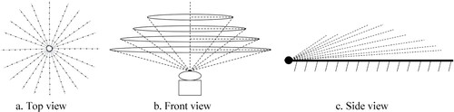
Doppler radar scans the 3D space around it repeatedly to obtain a series of data. Therefore, the 3D space the Doppler radar scans can be rebuilt by the spatial points, which are structured consistently with the volume-scan mode of Doppler radar (by sweeps and lines, as shown in Figure 1). To support 3D data analysis, other geometric objects, such as irregular quads and hexahedrons, together with their topological relationships, are also built based on these points. Thus, a topological framework composed of these various types of geometric objects with topological relationships is proposed to meet diverse 3D operation requirements, in which the points are regarded as the basic carriers to load the radar data. At the same time, spatial Octree and LOD organization strategies are also set up in the framework to improve the situation. With the aid of the topological framework and organization strategies, the 3D operations of radar data can be conducted with high efficiency and can provide significant support for meteorological real-time systems.

Figure 1. The radar space of the weather radar volume-scan (Lu et al. 2017).

2.1 The basic topological objects and their construction in the framework

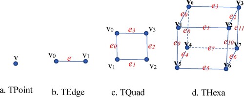
In the proposed framework, there are four basic topological geometry objects: topological point (namely, TPoint), topological edge (namely, TEdge), topological quadrangle (namely, TQuad) and topological hexahedron (namely, THexa). The TPoint is the primary object that truly carries the radar data in the framework. TEdge is actually the intermediate object that is used to assist operations in processing. TQuad is one final topological object in the framework and is used to construct continuous quadrangle grids to carry out some surface operations. THexa is another final topological object in the framework and is used to construct continuous hexahedron grids to carry out some volumetric operations.

In construction, they have their own intrinsic rules and data structures to support topological relationships and operations (as shown in Figure 2). The TPoint is the basic object used to construct other topological objects. In addition to the position and attribute value, a TPoint also contains topological relationships with its associated TEdges, TQuads and THexas. TEdge is constructed by two TPoints (as shown in Figure 2b) and contains topological relationships with its associated TQuads and THexas. As a final object, TQuad is constructed by four TPoints (as shown in Figure 2c), but it also contains the information of its associated four TEdges. In constructing a TQuad, four TPoints should be stored in a certain order and anticlockwise order is adopted in this paper, and the TEdges in a TQuad should also be in the same order; that is, the TEdge between v₀ and v₁ should be the first TEdge(e₀), the TEdge between v₁ and v₂ should be the second TEdge(e₁), and the TEdge between v₃ and v₀ should be the last TEdge(e₃). THexa is another final object in the topological framework; it is constructed by eight TPoints and contains the information of 12 TEdges. In construction, eight TPoints should be connected in a certain order to generate a THexa (as shown in Figure 2d). On the upper side, four TPoints (v₀, v₁, v₂, and v₃) are connected in anticlockwise order, and the TEdges (e₀, e₁, e₂, and e₃) are also in the same order. On the lower side, four TPoints (v₄, v₅, v₆, and v₇) are connected in the same order, and the TEdges (e₄, e₅, e₆, and e₇) are also in the same order. Meanwhile, v0 and v4 are connected as e₈, v₁ and v₅ are connected as e₉, v₂ and v₆ are connected as e₁₀, and v₃ and v₇ are connected as e₁₁. In the construction of the final objects (TQuad and THexa), the connection order is critical for subsequent operations. There are two other variables contained in the final topological objects: one is the bounding box for quick spatial collision detection, and the other is the max–min-value (MMV), which is the maximum value and minimum value of all TPoints in the final objects for fast value detection. The full definitions of topological objects in the framework are shown as follows:

TPoint = { P, Es, Qs, Hs, Value}

Where

Figure 2. The basic geometric objects with their construction in the topological framework.

P: The position of this TPoint

Es: The topological edges associated with this TPoint

Qs: The TQuads associated with this TPoint

Hs: The THexas associated with this TPoint

Value: The attribute value (radar reflectivity value in this research) attached to this TPoint

TEdge = {Ps, Qs, Hs}

Where

Ps: The TPoints associated with this edge

Qs: The TQuads associated with this edge

Hs: The THexas associated with this edge

TQuad =  {Ps, Es, AABB, MMV}

Where

Ps: The TPoints associated with this TQuad

Es: The topological edges associated with this TQuad

Aabb: The bounding box of this TQuad

Mmv: The maximum value and minimum value of all TPoints in this TQuad

THexa =  {Ps, Es, AABB, MMV}

Where

Ps: The TPoints associated with this THexa

Es: Topological edges associated with this THexa

Aabb: The bounding box of this THexa

Mmv: The maximum value and minimum value of all TPoints in this THexa

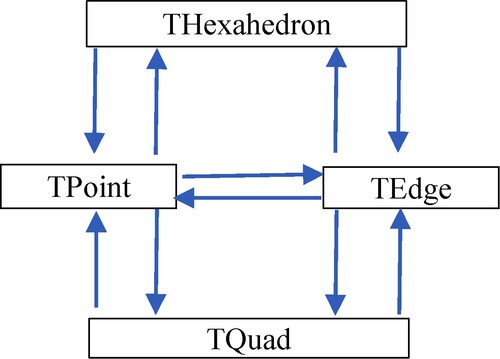
As mentioned above, the topological relationships among the four basic objects are very flexible (as shown in Figure 3). The final topological objects can also be considered constructed by both TPoints and TEdges, which make it very convenient to find the associated objects from each other and make the operations very efficient; however, at the cost of redundancy. This is also the compromising strategy in this paper.

Figure 3. The topological relationships among the four basic objects.

2.2 Construction of the topological framework

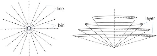
In the framework, the four basic topological objects are well constructed with specific topological structures. Every topological object must be unique in the framework to maintain the validity of the topological relationships. Therefore, some rules and tricks should be used in their constructions. Spatially, all Tpoints are arranged according to the volume-scan mode of Doppler radar (by sweeps and lines), as shown in Figure 4. That is, all Tpoints are arranged in several layers (sweeps) with different elevations; in each layer, the Tpoints are arranged in 360 lines, and each line contains approximately 460 bins (here, the bin can be regarded as the location of Tpoint). Therefore, TPoints are constructed based on their spatial locations and stored by the structure of a 3D array in which the first dimension refers to the layer index, the second dimension refers to the line index, and the third dimension refers to the bin index. Therefore, each TPoint can be indicated by the array index. For example, TPoints[i][j][k] can be located at the No. i layer, No. j line, and No. k bin. All TPoints constructed are unique in the topological framework and used to construct other objects.

Figure 4. The Tpoint arrangement in the framework.

TEdges in the framework are divided into 3 types: Row_TEdge, Col_TEdge and Wall_TEdge. Row_TEdge is the TEdge constructed by two TPoints from the same radar line. Col_TEdge is the TEdge constructed by two TPoints from two adjacent radar lines in the same layer. Wall_TEdge is constructed by two corresponding TPoints from two adjacent layers. The three types of TEdges are built separately and stored in 3D array structures. Thus, according to the TPoint arrangement rules, the three types of TEdges can be constructed as follows:

Row_TEdge[i][j][k]  = {TPoint[i][j][k], TPoint[i][j] [K+1] }

Where

0 <= K < binSize-1

Binsize: The amount of data on the radar line in layer i.

Col_TEdge[i][j][k]  = {TPoint[i][j][k], TPoint[i][j+1] [K]}

Where

If (j+1 = radar lines amount), then j+1 = 0.

Wall_TEdge[i][j][k] = {TPoint[i][j][k], TPoint[i+1] [j][k]}

Where

0 <= i < layerSize -1

Layersize: The radar layer amount.

In the construction of TEdges, the topological relationships between TPoints and TEdges are also completed.

As final objects, TQuads and THexa are constructed by both TPoint and TEdge. Meanwhile, they are also stored in a 3D array structure separately. Therefore, after constructing TPoints and TEdges in the topological framework, TQuads[i][j][k] and THexas[i][j][k] can be built as follows:

TQuad[i][j][k] = {v₀, v₁, v₂, v₃, e_0, e_1, e_2, e_3, e_4, }

Where

v₀ = TPoint[i][j+1] [k] v₁ = TPoint[i][j+1] [k+1]

v₂ = TPoint[i][j] [k+1] v₃ = TPoint[i][j][k]

e₀= Row_Edges[i][j+1] [k] e₁= Col_Edges[i][j] [k+1]

e₂ = Row_Edges[i][j][k] e₃= Col_Edges[i][j][k]

THexa[i][j][k] = {v₀, v₁, v₂, v₃, v₄, v₅, v₆, v_7, e_0, e_1, e_2, e_3, e_4, e_5, e_6, e_7, e_8, e_9, e_10, e₁₁}

Where

v₀ = TPoint [i+1] [j+1] [k]    v₁= TPoint[i+1] [j+1] [k+1]

v₂ = TPoint[i+1] [j][k+1]     v₃ = TPoint[i+1] [j][k]

v₄ = TPoint[i][j+1] [k]      v₅ = TPoint[i][j+1] [k+1]

v₆ = TPoint[i][j] [k+1]      v₇ = TPoint[i][j][k]

e₀ = Row_Edges[i+1] [j+1] [k]  e₁ = Col_Edges[i+1] [j][k+1]

e₂ = Row_Edges[i+1] [j][k]     e₃ = Col_Edges[i+1] [j][k]

e₄= Row_Edges[i][j+1] [k]     e₅= Col_Edges[i][j] [k+1]

e₆ = Row_Edges[i][j][k]      e₇= Col_Edges[i][j][k]

e₈ = Wall_Edges[i][j+1] [k]     e₉ = Wall_Edges[i] [ j+1] [k+1]

e₁₀ = Wall_Edges[i][j] [k+1]     e₁₁= Wall_Edges[i][j][k]

In the above formulas, the parameters i, j and k should meet the following limitation conditions:

if (j+1 = lineSize), then j+1 = 0

0 <= i < layerSize -1

0 <= K < binSize-1

After construction, the relationships among TPoints, TEdges and THexas are complemented, and all topological objects are stored separately in their 3D array structures. Therefore, the primary topological framework with basic connected objects is also built successfully.

The topological framework is composed of TPoints, TEdges and THexas together with their mutual connections. However, extra organization strategies are also required to enhance the capabilities of dealing with 3D operations. Thus, quadtree structures and layer of detail (LOD) strategies are also designed to meet the requirements.

2.3 The quadtree structure in the topological framework

In most operations, qualified objects should be located quickly. However, it would consume much time due to the number of objects in the framework. Thus, the quadtree structure is adopted in this paper to speed up this process.

In the framework, TPoints are the actual objects carrying the radar data; therefore, TPoints are taken as the objects organized in the quadtree structure. The qualified TEdges, TQuads and THexas can be located quickly through topological connections with the qualified TPoints. The layer (sweep) amount is much less than the bin amount; that is, the height in the Z-axis is much less than the length and width in the XY-axis in 3D space. Therefore, this paper adopts the quadtree, not octree, as the organization strategy.

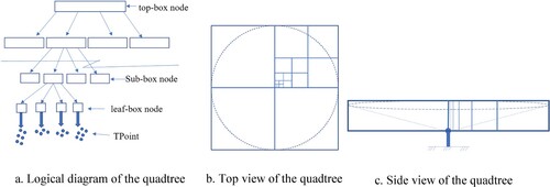
Actually, the radar volumetric-scan space is similar to a cone and a circle from the top view. Thus, the quadtree can be designed as shown in Figure 5. The top-box node covers all 3D space; then, it is separated into four subbox nodes, and each subbox node is separated into another four subbox nodes. The subbox nodes in the bottom level can be called leaf-box nodes (as shown in Figure 5a). All TPoints in the topological framework are allotted to the leaf-box nodes in the quadtree. In each quadtree box node, there are 2 types of parameters: spatial information and data value information.

Figure 5. The quadtree designed in the topological framework.

The data value information of each box node includes the maximum and minimum data values attached to the TPoints that belong to this box node.

The spatial information includes the spatial region of the box node: the maximum and minimum values of height, longitude and latitude. In this paper, all box nodes have the same height. The height range (MinHeight, MaxHeight) can be calculated by the following formulas:

MinHeight = radarH

MaxHeight = radarH + lineLen * sin(ele) + lineLen²/(1.21 * 2 * EarthRadius)

Where

Minheight: The bottom height of the box node, kilometer (km)

Maxheight: The top height of the box node, km

Radarh: The height of the radar antenna, km

Linelen: The length of the line on the top sweep, km

Ele: The elevation of the top sweep, radian

Earthradius: The radius of Earth, which is 6371 km

The spatial range of the top box can be calculated by the following formulas:

Dis = bottomLineLen * cos(bottomEle); (1)

MaxLon = radarLat + Dis/(π* EarthRadius)*180 (2)

MaxLat = radarLon + Dis/(π* EarthRadius*cos(MaxLon * π/180))*180 (3)

MinLon = radarLat - Dis/(π* EarthRadius) * 180 (4)

MinLat = radarLon - Dis/(π* EarthRadius * cos(MaxLon *π/180))*180 (5)

Where

Dis: The intermediate variable used to calculate the final result, km

Maxlon: The maximum longitude of the box node, degree

Maxlat: The maximum latitude of the box node, degree

Minlon: The minimum longitude of the box node, degree

Minlat: The maximum latitude of the box node, degree

Radarlat: The latitude of the radar antenna, degree

Radarlon: The longitude of the radar antenna, degree

Earthradius: The radius of Earth, which is 6371 km

Thus, the boundary of the subbox nodes under the top-box node can also be calculated according to the top-box node. If the parent box node boundary is [minLon_super, maxLon_super, minLat_super, maxLat_super], then its four subbox node boundaries of [minimum longitude, maximum longitude, minimum latitude, maximum latitude] can be calculated as follows:

Northeast subbox node:

[(minLon_super + maxLon_super)/2, maxLon_super, (minLat_super + maxLat_super)/2, maxLat_super]

Northwest subbox node:

[minLon_super, (minLon_super + maxLon_super)/2, (minLat_super + maxLat_super)/2, maxLat_super]

Southwest subbox node:

[minLon_super, (minLon_super + maxLon_super)/2, minLat_super, (minLat_super + maxLat_super)/2]

Southeast subbox node:

[(minLon_super + maxLon_super)/2, maxLon_super, minLat_super, (minLat_super + maxLat_super)/2]

After the above process, the quadtree can be constructed successfully. In addition, each TPoint can find its right node to stay.

2.4 Lod strategy in the topological framework

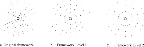
Products based on the current topological framework possess all the detailed information, but the amount of data is also enhanced, which places a great burden on data transportation and visualization, especially in real-time applications. In the meteorological field, detailed information is not always necessary, and sparse information can also meet the requirements well in most scenarios. Therefore, this article employs the LOD (layer of detail) strategy to represent data with different levels of detail. Based on the topological framework, the TPoints are chosen every two (three, four or more) bins in each line (as shown in Figure 6). Then, a new topological framework can be generated with these chosen TPoints, in which the TPoint amounts are much less than those in the original framework. Accordingly, other topological objects together with the connections among them can also be constructed in the same way, as well as the quadtree structure in the new topological framework. Thus, new topological frameworks with fewer data can be constructed for less detailed products. In this way, a hierarchy of various topological frameworks with different levels of data amounts are generated to meet different application scenarios: in subtle scenarios, operations can be conducted in the original topological framework to obtain detailed products, and in general scenarios, operations can be rapidly conducted in shrunken frameworks to obtain less detailed products with less data and better efficiency of data transmission and visualization. In applications, topological frameworks at different detailed levels can be prebuilt in advance to support 3D radar data operations.

Figure 6. Schematic diagram of LOD for the topological frameworks.

3. Real-time processing algorithms based on the topological framework

The constructed topological framework possesses great potential to support radar data 3D operations in real-time scenarios. For its applications, two widely used 3D algorithms in the meteorological field are chosen as examples to demonstrate how to implement the 3D operations efficiently based on the topological framework.

3.1 3d isosurface extraction algorithm

3D isosurface extraction is a fundamental operation for 3D data analysis and visualization (Newman and Yi 2006). In this paper, 3D isosurfaces can be extracted from THexas in the topological framework through the marching cubes (MC) algorithm (Cercos-Pita et al. 2018; Newman and Yi 2006), which is one of the most widely used algorithms for isosurface extraction (Lorensen and Cline 1987; Liu et al. 2017) and has been implemented in various open-source toolkits, such as the Visualization Toolkit (VTK 2021) and the Autonomous Visualization System (AVS 2021). The time consumption of the MC algorithm increases with the growth of the data size. Therefore, how to rapidly find the actual THexas that are exactly involved in generating 3D isosurfaces is the key issue for achieving real-time processing.

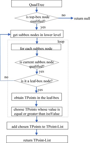
With the help of the quadtree structure and the topological relationships in the framework, qualified THexas can be located immediately. In this paper, the extraction of the 3D isosurface can be conducted through 3 main steps: 1. find possible TPoints that may be involved in the algorithm based on the quadtree structure; 2. find the qualified THexas based on the topological relationship with the possible TPoints found in Step 1; and 3. 3D isosurface extraction based on the MC algorithm. The detailed steps are as follows:

1. Find the possible TPoints (as shown in Figure 7):

   1. Define the value of the 3D isosurface as the isoValue.

   2. Define the criteria to indicate the qualified box node in the quadtree. If the isoValue is between the minimum value and maximum value reserved in the box node, then the box node is qualified.

   3. Check the top-box node in the quadtree. If the top box is not qualified, then there are no possible TPoints in the current framework; otherwise, check its four subbox nodes and find the qualified subbox nodes.

   4. Recursively traverse the qualified subbox nodes until all qualified box nodes are leaf-box nodes.

   5. Obtain the TPoints contained in the qualified leaf-box nodes and filter out those whose values are less than the isovalue.

   6. The remainder are the possible TPoints and are added to a list (namely, TPoints-List).

2. Identifying the qualified THexas

   1. Define the criteria to indicate the qualified THexa:

If the isoValue is between the minimum value and maximum value reserved in the THexa, then the THexa is qualified.

1. Traverse all possible TPoints in TPoints-List and perform the following steps:

   • i. According to the criteria defined in Step a, obtain the qualified THexas associated with the current TPoint;

   • ii. Uniquely store the qualified THexas in a list (namely, THexas-List).

2. All qualified THexas in THexas-List are exactly involved in the 3D isosurface algorithm.

Figure 7. Flow chart of finding the possible TPoints based on the quadtree.

• 3. Carry out the MC algorithm on the qualified THexas in THexas-List.

Taking advantage of the quadtree structure and the topological connection between the TPoints and THexas in the framework, the invalidated THexas that are not exactly involved in the MC algorithm can be filtered out quickly, and therefore, the operation is sped up to a great extent.

3.2 Vertical profile extraction algorithm

The vertical profile is an important pattern for exploring the inner structure of volumetric data. The vertical profile extraction algorithm, operated on volumetric cells such as tetrahedrons and hexahedrons, is relatively mature (Pietroni et al. 2009). In this paper, based on the THexas together with the topological connection in the topological framework, the qualified THexas and TEdges can be located quickly, and the cutting point on each TEdge can be calculated only once, avoiding multiple calculations when it is shared in different THexas. Therefore, the vertical profile extraction algorithm can be conducted much more efficiently. Taking advantage of the topological characteristics, the vertical profile can be achieved through two fundamental steps: 1) find the qualified THexas that are definitely cut by the cutting plane; and 2) obtain the cutting facets on the cutting plane. The detailed steps are described as follows:

1.

Find the qualified THexas cut by the cutting plane. Find the first THexa(H0) that is exactly cut by the cutting plan, add H0 to a list (namely, THexa-list), traverse all topological TEdges associated with H0 to find the qualified TEdges that are exactly cut by the cutting plane, and push the qualified TEdges into a queue (namely, TEdge-queue). At the same time, label all associated TEdges to indicate that they are settled. Pop a TEdge (E) from TEdge-queue, conduct a cutting operation between E and the cutting plane to obtain the coordinates and appropriate value of the cutting point, and then save them inside E. Traverse the topological THexas associated with E; if one (Hi) is not in the THexa-list but in the bounding box of the cutting plane, add it (Hi) to the THexa-list. Then, traverse the topological TEdges associated with Hi. If one is not labeled and it is the qualified TEdge that is exactly cut by the cutting plane, then push it into the TEdge-queue and label it to indicate that it is settled. Repeat Steps b and c until the TEdge-queue is empty; then, the THexas in the THexa-list are all qualified.

2. Obtain the cutting facets on the cutting plane

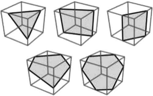
There are five basic types of intersections between the cutting plane and a THexa (Byeon and Lee 2021) (as shown in Figure 8). The cutting facets on each THexa can be obtained according to the specific intersection type. Therefore, we can traverse all THexas in the THexa-List and obtain the cutting facets on each THexa one by one according to the following:

1. For one THexa, find its qualified TEdges cut by the cutting plane according to the intersection point calculated in the previous steps, and record their index numbers in the THexa.

2. According to the index numbers of the qualified TEdges in the THexa, a specific type of intersection can be matched according to Figure 7.

3. With the specific intersection type, cutting facets on this THexa can be achieved.

Figure 8. The basic intersection types between a plane and hexahedron.

The previous steps on each THexa in THexa-list are repeated, and a vertical cutting profile with various facets can be achieved. With the values on the vertices of the facets, the profile can be drawn on the screen. This part is relatively mature in the GIS field and not the core of this paper; therefore, no detailed descriptions are presented here.

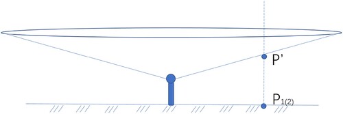
In the above steps, a key technical problem should be solved first; that is, how to obtain the first qualified THexa that is exactly cut by the cutting plane. To solve this problem, assuming a cutting plane of the vertical profile is defined by two points (P₁, P₂) on the ground (as shown in Figure 9), a virtual point (P’) with the same longitude and latitude as P₁ (or P₂) is set in the first radar data layer (as shown in Figure 10), and then the distance and azimuth between P’ (with coordination [lonP’, latP’]) and the position (with coordination [lonR, latR]) of the radar antenna can be calculated by the following formula:

arcdst = arccos(sin(latR) * sin(latP’) +cos(latR) *cos(latP’) * cos ((lonR – lonP’)));

Dis = EarthRadius * arcdst/cos(sweepAngle0);

Azi = arccos((sin(LatP)- sin(latR) * cos(arcdst))/(cos(latR) *sin(arcdst)));

Where

Figure 9. The cutting plane defined by P₁ and P₂.

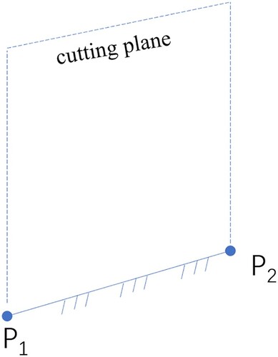
Figure 10. The relationship between P₁₍₂₎ and P’.

Arcdst: The intermediate data

Dis: The distance between P’ and the radar antenna

Sweepangle0: The sweep angle of the first layer (0.5 degrees in this paper)

Azi: The azimuth of point P according to the radar antenna

Then, according to the characteristics of the 3D array structure that stores the THexas in the topological framework, the index of the THexa that contains point P’, also the first qualified THexa cut by the cutting plane, should be [i, j, k], in which

I= 0

j =int((Dis-firstBinLen)/binLen)

K = int(Azi)

Where

I: The first dimension in the 3D array structure in which the THexas are stored.

J: The second dimension in the 3D array structure in which the THexas are stored.

K: The third dimension in the 3D array structure in which the THexas are stored

Firstbinlen: The first bin length in the first radar data layer

Binlen: The bin length in the first radar data layer

4. Experiment and results

An experiment is conducted to verify the viability and efficiency of the proposed topological framework in real-time radar data processing. In the experiment, the S band Doppler radar is utilized to realize the framework. For the radar reflectivity data, a volume scan of the Doppler radar can generate 9 sweeps with elevations of 0.5°, 1.45°, 2.4°, 3.35°, 4.30°, 6.0°, 9.9°, 14.6°, and 19.5°. Thus, according to the parameters of the Doppler radar, the topological framework can be constructed by the following steps: 1) determine the center of the framework according to the position of the Doppler radar; 2) determine the points organized in layers and lines around the center of the framework; 3) construct the basic topological objects (TPoints, TEdges, TQuads and THexas) with their topological relationships according to Section 2.1; 4) build the QuadTree structure to organize the Tpoints in the framework according to Section 2.3; and 5) construct another two less detailed topological frameworks (LOD framework Level 1 and LOD framework Level 2) according to Section 2.4. The construction of the total topological framework set consumes approximately 6 s, and it needs to be carried out only once at the beginning of the whole process. Afterward, the radar data are parsed from the radar archive files and attached to the constructed topological frameworks. Then, the 3D isosurfaces with 9 value layers (with radar reflectivity values of 20, 25, 30, 35, 40, 45, 50, 55 and 60 dbz) are extracted based on different detailed frameworks. Meanwhile, a conventional method based on regular 3D grids is also implemented to generate 3D isosurfaces with the same 9 value layers. All these results from different strategies are displayed on the virtual weather Earth system built based on the browser/server (B/S) architecture to represent and analyze meteorological data in a virtual 3D geoenvironment.

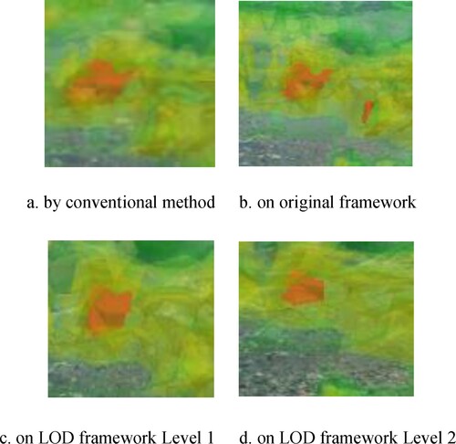
In this experiment, a laptop equipped with an Intel® Core™ i7-6820HQ CPU @ 2.7 GHz, 16 GB RAM and a 512 GB SSD is installed with Windows 10 professional 64 Bits, Java10, Intellij Idea 2018.3.2 and Visual Studio Code 1.63.0. The results generated in different strategies are very close, as shown in Figure 11. The slight differences in the results can be found in Figure 12.

Figure 11. The isosurfaces based on different strategies.

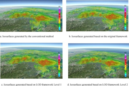
Figure 12. The details in isosurfaces based on different strategies.

The consumption time and the product data amount based on different strategies vary greatly, as listed in Table 1.

Table 1. Consumption time and isosurface data amount based on different strategies.

strategy	all triangles counted in product data	average consumption time (ms)
conventional method	675864	2537.6
the original topological framework	171443	230.1
LOD framework Level 1	91401	69.4
LOD framework Level 2	63005	42.7

The 3D isosurface extraction operations based on the original topological framework spend much less time than those based on the conventional method. Additionally, based on less detailed frameworks, the 3D isosurface operation consumes increasingly less time and generates much less triangle data, which can be transferred and rendered much faster in practical real-time applications. Thus, based on the proposed topological framework, the whole process of the isosurface extraction operation is sped up and suitable for real-time application.

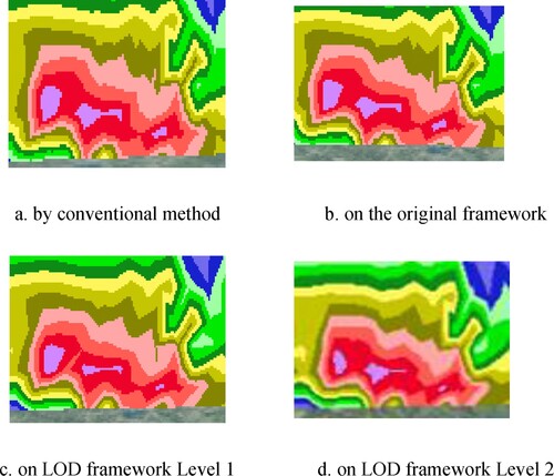
Meanwhile, vertical profiles are also achieved with high efficiency based on topological frameworks. The time consumed by the operation based on the different-level, detailed topological framework is much shorter than that based on the conventional method. The results are presented on the virtual weather Earth system (as shown in Figure 13). The results are also very close, and some slight differences in details are shown in Figure 14.

Figure 13. The vertical profiles based on different strategies.

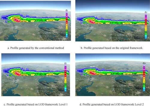
Figure 14. The details in vertical profiles based on different strategies.

A comparison of the consumption time and the facet amount in the profile product data based on different strategies is also provided in Table 2.

Table 2. The consumption time and facet amount in profiles based on different strategies.

strategy	all facets counted in profile data	average consumption time (ms)
conventional method	6237	836.4
the original topological framework	4687	58.5
LOD Framework Level 1	3445	36.5
LOD Framework Level 2	2976	30.1

The above two cases both achieve proper results with significant efficiency based on the proposed topological framework, which also proves the validity and adaptability of the proposed topological framework.

At the same time, five more cases are also adopted in this paper to verify the efficiency of the algorithms based on the proposed topological framework. The consumption times of 3D operations on the basis of both conventional methods and different levels of topological frameworks in different cases are shown in Tables 3 and 4. The operations based on conventional methods consume much more time than on the proposed topological frameworks, and the LOD strategy also has an important effect on these operations and can reduce much consumption time in these cases.

Table 3. The consumption time of 3D isosurface extraction based on different strategies in more cases.

consumption time in each case (ms) strategy	Case 1 (ms)	Case 2 (ms)	Case3 (ms)	Case 4 (ms)	Case 5 (ms)	Average (ms)
conventional method	2207	2147	2345	2271	2081	2210.2
original topological framework	122	118	125	115	111	118.4
LOD Framework Level 1	58	49	51	51	45	50.7
LOD Framework Level 2	48	39	40	35	40	40.5

Table 4. The consumption time of 3D vertical profile extraction based on different strategies in more cases.

consumption time in each cases(ms) strategy	Case 1 (ms)	Case 2 (ms)	Case3 (ms)	Case 4 (ms)	Case 5 (ms)	Average (ms)
conventional method	803.4	752.6	1005.5	702.9	822.3	817.3
original topological framework	53.6	60.8	52.8	44	53.8	53.0
LOD Framework Level 1	27.2	31	27.6	27.2	29	28.4
LOD Framework Level 2	17.2	20	15.6	12.4	15.2	16.1

According to the experiments conducted above, it is obvious that taking advantage of the topological characteristics and LOD architecture, the proposed topological framework can provide powerful and flexible support to 3D operations in real time for different application scenarios and possesses competitive potential for the spatiotemporal simulation and visualization of convective weather in the meteorological field.

5. Conclusions and discussion

This paper proposes a topological framework composed of some basic topological objects with complete connections to process 3D radar data with high efficiency. Meanwhile, the quadtree structure and LOD architecture are also achieved in the topological framework. With the support of the preconstructed framework, 3D operations on radar data can be conducted in real time. A case study in this paper also demonstrates the applicability of the proposed topological framework and its high efficiency in 3D operations. Therefore, real-time 3D products from radar data can become common materials for meteorologists in their decision-making process regarding severe weather, which would greatly compensate for the deficiency of current 2D products in the meteorological field. In this paper, the topological framework is stable, while the radar data are changeable and can be attached to the framework frequently. Thus, with the competence of real-time 3D weather radar data processing, this topological framework possesses great potential to represent and simulate spatiotemporal climate events and enables good exploration for geographic process simulation in the digital Earth or virtual geographic environment (VGE) fields. Based on the topological framework proposed in this paper, identifying storm cells and tracking them to simulate the process of thunderstorms and forecasting severe weather are our next research goals.

Acknowledgments

Many thanks to reviewers for their valuable comments. This paper was supported by the NSFC Project (41871285).

Data availability statement

The data that support the findings of this study are available from the first author Lu, upon reasonable request.

Disclosure statement

No potential conflict of interest was reported by the author(s).

Additional information

Funding

This work was supported by National Natural Science Foundation of China: [Grant Number 41871285].

References

- AVS (The autonomous visualization system). 2021. https://avs.auto/#/. (accessed on 29 October 2021).
- Byeon, S. P., and D. Y. Lee. 2021. “Adaptive Surface Representation Based on Homogeneous Hexahedrons for Interactive Simulation of Soft Tissue Cutting.” Computer Methods and Programs in Biomedicine 200: 105873.
- Cercos-Pita, J. L., I. R. Cal, D. Duque, and G. S. de Moreta. 2018. “NASAL-Geom, a Free Upper Respiratory Tract 3D Model Reconstruction Software.” Computer Physics Communications 223: 55–68.
- Chen, M., Y. Wang, F. Gao, and X. Xiao. 2012. “Diurnal Variations in Convective Storm Activity Over Contiguous North China During the Warm Season Based on Radar Mosaic Climatology.” Journal of Geophysical Research: Atmospheres 117 (D20): 20.
- Choi, Y., D. H. Cha, and J. Kim. 2017. “Tuning of Length-Scale and Observation-Error for Radar Data Assimilation Using Four Dimensional Variational (4D-Var) Method.” Atmospheric Science Letters 18 (11): 441–448.
- Cică, R., S. Burcea, and R. Bojariu. 2015. “Assessment of Severe Hailstorms and Hail Risk Using Weather Radar Data.” Meteorological Applications 22 (4): 746–753.
- d'Agostino, D., A. Clematis, and V. Gianuzzi. 2011. “Parallel Isosurface Extraction for 3D Data Analysis Workflows in Distributed Environments.” Concurrency and Computation: Practice and Experience 23 (11): 1284–1310.
- Ernvik, A. 2002. 3d visualization of weather radar data.
- Gao, S., N. Du, J. Min, and H. Yu. 2021. “Impact of Assimilating Radar Data Using a Hybrid 4DEnVar Approach on Prediction of Convective Events.” Tellus A: Dynamic Meteorology and Oceanography 73 (1): 1–19.
- Guan, L., M. Wei, K. Wei, and J. Wang. 2015. “3D Visualization of Doppler Radar Data Based on MATLAB Platform.” Journal of Henan Normal University 43: 43–48.
- Han, Y., X. Liu, X. Lu, H. Li, and R. Wu. 2016. “The 3D modeling and radar simulation of low-altitude wind shear via computational fluid dynamics method.” In 2016 Integrated Communications Navigation and Surveillance (ICNS) (pp. 4D3-1).
- IDV(Integrated Data Viewer). 2021. https://www.unidata.ucar.edu/software/idv/. (accessed on 29 October 2021).
- Kim, M., and C. K. Chung. 2020, August. Development of a GIS-Based System for Three-Dimensional Spatial Modeling of Offshore Site Investigation Information. In International Conference on Offshore Mechanics and Arctic Engineering (Vol. 84423, p. V010T10A017). American Society of Mechanical Engineers.
- Kim, Y., and S. Hong. 2019. “Convective Cloud RGB Product and Its Application to Tropical Cyclone Analysis Using Geostationary Satellite Observation.” Journal of the Korean Earth Science Society 40 (4): 406–413.
- Lee, Y., C. D. Kummerow, and M. Zupanski. 2021. “A Simplified Method for the Detection of Convection Using High-Resolution Imagery from GOES-16.” Atmospheric Measurement Techniques 14 (5): 3755–3771.
- Liu, Z., Z. Shi, M. Jiang, J. Zhang, L. Chen, T. Zhang, and G. Liu. 2017. “Using MC Algorithm to Implement 3d Image Reconstruction for Yunnan Weather Radar Data.” Journal of Computer and Communications 05 (5): 50–61.
- Lorensen, W. E., and H. E. Cline. 1987. “Marching Cubes: A High Resolution 3D Surface Construction Algorithm.” ACM Siggraph Computer Graphics 21 (4): 163–169.
- Lu, M., M. Chen, X. Wang, J. Min, and A. Liu. 2017. “A Spatial Lattice Model Applied for Meteorological Visualization and Analysis.” ISPRS International Journal of Geo-Information 6 (3): 77.
- Lu, M., M. Chen, X. Wang, M. Yu, Y. Jiang, and C. Yang. 2018. “3D Modelling Strategy for Weather Radar Data Analysis.” Environmental Earth Sciences 77 (24): 1–10.
- Lu, Z. Y., X. Jin, and C. Y. Han. 2013. 3D reconstruction of Strong Convective Cell Based on Doppler Radar Base Data. In 2013 International Conference on Machine Learning and Cybernetics (Vol. 2, pp. 845-849). IEEE.
- Mahavik, N., S. Tantanee, and F. Masthawee. 2021. Investigation of ZR Relationships During Tropical Storm in GIS Using Implemented Mosaicking Algorithms of Radar Rainfall Estimates from Ground-Based Weather Radar in the Yom River Basin. Thailand: Applied Geomatics. 1–13.
- Mbogo, G. K., S. V. Rakitin, and A. Visheratin. 2017. “High-performance Meteorological Data Processing Framework for Real-Time Analysis and Visualization.” Procedia Computer Science 119: 334–340.
- Meng, Z., F. Zhang, D. Luo, Z. Tan, J. Fang, J. Sun, … Y. Zhu. 2019. “Review of Chinese Atmospheric Science Research Over the Past 70 Years: Synoptic Meteorology.” Science China Earth Sciences 62 (12): 1946–1991.
- Newman, T. S., and H. Yi. 2006. “A Survey of the Marching Cubes Algorithm.” Computers & Graphics 30 (5): 854–879.
- Oue, M., P. Kollias, A. Shapiro, A. Tatarevic, and T. Matsui. 2019. “Investigation of Observational Error Sources in Multi-Doppler-Radar Three-Dimensional Variational Vertical air Motion Retrievals.” Atmospheric Measurement Techniques 12 (3): 1999–2018.
- Pálenik, J., T. Spengler, and H. Hauser. 2021. “IsoTrotter: Visually Guided Empirical Modelling of Atmospheric Convection.” IEEE Transactions on Visualization and Computer Graphics 27 (2): 775–784.
- Petrov, V. A., A. V. Veselovskii, D. A. Kuz’mina, A. N. Plate, and T. V. Gal’berg. 2015. “Spatial-temporal Three-Dimensional GIS Modeling.” Automatic Documentation and Mathematical Linguistics 49 (1): 21–26.
- Pietroni, N., F. Ganovelli, P. Cignoni, and R. Scopigno. 2009. “Splitting Cubes: A Fast and Robust Technique for Virtual Cutting.” The Visual Computer 25 (3): 227–239.
- Rautenhaus, M., M. Böttinger, S. Siemen, R. Hoffman, R. M. Kirby, M. Mirzargar, … R. Westermann. 2018. “Visualization in Meteorology—a Survey of Techniques and Tools for Data Analysis Tasks.” IEEE Transactions on Visualization and Computer Graphics 24 (12): 3268–3296.
- Roberts, R. D., and S. Rutledge. 2003. “Nowcasting Storm Initiation and Growth UsingGOES-8and WSR-88D Data.” Weather and Forecasting 18 (4): 562–584.
- RRC, R., and D. DHM. 2021. A Spatial Temporal Classification Analysis and Visualization of Tropical Cyclone Tracks in Bay of Bengal using GIS.
- Shi, J., L. Cui, and Z. Shen. 2020. “Interannual Variation and Hazard Analysis of Meteorological Disasters in East China.” Journal of Risk Analysis and Crisis Response 9 (4): 168–176.
- Sindhu, K. D., and G. S. Bhat. 2018. “Characteristics of Monsoonal Precipitating Cloud Systems Over the Indian Subcontinent Derived from Weather Radar Data.” Quarterly Journal of the Royal Meteorological Society 144 (715): 1742–1760.
- Sun, J., J. Chai, L. Leng, and G. Xu. 2019. “Analysis of Lightning and Precipitation Activities in Three Severe Convective Events Based on Doppler Radar and Microwave Radiometer Over the Central China Region.” Atmosphere 10 (6): 298.
- Van Pham, D.. 2020. “Proposing Spatial - Temporal - Semantic Data Model Managing Genealogy and Space Evolution History of Objects in 3D Geographical Space". In Context-Aware Systems and Applications, and Nature of Computation and Communication (pp. 148-168). Springer, Cham
- Vogl, T., M. Maahn, S. Kneifel, W. Schimmel, D. Moisseev, and H. Kalesse-Los. 2021. “Using Artificial Neural Networks to Predict Riming from Doppler Cloud Radar Observations.” Atmospheric Measurement Techniques Discussions 15(2): 1–26.
- VTK (The Visualization Toolkit). 2021. http://public.kitware.com/VTK/ (accessed on 29 October 2021).
- Xue, M. 2016. “Preface to the Special Issue on the “Observation, Prediction and Analysis of Severe Convection of China” (OPACC) National “973” Projec.” Advances in Atmospheric Sciences 33 (10): 1099.
- Yang, C., H. Wu, Q. Huang, Z. Li, and J. Li. 2011. “Using Spatial Principles to Optimize Distributed Computing for Enabling the Physical Science Discoveries.” Proceedings of the National Academy of Sciences 108 (14): 5498–5503.
- Zheng, J., L. Liu, K. Zhu, J. Wu, and B. Wang. 2017. “A Method for Retrieving Vertical air Velocities in Convective Clouds Over the Tibetan Plateau from TIPEX-III Cloud Radar Doppler Spectra.” Remote Sensing 9 (9): 964.
- Zheng, J., P. Zhang, L. Liu, Y. Liu, and Y. Che. 2019. “A Study of Vertical Structures and Microphysical Characteristics of Different Convective Cloud–Precipitation Types Using Ka-Band Millimeter Wave Radar Measurements.” Remote Sensing 11 (15): 1810.