Combining post-disturbance land cover and tree canopy cover from Landsat time series data for mapping deforestation, forest degradation, and recovery across Cambodia

ABSTRACT

Mapping of deforestation, forest degradation, and recovery is essential to characterize country-level forest change and formulate mitigation actions. Previous studies have mainly used a simple forest/non-forest classification after forest disturbance to identify deforestation and forest degradation. However, a more flexible approach that is applicable to different forest conditions is desirable. In this study, we examined an approach for mapping deforestation, forest degradation, and recovery using disturbance types and tree canopy cover estimates from annual Landsat time-series data from 1988 to 2020 across Cambodia. We developed models to estimate both disturbance types and tree canopy cover based on a random forest algorithm using predictor variables derived from a trajectory-based temporal segmentation approach. The estimated disturbance types and canopy cover in each year were then used in a rule-based classification of deforestation, forest degradation, and recovery. The producer’s and user’s accuracies ranged from 59.1% to 72.9% and 60.8% to 91.6%, respectively, for the forest change classes of mapping deforestation, forest degradation, and recovery. The approach developed here can be adjusted for different definitions of deforestation, forest degradation, and recovery according to research objectives and thus has the potential to be applied to other study areas.

KEYWORDS:

• Deforestation
• degradation
• time series
• Google Earth Engine
• tropical forest

1. Introduction

Human-induced deforestation, forest degradation, and recovery in tropical forests critically affect local ecosystem services and benefits (Schaafsma et al. 2014), the global carbon cycle, and biodiversity (Mitchard 2018; Pan et al. 2011; Xu et al. 2021). In the past decades, increasing pressure from timber extraction, agricultural expansion, and other human activities have led to broad-scale deforestation and forest degradation (Lewis, Edwards, and Galbraith 2015). The spatial and temporal patterns of these forest changes differ considerably depending on the region and period (Baccini et al. 2017; Hansen et al. 2013). Therefore, the spatial and temporal monitoring of tropical forests is a vital step in quantifying these changes. Forest monitoring also has an important role in formulating mitigation actions within international frameworks such as Reducing Emissions from Deforestation and Forest Degradation and the role of conservation, sustainable management of forests and enhancement of forest carbon stocks in developing countries (REDD+) (Global Forest Observations Initiative 2020).

Medium-spatial-resolution optical satellite data have been widely used for regional and countrywide mapping of deforestation, forest degradation, and recovery because of their cost-effectiveness and wide area coverage (Finer et al. 2018; Mitchell, Rosenqvist, and Mora 2017; Miettinen, Stibig, and Achard 2014). Freely available satellite data, such as Landsat data, have enabled the development of long-term and large-scale spatial mapping in the last decade (Dupuis et al. 2020; Phiri et al. 2020; Wulder et al. 2015). One such example is the Global Forest Change (GFC) dataset generated by Hansen et al. (2013), which provides the annual global forest loss and recovery at 30 m spatial resolution. Although this dataset provides valuable information on forest change, forest loss in the dataset represents mostly deforestation, and thus further processing is required to separately map both deforestation and forest degradation. In addition, although a rigorous validation was implemented on the original dataset, as forest loss detection in the GFC data has been gradually improved, time series trend analysis might be problematic without rigorous validation for forest loss in the updated version of the dataset (Grassi, Cescatti, and Ceccherini 2021; Palahí et al. 2021; Shimizu, Ota, and Mizoue 2020). In terms of the global availability, the land cover map at 10 m resolution by the ESA WorldCover (Zanaga et al. 2021) using Sentinel-1 and Sentinel-2 data is promising; however, this map currently does not provide temporal change information. Therefore, accurate estimation of forest change requires the development of locally adjusted maps. Although many studies have developed methods for mapping deforestation, forest degradation, and recovery, the long-term trend in spatial and temporal patterns in the tropics has still not been investigated sufficiently; thus, suitable methods remain to be discovered especially at the country scale.

Many approaches using Landsat data have been proposed to detect deforestation and forest degradation in the tropics (e.g. Asner et al. 2005; Raši et al. 2011; Sannier, Fichet, and Makaga 2014; de Bem et al. 2020; Matricardi et al. 2010) caused by various drivers, such as agricultural development, logging, and fires (Geist and Lambin 2002; Hosonuma et al. 2012). However, the estimates of change areas still contain large uncertainty (Gao et al. 2020). This uncertainty mainly arises because it is difficult to monitor forest degradation despite its prevalence in tropical forests (Dupuis et al. 2020). Forest degradation is generally a process of gradual or subtle abrupt changes. Therefore, monitoring is more challenging than for deforestation (Gao et al. 2020). Furthermore, there are more than 50 definitions of forest degradation in the literature (e.g. "the reduction of the capacity of a forest to produce goods and services", FAO 2001) and the use of the term depends on the interests and goals of different projects (Morales-Barquero et al. 2014; Vásquez-Grandón et al. 2018). Although the indicators for assessing the degree of forest degradation, such as a forest degradation index (Modica et al. 2015; Wu et al. 2020), have been proposed in the literature, the optimal approaches also vary depending on the forest types, drivers, and data sources (Miettinen, Stibig, and Achard 2014). These situations have led to different approaches using Landsat data in previous studies, such as spectral mixture analysis (SMA, (Souza et al. 2013; Asner et al. 2005)), fragmentation of primary forests (Zhuravleva et al. 2013), and temporal changes of related indicators (Mon et al. 2012; Duarte et al. 2020). Time series analysis of Landsat data can provide important temporal information on forest conditions. This characteristic is suitable for detecting gradual and subtle changes from deforestation and forest degradation (Global Forest Observations Initiative 2020). Recent studies have successfully detected changes caused by selective logging, fire, and shifting cultivation using Landsat time series data (e.g. Shimizu et al. 2017; De Marzo et al. 2021; Vancutsem et al. 2021; Hethcoat et al. 2020).

Landsat time series analysis assesses the temporal change of indices, and it can be used in various ways for mapping deforestation and degradation. For example, Bullock, Woodcock, and Holden (2020b) used time series of spectral endmembers from SMA for detecting forest disturbance and estimating forest/non-forest land cover after disturbance to monitor deforestation and forest degradation. Other studies used the temporal changes of indices from Landsat time series for monitoring land cover change (Tang et al. 2020; Arévalo, Olofsson, and Woodcock 2020; Murillo-Sandoval et al. 2018), tree canopy cover (Potapov et al. 2019), and forest disturbances (Reygadas et al. 2021; Hamunyela et al. 2016; Aryal et al. 2021) and then related them to deforestation and forest degradation in the tropics. Previous studies have mainly used a simple forest/non-forest classification to identify deforestation and forest degradation; however, a more flexible approach is required because the definition and evaluation of both deforestation and forest degradation are complex. One possible approach is to use post-disturbance land cover classification. This approach allows us to investigate the drivers of deforestation (e.g. conversion to agriculture) and forest degradation (e.g. changes from natural forest to plantation). Additionally, the estimation of forest condition, such as tree canopy cover, after disturbance provides important implications for forest recovery (Hamunyela et al. 2020). Tree canopy cover estimation has proved to be successful in monitoring applications in previous studies because of its capacity to evaluate forest status (Potapov et al. 2019; Estoque et al. 2021). The continuous data provided by tree canopy cover can complement disturbance type classification, enabling the estimation of pre- and post-disturbance status. Such flexible characterization can provide useful information for both deforestation/degradation and vegetation recovery; however, few studies have mapped both types of change for entire countries to the best of our knowledge.

The main objective of this study was to develop an approach for mapping deforestation, forest degradation, and recovery using both post-disturbance land cover and tree canopy cover (TCC) estimated from Landsat time-series data in 1988–2020 for the whole of Cambodia. Our specific objectives were to (1) examine the accuracy of both post-disturbance land cover and TCC estimation using Landsat time-series data; (2) demonstrate the utility of an approach for mapping deforestation, forest degradation, and recovery using post-disturbance land cover and TCC; and (3) map countrywide spatial and temporal patterns of deforestation, forest degradation, and recovery.

2. Study area

The study area was the entire country of Cambodia, which has a total land area of 18.1 million ha between 10–15°N and 102–108°E. There is an annual dry season (November to April) and a rainy season (May to October) with a mean precipitation of 1780 mm and a mean temperature of 27°C. The forest in Cambodia consists mainly of evergreen, semi-evergreen (i.e. mixed evergreen/deciduous), deciduous, and flooded forests (Ministry of Environment Cambodia 2020).

Forest cover in Cambodia has declined over the past few decades (FAO 2020) from nearly 70% in the 1970s to 46.86% in 2018 (Ministry of Environment Cambodia 2020). The main causes of deforestation are agricultural land expansion and plantation development, whereas the causes of forest degradation include logging in forest concessions (Tsujino, Kajisa, and Yumoto 2019). Recent studies show that large-scale land acquisitions for agro-industrial use have contributed substantially to forest loss in Cambodia (Magliocca et al. 2020; Davis et al. 2015). To increase forest cover, several actions have been planned by the Cambodian government, including establishing Community Forestry and Protected areas, which are demonstrated to partially compensate forest loss (Ota, Lonn, and Mizoue 2020).

3. Methods

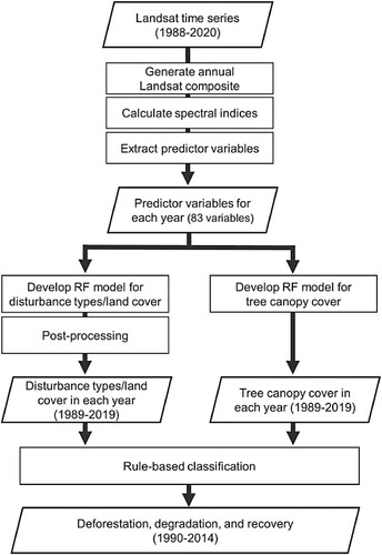
Annual estimates of forest disturbance types and TCC at a resolution of 30 m pixel were essential components for mapping deforestation, forest degradation, and recovery in this study (Figure 1). The main processing steps were to (1) preprocess Landsat time series to generate annual image composites; (2) extract predictor variables using the LandTrendr temporal segmentation algorithm (Kennedy, Yang, and Cohen 2010) and auxiliary data; (3) develop a random forest (RF) model to identify disturbance types and land cover classes in each year; (4) develop an RF model to estimate TCC in each year; and (5) identify deforestation, forest degradation, and recovery using a rule-based classification of disturbance type and TCC following disturbance. Finally, we assessed the accuracy of the two RF models and rule-based classification of deforestation, forest degradation, and recovery. In our approach, the results of temporal segmentation from the LandTrendr were used to derive the predictor variables of two RF models and then mapped disturbance types/land covers from RF models were subsequently used to predict deforestation, forest degradation, and recovery. Although our approach is different from the original algorithm, it can provide a locally adjustable way of mapping for the desired criterion.

Figure 1. Processing steps for mapping deforestation, forest degradation, and recovery.

3.1 Preprocessing of Landsat and topographic data

We used Landsat TM, ETM+, and OLI surface reflectance (SR) data (Masek et al. 2006; Vermote et al. 2016) acquired from October 1 to January 31 in 1988–2020 to minimize variations in vegetation phenology. We only selected SR data with a cloud cover of less than 70%. A quality assessment band generated by the CFmask algorithm (Zhu and Woodcock 2012; Zhu, Wang, and Woodcock 2015) was used to remove cloudy pixels. We transformed the spectral bands of Landsat OLI SR data to those of TM/ETM+ SR data using the coefficients of Roy et al. (2016) to compensate the spectral differences. We generated annual SR composites by calculating the median values in each year. Any gaps were filled with the mean SR values from the preceding and subsequent years at the same pixel locations. After preprocessing, we calculated the time series of the normalized burn ratio (NBR) (Key and Benson 2006) and the tasseled cap brightness (TCB), greenness (TCG), wetness (TCW), and angle (TCA) (Crist 1985) spectral indices using annual SR median composites. We used the digital elevation model from the Shuttle Radar Topography Mission (Farr et a. 2007) 1 arc-second (approximately 30 m) product to calculate topographic slope and elevation. We implemented all processing in Google Earth Engine (GEE) (Gorelick et al. 2017).

3.2. RF models of disturbance type/land cover classification and TCC

We used the same predictor variables for both RF models: one for identifying disturbance type and land cover classes and the other for estimating TCC. To derive predictor variables for each year, we followed the approach shown in (Shimizu et al. 2019; Shimizu and Saito 2021). This approach used LandTrendr temporal segmentation (Kennedy, Yang, and Cohen 2010), which fits several straight line segments for the time series of a spectral index, to extract variables representing spatial and temporal changes in each year. We used these extracted variables to model annual disturbance type/land cover and TCC estimation, unlike the original LandTrendr algorithm. As demonstrated in previous studies (e.g. Franklin et al. 2015), predictor variables from disturbance detection algorithms are useful to improve land cover classification. Based on the annual land cover classification, forest disturbances only occurred in forest areas, as described in the post-processing steps below. In this study, we used the five spectral indices for LandTrendr and derived a total of 83 variables related to vertex, magnitude, fitted, and original values for each spectral index (see Table S1 in Supplementary Materials).

We collected training data for the RF model that identified five disturbance types and five land cover classes (Table 1) using a combination of stratified random sampling and purposive procedures. For stratified random samples, we randomly selected pixel locations for stable forest (tree cover ≥ 10% in 2000), stable non-forest (tree cover < 10%), and forest loss (2001–2019) using the GFC data (Hansen et al. 2013). For purposive samples, we manually selected forest disturbances that occurred before 2000 and other disturbances/land cover classes that occupied small areas. To label the disturbance type/land cover class for each year, we used Landsat time-series data and high-spatial-resolution data from Google Earth Pro for visual interpretation (Figure 2). In a pixel time series, we randomly selected three sample years as training samples if there were no disturbances at the pixel locations. If a disturbance occurred in the time series, we selected three sample years (pre-disturbance, post-disturbance, and disturbance years) and two random years. This procedure was followed so we could balance the training samples across the study period.

Figure 2. Example of visual interpretation for disturbance type/land cover classification using (A) spectral indices derived from Landsat time series data, (B) RGB image chips of Landsat time series data, and (C) high-spatial-resolution data from Google Earth Pro (14.295°N, 104.369°E). Example of visual interpretation for tree canopy cover using (D) 3 × 3 regular spaced grid points in 30 m pixels on high-spatial-resolution data from Google Earth Pro (14.406°N, 106.611°E).

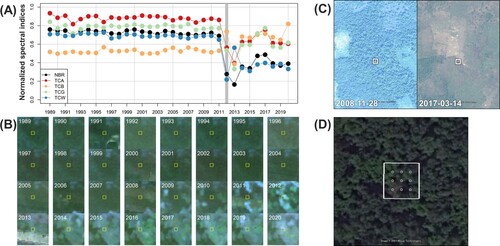
Table 1. Accuracy assessment for disturbance types/land cover classification based on 10 classes and 3 aggregated classes.

10 classes					3 classes
Class	Area (ha)	PA (%)	UA (%)	OA (%)	Class	Area (ha)	PA (%)	UA (%)	OA (%)
Natural forest	6,935,809	97.4 (±1.1)	77.1 (±3.1)	78.1 (±2.1)	Stable forest	7,150,761	96.4 (±1.3)	78.6 (±3.0)	87.2 (±1.6)
	(±281,050)					(±280,895)
Plantation	214,952	0.2 (±0.1)	28.0 (±10.2)
	(±99,169)
Agriculture	4,473,037	91.3 (±2.7)	78.9 (±3.9)		Other land cover	7,530,833	83.0 (±2.5)	94.6 (±1.8)
	(±240,740)					(±256,669)
Grass/Shrub	1,434,360	5.1 (±1.2)	61.3 (±11.1)
	(±241,231)
Urban/Water	1,623,436	70.6 (±6.6)	86.9 (±6.4)
	(±169,237)
Disturbance	1,516,987	63.9 (±6.5)	79.8 (±7.9)		Disturbance	3,449,222	77.2 (±4.2)	96.8 (±1.8)
(toAgriculture)	(±173,922)					(±192,918)
Disturbance	486,558	83.6 (±10.5)	68.0 (±10.6)
(toForest)	(±87,406)
Disturbance	780,292	46.1 (±8.1)	78.7 (±9.3)
(toGrass/Shrub)	(±134,533)
Disturbance	601,098	58.5 (±10.7)	76.0 (±9.7)
(toPlantation)	(±114,134)
Disturbance	64,287	23.7 (±17.8)	84.0 (±8.4)
(toUrban/Water)	(±48,051)

Note: Error-adjusted area, producer’s accuracy (PA) and user’s accuracy (UA) for each class, and overall accuracy (OA) are shown with 95% confidence intervals.

We selected a total of 1000 simple random pixel locations to train the RF model for estimating TCC. For each location, we manually labeled TCC in the years when high-spatial resolution satellite data were available in Google Earth Pro (Figure 2). We used 3×3 regular spaced grid points within 30 m pixels to label TCC, following the method in (Potapov et al. 2019). We calculated the proportion of nine sample grid points that intersected the tree canopy. If high-spatial-resolution data were not available, we removed such locations from training samples.

We fine-tuned the two RF models and applied them to all years over the entire study area using GEE. Because it is difficult to tune RF parameters in GEE in this analysis, we tuned the mtry parameter with 10-fold cross-validation using the package 'randomForest' (Liaw and Wiener 2002) and 'caret' (Kuhn 2008) in R statistical software (R Core Team 2021) and then used the obtained parameter in GEE with a number of trees of 500. The outputs of the RF models for disturbance types/land cover classes and TCC were a 10-class classification (Table 1 and Table S2 for detailed definitions) and tree cover (0–100%), respectively, for each year. For the results of disturbance types/land cover classes only, we applied post-processing steps to eliminate irrelevant land cover transitions. We removed disturbances that occurred in 2 consecutive years in the same pixel locations since two consecutive disturbances were unlikely. Then, we removed forest disturbances that had fewer than four spatially contiguous pixels in each year to reduce false disturbance detection. If the adjacent disturbances in spatially contiguous pixels had more than two disturbance types, we reclassified them to the majority disturbance types. If the land cover class changed without disturbances in a pixel time series, we allocated the majority of land cover classes to all years of the time series. If land cover classes before and after disturbance did not match the disturbance type, we reclassified such land cover classes to improve temporal consistency.

3.3 Mapping deforestation, forest degradation, and recovery

After mapping forest disturbance types/land cover and TCC annually from 1989 to 2019, we implemented a rule-based classification of deforestation, forest degradation, and recovery. In this study, we defined ‘deforestation’ as forest disturbances that resulted in conversion to non-forest, ‘forest degradation’ as a reduction in forest canopy cover compared with the original state, although the area remained forest, and ‘recovery’ as a state where forests reached the original canopy cover after forest disturbances. Forest disturbances were allocated to these three classes (i.e. deforestation, forest degradation, or recovery). To identify deforestation, we used forest disturbance types, which represented land covers following forest disturbances. Among the disturbance types, three (i.e. toAgriculture, toGrass/Shrub, and toWater/Urban) resulted in land cover conversion and thus were classified as deforestation. For other disturbances (i.e. toForest and toPlantation), we labeled these as either forest degradation or recovery based on the TCC after these disturbances. Since toPlantation in this study indicated the conversion of natural forests to rubber plantations (Table S2), we included this class as potentially recovered to forests, following the definition of forest by the FAO (2020). Forest recovery in this study required almost the same level of TCC before disturbance; thus, we defined a threshold value of 70% of original TCC as the forest recovery. When TCC reached 70% of the average values of the two years prior to disturbance (if two years were not available, TCC prior to disturbance) within 5 years after disturbance, we classified these as forest recovery. If TCC after disturbance did not reach this threshold, we regarded such cases as forest degradation. Since it required 5 years to identify forest degradation/recovery, we mapped deforestation, forest degradation, and recovery only from 1990 to 2014.

3.4. Spatial and temporal pattern of deforestation and forest degradation

We analyzed the spatial and temporal patterns of mapped deforestation and forest degradation. We calculated the distance in the 8-neighbor path from non-forest area each year and from non-forest as of 1989 using the gridDistance function in the R package ‘raster’ (Hijmans 2020). The neighbors were determined by the queen’s case adjacency through the centers of raster pixels in the calculation. We identified forest and non-forest areas using classified disturbance types and land cover. Because mapped disturbance types did not represent a land cover but represented the transition from natural forests, we regarded land cover at the disturbance year as forest. The land cover following disturbance year depended on each disturbance type. We assigned the Natural forest and Plantation classes as forest and other classes as non-forest in the distance calculation. We investigated temporal trends in the mean distance from non-forest area for both deforestation and forest degradation.

3.5. Accuracy assessment

We conducted accuracy assessments for (1) disturbance types/land cover classification, (2) TCC estimation, and (3) deforestation, forest degradation, and recovery classification. We first collected reference samples for disturbance types/land cover classification and deforestation, forest degradation, and recovery classification using stratified random sampling following good practices as recommended by Olofsson et al. (2014). We determined the total sample size (n = 1793) to achieve 95% confidence intervals of ±2% in overall accuracy (OA). The sampling strata were disturbance types/land cover classes throughout the study period. To generate this strata map, we assigned recent disturbance types for pixel locations with disturbance and land cover classes for pixel locations where there was no disturbance throughout the period. We allocated 75 sample pixels to rare classes and the remaining samples proportionally to the other classes. The reference samples were labeled using the same visual interpretation protocols as training data collection. In the visual interpretation, we additionally labeled deforestation, forest degradation, and recovery from disturbance samples. Here, deforestation was labeled if post-disturbance land cover classes were non-forest. Forest degradation and recovery were identified whether tree canopy cover reaches pre-disturbance conditions within 5 years after disturbance. When pre-disturbance tree canopy cover could not be determined due to the availability of high-spatial-resolution data, surrounding forest areas that have not been disturbed were used to represent pre-disturbance canopy cover. In the visual interpretation, one interpreter labeled all reference samples. We generated population error matrices to calculate the OA and producer’s accuracy (PA) and user’s accuracy (UA) of each class for both classifications. For disturbance type/land cover classification, we also calculated accuracy metrics for three aggregated classes (i.e. stable forest, disturbance, and other land cover) using the ratio estimators described in Stehman (2014). For deforestation, forest degradation, and recovery classification, we only used disturbances that occurred in 1990–2014 from the same reference samples. Additionally, we compared the detection accuracy and mapped annual disturbance areas with those in the GFC data for 2001–2019. To assess the accuracy of the GFC data, map classes in the GFC data were treated as the disturbance (i.e. forest loss occurred in 2001–2019), stable forest (i.e. tree cover ≥ 10% in 2000), and other land cover (i.e. tree cover < 10% in 2000) classes. Forest disturbances that occurred prior to 2001 in the reference samples were re-labeled to the corresponding post-disturbance land cover classes to adjust different mapping periods from the disturbance type/land cover classification (i.e. 1989–2019).

To assess the accuracy of TCC estimation, we collected simple random samples for 400 pixel locations. We labeled TCC in the most recent years between 1989 and 2019 when multiple high-spatial-resolution data were available at the same location. The performance was evaluated using the coefficient of determination (R²) and root mean squared error (RMSE). We also compared and assessed TCC estimation with that in previous studies by Hansen et al. (2013), which provided TCC in 2000, and Potapov et al. (2019), which provided TCC in 2000–2017, to test the robustness of our results based on the two sets of samples: 3000 random pixel locations and 400 pixel reference samples. We used both datasets in 2000 and dataset from Potapov et al. (2019) in 2017.

4. Results and discussion

4.1. Disturbance types/land cover classification and TCC estimation

A countrywide map of disturbance types and land cover classification 1989–2019 is depicted in Figure 3. The mapped disturbance area accounted for 15.1% of the total study area. When focused on the temporal dynamics of disturbances for Cambodia, we found a notable increase in mapped disturbance area after 2010 with the largest disturbance area occurring in 2012 (Figure 4). The example of disturbance types and TCC mapping in Figure 5 illustrates forest disturbance patterns that were mainly affected by the large-scale development of rubber plantations. As indicated in previous studies, there were booms driven by the establishment of rubber plantations (Fox and Castella 2013; Grogan et al. 2018) and other cash crops in the 2010s (Kong et al. 2019) in Cambodia, which concurred with the temporal area changes of forest disturbance types in the current study. Spatially, forest disturbances were concentrated in land concessions and cross-border regions, reflecting large-scale development in the concessions and cross-border investment (Davis et al. 2015; Grogan et al. 2018).

Figure 3. Map of disturbance types/land cover classification throughout the study period 1989–2019. The country borders were from the GADM dataset.

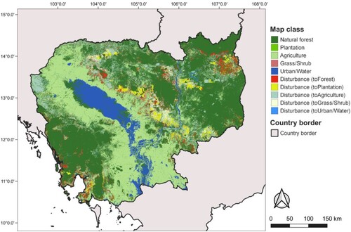
Figure 4. Mapped area of each disturbance type in each year.

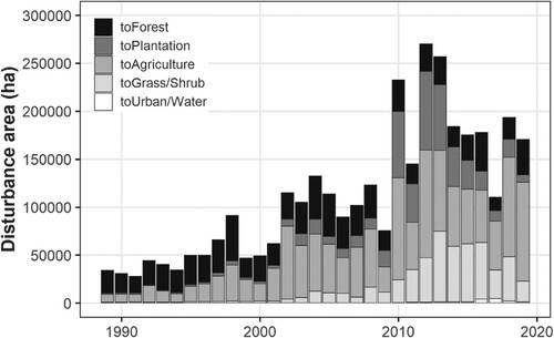
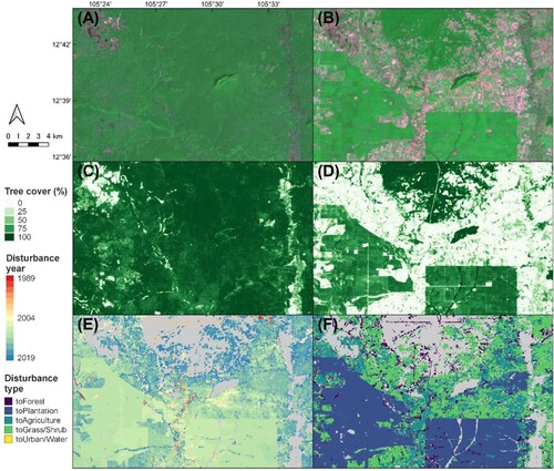
Figure 5. Examples of mapping results for (A) Landsat composite image in 1989, (B) Landsat composite image in 2019, (C) tree canopy cover in 1989, (D) tree canopy cover in 2019, (E) disturbance year from 1989 to 2019, and (F) disturbance types from 1989­ to 2019 in Kampong Thom province (in central Cambodia).

The accuracy assessment showed that the OA of the 10 classes of disturbance types and land cover classification was 78.1% (95% confidence interval: ±2.1%, Table 1). The PA and UA of disturbance classes ranged from 23.7% (±17.8%) to 83.6% (±10.5%) and 68.0% (±10.6%) to 84.0% (±8.4%), respectively. Among the disturbance classes, toAgriculture disturbance occupied the largest area in the error-adjusted estimation of 1.52 million ha (44.0%) and the 95% confidence interval of ± 0.17 million ha followed by toGrass/Shrub (0.78 ± 0.13 million ha, 22.6%) and toPlantation (0.60 ± 0.11 million ha, 17.4%) in 1989–2019. When consolidated to 3 classes, the OA was 87.2% (±1.6%). The PA and UA of the disturbance classes were 77.2% (±4.2%) and 96.8% (±1.8%), respectively, indicating that few commission errors occurred when disturbance classes were aggregated.

Although the disturbance class of the consolidated 3-class classification achieved high accuracies, we found low PA for some disturbance types in the 10-class classification. This result was partially explained by the omission and commission errors of disturbances in deciduous forests. Such errors occurred because low TCC in deciduous forests is confused with other land cover classes and the phenological noise of deciduous forests reduces detection accuracy (Grogan et al. 2015). Furthermore, forest disturbances that occurred at the end of the study period were inherently prone to classification errors since information on the land cover after disturbances was not available. These omissions might be further exacerbated because disturbance detection algorithms that use the entire time series, such as LandTrendr, are prone to errors at the end of time series (Bullock, Woodcock, and Holden 2020a). In this study, toGrass/Shrub indicated disturbance without agriculture or plantation development; however, it would usually take several years after disturbances to detect signs of these land cover changes, leading to low classification accuracies.

Several land cover classes also had low PA and UA in the accuracy assessment of the 10-class classification. Most of the misclassifications of the Plantation class were confused with the Natural forest class. Because the spectral responses of the rubber plantations are usually similar to those of natural forests, this result is not surprising. In addition, the collection of training samples for rubber plantations was sometimes difficult due to spectral similarities, especially when there was no conversion from natural forests to rubber plantations. The possible mislabeling in the visual interpretation might exacerbate estimation accuracies. On the other hand, the forest disturbance (toPlantation) class achieved moderate accuracy. This result might be explained by the use of predictor variables from the LandTrendr temporal segmentation, which reflected the different recovery patterns between natural forests and rubber plantations.

The accuracy assessments in this study might contain the variability of reference sample collection, which was not accounted for. As the previous studies indicated, reference labeling in visual interpretation has a certain degree of variability among different interpreters (Pengra et al. 2020; Stehman et al. 2022). Different interpreters might label different classes to the same reference samples; however, multiple interpreters with quality control protocols would mitigate the bias and precision caused by mislabeling errors (McRoberts et al. 2018). Therefore, it is desirable to include several interpreters and resolve inconsistency among interpreters in visual interpretation (Stehman and Foody 2019). Although the trained interpreter implemented visual interpretation in this study, there might be interpretation errors that were not accounted for, due to the lack of multiple interpreters. Other important uncertainty exists in the visual interpretation of forest degradation. Although the reduction of tree canopy cover after a disturbance was used for determining the forest degradation and recovery in visual interpretation, it was difficult to label parts of samples due to the lack of high-spatial-resolution data, especially for forest disturbances that occurred before 2010. Such forest disturbances were prone to cause misinterpretation. These uncertainties that were not accounted for should be considered to understand the results of this study.

The accuracy of disturbance (i.e. forest loss) detection of the GFC data was lower than that of disturbance type/land cover classification, with the PA and UA of 64.0% (±5.3%) and 79.4% (±5.1%), respectively (Table 2). The mapped disturbance area from 2001 to 2019 was 5.2% larger than forest loss area in the GFC data. Annual comparison achieved an R² of 0.71 and RMSE of 38,187 ha (Figure 6). Although the accuracy of the GFC dataset in a specific country is not always consistent with that of the global scale (Palahí et al. 2021; Bos et al. 2019), the GFC dataset provides a good approximation of forest loss at the country-level (Galiatsatos et al. 2020). The PA and UA of forest loss in the GFC data were lower than those of forest disturbances in the disturbance type/land cover classification; however, the high similarity in trends and area of forest disturbance in this study indicates the plausibility of our mapping approach in Cambodia.

Figure 6. Comparison of mapped annual disturbance area and forest loss area in Hansen et al. (2013).

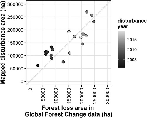
Table 2. Accuracy assessment for forest loss detection in Hansen et al. (2013) using the 3 aggregated classes. PA and UA for each class, and OA are shown with 95% confidence intervals.

Class	PA (%)	UA (%)	OA (%)
Stable forest	83.2 (±3.0)	77.5 (±2.9)	79.8 (±1.9)
Other land cover	82.9 (±2.7)	82.1 (±2.7)
Disturbance (forest loss)	64.0 (±5.3)	79.4 (±5.1)

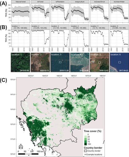
The R² and RMSE for TCC were 0.79 and 19.0%, respectively. The comparison with the existing TCC dataset showed that high similarities were obtained for both the datasets of Hansen et al. (2013) (R² of 0.77 and RMSE of 19.2% for TCC 2000) and Potapov et al. (2019) (R² of 0.86 and 0.85; RMSE of 14.3% and 15.3% for TCC 2000 and 2017, respectively) (Figure 7). The accuracy assessment using the reference samples for TCC achieved the R² and RMSE of 0.44 and 33.9%, respectively, for TCC by Hansen et al. (2013) and R² and RMSE of 0.72 and 22.1%, respectively, for TCC by Potapov et al. (2019). This result indicates that the locally adjusted TCC estimation have higher accuracy compared with these existing datasets. The summary of TCC estimation in natural forest and forest disturbance classes across Cambodia demonstrated the time series variation of TCC estimates (Figure 8). Examples of each disturbance class show relatively stable TCC estimation before disturbance events (Figure 8). The TCC before and after disturbance show different annual variation for the two disturbance classes, in which forests remained as forests after disturbance (Figure S1). Generally, TCC after toPlantation had lower values compared with those in toForest. We assumed that this result was obtained because several years are usually required for rubber plantations to develop a canopy after clearing all vegetation in natural forests (Beckschäfer 2017). The spectral characteristics of young rubber trees are strongly affected by the bare soil and understory vegetation (Chen et al. 2018), which might also cause large variation in TCC after toPlantation.

Figure 7. Comparison of tree canopy cover (TCC) against datasets from Hansen et al. (2013) for 2000 and Potapov et al. (2019) for 2000 and 2017.

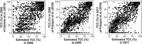
Figure 8. (A) Mean and standard deviation of TCC estimation for stable natural forest and each disturbance type that occurred in 2012 across Cambodia. (B) TCC estimation and the latest high-spatial-resolution data in Google Earth Pro for example locations of stable natural forest and each disturbance type. (C) TCC estimation in 2019 with locations that correspond to examples in (B).

4.2 Mapping deforestation, forest degradation, and recovery

The mapped deforestation, forest degradation, and recovery in 1990–2014 are shown in Figure 9. The OA of classification was 94.4% (±1.1%). Accuracy assessment yielded a relatively higher PA for recovery (72.9%) followed by deforestation (64.7%) and forest degradation (59.1%). The UA was the highest in deforestation (91.6%) followed by forest degradation (74.0%) and recovery (60.8%). Overall, the mapping approach using post-disturbance land covers and TCC provided moderate accuracy. Since the rule-based classification of deforestation, forest degradation, and recovery depended on disturbance classification and TCC estimation, the accuracy obtained in the rule-based classification was largely affected by these two models. Relatively low PA in deforestation stemmed from low PA in disturbance types/land cover classification, especially affected by toGrass/Shrub and toUrban/Water. Large uncertainties of PA and area estimates (i.e. 95% confidence intervals) for small area classes like forest disturbances are also reported in previous studies. To obtain more reliable estimates, the use of a buffer stratum in accuracy assessment might be a viable solution (Olofsson et al. 2020). Although the efficiency of the buffer stratum differs depending on the size of the buffer stratum and the area proportion of the larger stratum, this procedure would be a simple way to reduce estimation uncertainties. The accuracy difference between forest degradation and recovery was also affected by both land cover classification and TCC estimation. In 1990–2014, deforestation, forest degradation, and recovery occupied 64.0%, 22.0%, and 14.0% of the forest disturbance area, respectively (Table 3). In Cambodia, 46.86% of the country was covered with forests in 2018 based on visual interpretation (Ministry of Environment Cambodia 2020). The error-adjusted area of stable forest and disturbance (toForest and toPlantation) in this study (i.e. 45.4%) was similar to this figure, revealing that the automatic mapping approach might be effective for forest monitoring.

Figure 9. Map of deforestation, forest degradation, and recovery across Cambodia, 1990–2014.

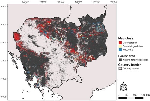
Table 3. Accuracy assessment for deforestation, forest degradation, and recovery. Error-adjusted area, PA and UA for each class, and OA are shown with 95% confidence intervals.

Class	Area (ha)	PA (%)	UA (%)	OA (%)
Stable forest/Other land cover	15,544,240 (±209,142)	99.3 (±0.4)	96.1 (±1.0)	94.4 (±1.1)
Deforestation	1,655,519 (±183,737)	64.7 (±6.8)	91.6 (±5.2)
Forest degradation	569,231 (±120,699)	59.1 (±11.7)	74.0 (±10.8)
Recovery	361,825 (±100,656)	72.9 (±14.7)	60.8 (±12.6)

The TCC relative to the original states before disturbance could distinguish forest degradation and recovery in forests with different original TCC levels. In Cambodia, TCC is high in evergreen and semi-evergreen forests but low in deciduous forests (Potapov et al. 2019). In areas with such different forest types, it is difficult to assess forest degradation and recovery using a fixed TCC threshold. In this regard, we provided a better mapping approach for different forest types. In addition, the approach here can be changed to suit different study objectives. Forest degradation/recovery in this study included rubber plantations, which were treated as forests. However, natural forests converted to plantations can be degraded in terms of environmental services, as reported in (Scheidel and Work 2018). Our approach is applicable to different definitions of forest degradation/recovery because the estimated disturbance type and TCC can be adjusted to the desired definitions.

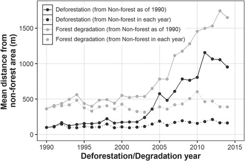
Distance from the non-forest area in each year was higher for forest degradation (mean: 424.5 m) compared with deforestation (mean: 156.4 m). In each year, 72.2% of forest degradation and 94.4% of deforestation areas were located within 500 m from a non-forest area. The distance from non-forest in each year was stable through time for both deforestation and forest degradation (Figure 10). Because the distance from roads and other non-forest areas is an important indicator for forest loss in the tropics (Mon et al. 2012; Ehara et al. 2021; Oliveira et al. 2007), it was not surprising that disturbance frequently occurred near the forest edge (i.e. near non-forest). Interestingly, however, the distance from non-forest as of 1990 increased from the 2000s both for deforestation and forest degradation (Figure 10). This result indicated that the disturbance areas were gradually moving into places previously covered with forests, in contrast to before the 2000s. Deforestation in Cambodia has been accelerated by large-scale industrial development and the expansion of agricultural land under rapid economic growth (Tsujino, Kajisa, and Yumoto 2019). The increased distance trend seems to reflect such deforestation and forest degradation patterns, which were not apparent before economic growth.

Figure 10. Temporal trends of mean distance from non-forest area in each year and non-forest area as of 1990.

5. Conclusions

We developed an approach for mapping annual deforestation, forest degradation, and recovery using disturbance types/land cover classification and TCC estimation from Landsat time series in Cambodia. Overall, rule-based classification of deforestation, forest degradation, and recovery yielded a moderate accuracy. The mapped deforestation, forest degradation, and recovery provided an understanding of the spatial and temporal patterns of forest changes across the country. The mapped disturbance types and TCC were helpful to characterize post-disturbance conditions. In Cambodia, the government has mapped land use/land cover change based on manual interpretation using the segmentation of satellite images across the country (Ministry of Environment Cambodia 2020). Although such an approach might eliminate errors caused by automated classification algorithms, the consistent and automatic mapping approaches in the current study can assist with more frequent (e.g. annual) monitoring of land cover changes. While the definitions of forest degradation/recovery might differ according to research objectives, the combinations of disturbance types and tree canopy cover estimates in this study can be flexibly modified to suit specific requirements. Thus, our approach is potentially applicable for other study sites over large areas. Although the use of RF models in our study can improve the prediction accuracy, one limitation of the approach is the requirement of sufficient training samples to develop valid prediction models for mapping disturbance type/land cover classes and TCC. As the performance of RF models is affected by the derivation of variables, the investigations on effective predictor variables might reduce training samples that achieve high prediction accuracy.

Acknowledgements

We thank Leonie Seabrook, PhD, from Edanz (https://jp.edanz.com/ac) for editing a draft of this manuscript. We thank four anonymous reviewers for their constructive comments.

Disclaimer statement

The views and interpretation of this study are those of the authors and do not necessarily reflect the views and opinions of any institution.

Disclosure statement

No potential conflict of interest was reported by the author(s).

Data availability

The data supporting this study and code for analysis will be provided by the corresponding author upon reasonable request.

Additional information

Funding

This study was funded by JSPS grant number [JP19H04339].

References

- Arévalo, Paulo, Pontus Olofsson, and Curtis E. Woodcock. 2020. “Continuous Monitoring of Land Change Activities and Post-Disturbance Dynamics from Landsat Time Series: A Test Methodology for REDD+ Reporting.” Remote Sensing of Environment 238 (1): 111051. doi:10.1016/J.RSE.2019.01.013.
- Aryal, Raja Ram, Crystal Wespestad, Robert Kennedy, John Dilger, Karen Dyson, Eric Bullock, Nishanta Khanal, et al. 2021. “Lessons Learned While Implementing a Time-Series Approach to Forest Canopy Disturbance Detection in Nepal.” Remote Sensing 13 (14): 2666. doi:10.3390/RS13142666.
- Asner, G. P., D. E. Knapp, E. N. Broadbent, P. J. C. Oliveira, M. Keller, and J. N. Silva. 2005. “Ecology: Selective Logging in the Brazilian Amazon.” Science 310 (5747): 480–482. doi:10.1126/science.1118051.
- Baccini, A., W. Walker, L. Carvalho, M. Farina, D. Sulla-Menashe, and R. A. Houghton. 2017. “Tropical Forests Are a Net Carbon Source Based on Aboveground Measurements of Gain and Loss.” Science 358 (6360): 230–234. doi:10.1126/science.aam5962.
- Beckschäfer, Philip. 2017. “Obtaining Rubber Plantation Age Information from Very Dense Landsat TM & ETM+ Time Series Data and Pixel-Based Image Compositing.” Remote Sensing of Environment 196: 89–100. doi:10.1016/j.rse.2017.04.003.
- Bos, Astrid B., Veronique De Sy, Amy E. Duchelle, Martin Herold, Christopher Martius, and Nandin-Erdene Tsendbazar. 2019. “Global Data and Tools for Local Forest Cover Loss and REDD+ Performance Assessment: Accuracy, Uncertainty, Complementarity and Impact.” International Journal of Applied Earth Observation and Geoinformation 80 (August): 295–311. doi:10.1016/J.JAG.2019.04.004.
- Bullock, Eric L., Curtis E. Woodcock, and Christopher E. Holden. 2020a. “Improved Change Monitoring Using an Ensemble of Time Series Algorithms.” Remote Sensing of Environment 238 (May): 111165. doi:10.1016/J.RSE.2019.04.018.
- Bullock, Eric L., Curtis E. Woodcock, and Pontus Olofsson. 2020b. “Monitoring Tropical Forest Degradation Using Spectral Unmixing and Landsat Time Series Analysis.” Remote Sensing of Environment 238(November): 110968. doi:10.1016/J.RSE.2018.11.011.
- Chen, Gang, Jean-Claude Thill, Sutee Anantsuksomsri, Nij Tontisirin, and Ran Tao. 2018. “Stand Age Estimation of Rubber (Hevea Brasiliensis) Plantations Using an Integrated Pixel- and Object-Based Tree Growth Model and Annual Landsat Time Series.” ISPRS Journal of Photogrammetry and Remote Sensing 144 (October): 94–104. doi:10.1016/J.ISPRSJPRS.2018.07.003.
- Crist, E. P. 1985. “A TM Tasseled Cap Equivalent Transformation for Reflectance Factor Data.” Remote Sensing of Environment 17 (3): 301–306. doi:10.1016/0034-4257(85)90102-6.
- Davis, Kyle Frankel, Kailiang Yu, Maria Cristina Rulli, Lonn Pichdara, and Paolo D’Odorico. 2015. “Accelerated Deforestation Driven by Large-Scale Land Acquisitions in Cambodia.” Nature Geoscience 8 (10): 772–775. doi:10.1038/ngeo2540.
- de Bem, Pablo Pozzobon, Osmar Abílio de Carvalho Júnior, Osmar Luiz Ferreira de Carvalho, Roberto Arnaldo Trancoso Gomes, and Renato Fontes Guimarães. 2020. “Performance Analysis of Deep Convolutional Autoencoders with Different Patch Sizes for Change Detection from Burnt Areas.” Remote Sensing 12 (16): 2576. doi:10.3390/rs12162576.
- De Marzo, Teresa, Dirk Pflugmacher, Matthias Baumann, Eric F. Lambin, Ignacio Gasparri, and Tobias Kuemmerle. 2021. “Characterizing Forest Disturbances Across the Argentine Dry Chaco Based on Landsat Time Series.” International Journal of Applied Earth Observation and Geoinformation 98 (June): 102310. doi:10.1016/j.jag.2021.102310.
- Duarte, Efraín, Juan A. Barrera, Francis Dube, Fabio Casco, Alexander J. Hernández, and Erick Zagal. 2020. “Monitoring Approach for Tropical Coniferous Forest Degradation Using Remote Sensing and Field Data.” Remote Sensing 12 (16): 2531. doi:10.3390/rs12162531.
- Dupuis, Chloé, Philippe Lejeune, Adrien Michez, and Adeline Fayolle. 2020. “How Can Remote Sensing Help Monitor Tropical Moist Forest Degradation?—A Systematic Review.” Remote Sensing 12 (7): 1087. doi:10.3390/RS12071087.
- Ehara, Makoto, Hideki Saito, Tetsuya Michinaka, Yasumasa Hirata, Chivin Leng, Mitsuo Matsumoto, and Carlos Riano. 2021. “Allocating the REDD+ National Baseline to Local Projects: A Case Study of Cambodia.” Forest Policy and Economics 129 (August): 02474. doi:10.1016/j.forpol.2021.102474.
- Estoque, Ronald C., Brian Alan Johnson, Yan Gao, Rajarshi DasGupta, Makoto Ooba, Takuya Togawa, Yasuaki Hijioka, et al. 2021. “Remotely Sensed Tree Canopy Cover–Based Indicators for Monitoring Global Sustainability and Environmental Initiatives.” Environmental Research Letters 16 (4): 44047. doi:10.1088/1748-9326/abe5d9.
- FAO. 2020. Global Forest Resources Assessment 2020. Rome: UN Food and Agriculture Organization. doi:10.4060/ca9825en.
- FAO. 2001. Global Forest Resources Assessment 2000. Rome: UN Food and Agriculture Organization.
- Farr, Tom G., Paul A. Rosen, Edward Caro, Robert Crippen, Riley Duren, Scott Hensley, Michael Kobrick, et al. 2007. “The Shuttle Radar Topography Mission.” Reviews of Geophysics 45: RG2004. doi:10.1029/2005RG000183.
- Finer, Matt, Sidney Novoa, J. Weisse, Rachael Petersen, Tamia Souto, Forest Stearns, and Raúl García Martinez. 2018. “Combating Deforestation: From Satellite to Intervention.” Science 360 (6395): 1303–1305. doi:10.1126/science.aat1203.
- Fox, Jefferson, and Jean-Christophe Castella. 2013. “Expansion of Rubber (Hevea Brasiliensis) in Mainland Southeast Asia: What Are the Prospects for Smallholders?” Journal of Peasant Studies 40 (1): 155–170. doi:10.1080/03066150.2012.750605.
- Franklin, Steven E., Oumer S. Ahmed, Michael A. Wulder, Joanne C. White, Txomin Hermosilla, and Nicholas C. Coops. 2015. “Large Area Mapping of Annual Land Cover Dynamics Using Multitemporal Change Detection and Classification of Landsat Time Series Data.” Canadian Journal of Remote Sensing 41 (4): 293–314. doi:10.1080/07038992.2015.1089401.
- Galiatsatos, Nikolaos, Daniel N.M. Donoghue, Pete Watt, Pradeepa Bholanath, Jeffrey Pickering, Matthew C. Hansen, and Abu R.J. Mahmood. 2020. “An Assessment of Global Forest Change Datasets for National Forest Monitoring and Reporting.” Remote Sensing 12 (11): 1790. doi:10.3390/RS12111790.
- Gao, Yan, Margaret Skutsch, Jaime Paneque-Gálvez, and Adrian Ghilardi. 2020. “Remote Sensing of Forest Degradation: A Review.” Environmental Research Letters 15 (10): 103001. doi:10.1088/1748-9326/abaad7.
- Geist, H. J., and E. F. Lambin. 2002. “Proximate Causes and Underlying Driving Forces of Tropical Deforestation.” BioScience 52 (2): 143–150. doi:10.1641/0006-3568(2002)052[0143:PCAUDF]2.0.CO;2.
- Global Forest Observations Initiative. 2020. Integration of Remote-Sensing and Ground-Based Observations for Estimation of Emissions and Removals of Greenhouse Gases in Forests: Methods and Guidance from the Global Forest Observations Initiative, Edition 3.0. Rome: UN Food and Agriculture Organization.
- Gorelick, Noel, Matt Hancher, Mike Dixon, Simon Ilyushchenko, David Thau, and Rebecca Moore. 2017. “Google Earth Engine: Planetary-Scale Geospatial Analysis for Everyone.” Remote Sensing of Environment 202: 18–27. doi:10.1016/j.rse.2017.06.031.
- Grassi, Giacomo, Alessandro Cescatti, and Guido Ceccherini. 2021. “JRC Study on Harvested Forest Area: Resolving Key Misunderstandings.” IForest 14 (3): 231–235. doi:10.3832/ifor0059-014.
- Grogan, Kenneth, Dirk Pflugmacher, Patrick Hostert, Robert Kennedy, and Rasmus Fensholt. 2015. “Cross-Border Forest Disturbance and the Role of Natural Rubber in Mainland Southeast Asia Using Annual Landsat Time Series.” Remote Sensing of Environment 169 (April): 438–453. doi:10.1016/j.rse.2015.03.001.
- Grogan, Kenneth, Dirk Pflugmacher, Patrick Hostert, Ole Mertz, and Rasmus Fensholt. 2018. “Unravelling the Link Between Global Rubber Price and Tropical Deforestation in Cambodia.” Nature Plants 5 (December): 47–53. doi:10.1038/s41477-018-0325-4.
- Hamunyela, Eliakim, Patric Brandt, Deo Shirima, Ha Thi Thanh Do, Martin Herold, and Rosa Maria Roman-Cuesta. 2020. “Space-Time Detection of Deforestation, Forest Degradation and Regeneration in Montane Forests of Eastern Tanzania.” International Journal of Applied Earth Observation and Geoinformation 88 (June): 102063. doi:10.1016/J.JAG.2020.102063.
- Hamunyela, Eliakim, Jan Verbesselt, Sytze de Bruin, and Martin Herold. 2016. “Monitoring Deforestation at Sub-Annual Scales as Extreme Events in Landsat Data Cubes.” Remote Sensing 8 (8): 651. doi:10.3390/rs8080651.
- Hansen, M. C., P. V. Potapov, R. Moore, M. Hancher, S. A. Turubanova, A. Tyukavina, D. Thau, et al. 2013. “High-Resolution Global Maps of 21st-Century Forest Cover Change.” Science 342 (2013): 850–853. doi:10.1126/science.1244693.
- Hethcoat, Matthew, Joao Carreiras, David Edwards, Robert Bryant, Carlos Peres, and Shaun Quegan. 2020. “Mapping Pervasive Selective Logging in the South-West Brazilian Amazon 2000–2019.” Environmental Research Letters 15 (9): 094057. doi:10.1088/1748-9326/aba3a4.
- Hijmans, Robert J. 2020. “Raster: Geographic Data Analysis and Modeling.” https://cran.r-project.org/web/packages/raster/.
- Hosonuma, Noriko, Martin Herold, Veronique De Sy, Ruth S De Fries, Maria Brockhaus, Louis Verchot, Arild Angelsen, and Erika Romijn. 2012. “An Assessment of Deforestation and Forest Degradation Drivers in Developing Countries.” Environmental Research Letters 7 (4): 044009. doi:10.1088/1748-9326/7/4/044009.
- Kennedy, R. E., Z. Yang, and W. B. Cohen. 2010. “Detecting Trends in Forest Disturbance and Recovery Using Yearly Landsat Time Series: 1. LandTrendr – Temporal Segmentation Algorithms.” Remote Sensing of Environment 114 (12): 2897–2910. doi:10.1016/j.rse.2010.07.008.
- Key, Carl H, and Nathan C Benson. 2006. Landscape Assessment (LA): Sampling and Analysis Methods. USDA Forest Service General Technical Report RMS-GTR-164-CD, Fort Collins, CO.
- Kong, Rada, Jean Christophe Diepart, Jean Christophe Castella, Guillaume Lestrelin, Florent Tivet, Elisa Belmain, and Agnès Bégué. 2019. “Understanding the Drivers of Deforestation and Agricultural Transformations in the Northwestern Uplands of Cambodia.” Applied Geography 102 (January): 84–98. doi:10.1016/j.apgeog.2018.12.006.
- Kuhn, Max. 2008. “Building Predictive Models in R Using the caret Package.” Journal of Statistical Software 28 (5). doi:10.18637/jss.v028.i05.
- Lewis, Simon L., David P. Edwards, and David Galbraith. 2015. “Increasing Human Dominance of Tropical Forests.” Science. doi:10.1126/science.aaa9932.
- Liaw, Andy, and Matthew Wiener. 2002. “Classification and Regression by RandomForest.” R News 2 (3): 18–22.
- Magliocca, Nicholas R, Quy Van Khuc, Ariane de Bremond, and Evan A Ellicott. 2020. “Direct and Indirect Land-Use Change Caused by Large-Scale Land Acquisitions in Cambodia.” Environmental Research Letters 15 (2): 024010. doi:10.1088/1748-9326/ab6397.
- Masek, Jeffrey G, Eric F Vermote, Nazmi E Saleous, Robert Wolfe, Forrest G Hall, Karl F Huemmrich, Feng Gao, Jonathan Kutler, and Teng Kui Lim. 2006. “A Landsat Surface Reflectance Dataset for North America, 1990-2000.” IEEE Geoscience and Remote Sensing Letters 3 (1): 68–72. doi:10.1109/LGRS.2005.857030.
- Matricardi, Eraldo A T, David L Skole, Marcos A Pedlowski, Walter Chomentowski, and Luis Claudio Fernandes. 2010. “Assessment of Tropical Forest Degradation by Selective Logging and Fire Using Landsat Imagery.” Remote Sensing of Environment 114 (5): 1117–1129. doi:10.1016/j.rse.2010.01.001.
- McRoberts, Ronald E., Stephen V. Stehman, Greg C. Liknes, Erik Næsset, Christophe Sannier, and Brian F. Walters. 2018. “The Effects of Imperfect Reference Data on Remote Sensing-Assisted Estimators of Land Cover Class Proportions.” ISPRS Journal of Photogrammetry and Remote Sensing 142 (August): 292–300. doi:10.1016/J.ISPRSJPRS.2018.06.002.
- Miettinen, Jukka, Hans-Jürgen Stibig, and Frédéric Achard. 2014. “Remote Sensing of Forest Degradation in Southeast Asia—Aiming for a Regional View Through 5–30 m Satellite Data.” Global Ecology and Conservation 2 (August): 24–36. doi:10.1016/j.gecco.2014.07.007.
- Ministry of Environment Cambodia. 2020. Cambodia Forest Cover 2018. Phnom Penh.
- Mitchard, Edward T. A. 2018. “The Tropical Forest Carbon Cycle and Climate Change.” Nature 559 (7715): 527–534. doi:10.1038/s41586-018-0300-2.
- Mitchell, Anthea L., Ake Rosenqvist, and Brice Mora. 2017. “Current Remote Sensing Approaches to Monitoring Forest Degradation in Support of Countries Measurement, Reporting and Verification (MRV) Systems for REDD+.” Carbon Balance and Management 12 (1): 9. doi:10.1186/s13021-017-0078-9.
- Modica, Giuseppe, Angelo Merlino, Francesco Solano, and Roberto Mercurio. 2015. “An index for the assessment of degraded Mediterranean forest ecosystems.” Forest Systems 24 (3): e037. doi: 10.5424/fs/2015243-07855.
- Mon, Myat Su, Nobuya Mizoue, Naing Zaw Htun, Tsuyoshi Kajisa, and Shigejiro Yoshida. 2012. “Factors Affecting Deforestation and Forest Degradation in Selectively Logged Production Forest: A Case Study in Myanmar.” Forest Ecology and Management 267: 190–198. doi:10.1016/j.foreco.2011.11.036.
- Morales-Barquero, Lucia, Margaret Skutsch, Enrique J Jardel-Peláez, Adrian Ghilardi, Christoph Kleinn, and John R Healey. 2014. “Operationalizing the Definition of Forest Degradation for REDD, with Application to Mexico.” Forests 5 (7): 1653–1681.
- Murillo-Sandoval, Paulo J, Thomas Hilker, Meg A Krawchuk, and Jamon Van Den Hoek. 2018. “Detecting and Attributing Drivers of Forest Disturbance in the Colombian Andes Using Landsat Time-Series.” Forests 9 (5): 269.
- Oliveira, Paulo J. C., Gregory P. Asner, David E. Knapp, Angélica Almeyda, Ricardo Galván-Gildemeister, Sam Keene, Rebecca F. Raybin, and Richard C. Smith. 2007. “Land-Use Allocation Protects the Peruvian Amazon.” Science 317 (5842): 1233–1236. doi:10.1126/SCIENCE.1146324.
- Olofsson, Pontus, Paulo Arévalo, Andres B. Espejo, Carly Green, Erik Lindquist, Ronald E. McRoberts, and María J. Sanz. 2020. “Mitigating the Effects of Omission Errors on Area and Area Change Estimates.” Remote Sensing of Environment 236 (January): 111492. doi:10.1016/J.RSE.2019.111492.
- Olofsson, Pontus, Giles M Foody, Martin Herold, Stephen V Stehman, Curtis E Woodcock, and Michael A Wulder. 2014. “Good Practices for Estimating Area and Assessing Accuracy of Land Change.” Remote Sensing of Environment 148: 42–57. doi:10.1016/j.rse.2014.02.015.
- Ota, Tetsuji, Pichdara Lonn, and Nobuya Mizoue. 2020. “A Country Scale Analysis Revealed Effective Forest Policy Affecting Forest Cover Changes in Cambodia.” Land Use Policy 95 (June): 104597. doi:10.1016/j.landusepol.2020.104597.
- Palahí, Marc, Rubén Valbuena, Cornelius Senf, Nezha Acil, Thomas A.M. Pugh, Jonathan Sadler, Rupert Seidl, et al. 2021. “Concerns About Reported Harvests in European Forests.” Nature Research. doi:10.1038/s41586-021-03292-x.
- Pan, Yude, Richard A Birdsey, Jingyun Fang, Richard Houghton, Pekka E Kauppi, Werner A Kurz, Oliver L Phillips, et al. 2011. “A Large and Persistent Carbon Sink in the World’s Forests.” Science 333 (6045): 988–993. doi:10.1126/science.1201609.
- Pengra, Bruce W., Stephen V. Stehman, Josephine A. Horton, Daryn J. Dockter, Todd A. Schroeder, Zhiqiang Yang, Warren B. Cohen, Sean P. Healey, and Thomas R. Loveland. 2020. “Quality Control and Assessment of Interpreter Consistency of Annual Land Cover Reference Data in an Operational National Monitoring Program.” Remote Sensing of Environment 238 (June): 111261. doi:10.1016/J.RSE.2019.111261.
- Phiri, Darius, Matamyo Simwanda, Serajis Salekin, Vincent R. Nyirenda, Yuji Murayama, and Manjula Ranagalage. 2020. “Sentinel-2 Data for Land Cover/Use Mapping: A Review.” Remote Sensing 12 (14): 2291. doi:10.3390/rs12142291.
- Potapov, P., A. Tyukavina, S. Turubanova, Y. Talero, A. Hernandez-Serna, M. C. Hansen, D. Saah, et al. 2019. “Annual Continuous Fields of Woody Vegetation Structure in the Lower Mekong Region from 2000-2017 Landsat Time-Series.” Remote Sensing of Environment 232 (October): 111278. doi:10.1016/J.RSE.2019.111278.
- Raši, Rastislav, Catherine Bodart, Hans Jürgen Stibig, Hugh Eva, René Beuchle, S. Carboni, Dario Simonetti, and F. Achard. 2011. “An Automated Approach for Segmenting and Classifying a Large Sample of Multi-Date Landsat Imagery for Pan-Tropical Forest Monitoring.” Remote Sensing of Environment 115: 3659–3669. doi:10.1016/j.rse.2011.09.004.
- R Core Team. 2021. "R: A Language and Environment for Statistical Computing." R Foundation for Statistical Computing. Vienna, Austria. https://www.r-project.org/
- Reygadas, Yunuen, Stephanie Spera, Valerie Galati, David S Salisbury, Sonaira Silva, and Sidney Novoa. 2021. “Mapping Forest Disturbances Across the Southwestern Amazon: Tradeoffs Between Open-Source, Landsat-Based Algorithms.” Environmental Research Communications 3 (9): 091001. doi:10.1088/2515-7620/AC2210.
- Roy, D. P., V. Kovalskyy, H. K. Zhang, E. F. Vermote, L. Yan, S. S. Kumar, and A. Egorov. 2016. “Characterization of Landsat-7 to Landsat-8 Reflective Wavelength and Normalized Difference Vegetation Index Continuity.” Remote Sensing of Environment 185 (November): 57–70. doi:10.1016/j.rse.2015.12.024.
- Sannier, Christophe, Louis-Vincent Fichet, and Etienne Massard K Makaga. 2014. “Using the Regression Estimator with Landsat Data to Estimate Proportion Forest Cover and Net Proportion Deforestation in Gabon.” Remote Sensing of Environment 151 (August): 138–148. doi:10.1016/J.RSE.2013.09.015.
- Schaafsma, M., S. Morse-Jones, P. Posen, R. D. Swetnam, A. Balmford, I. J. Bateman, N. D. Burgess, et al. 2014. “The Importance of Local Forest Benefits: Economic Valuation of Non-Timber Forest Products in the Eastern Arc Mountains in Tanzania.” Global Environmental Change 24 (1): 295–305. doi:10.1016/j.gloenvcha.2013.08.018.
- Scheidel, Arnim, and Courtney Work. 2018. “Forest Plantations and Climate Change Discourses: New Powers of ‘Green’ Grabbing in Cambodia.” Land Use Policy 77 (September): 9–18. doi:10.1016/j.landusepol.2018.04.057.
- Shimizu, Katsuto, Oumer S. Ahmed, Raul Ponce-Hernandez, Tetsuji Ota, Zar Chi Win, Nobuya Mizoue, and Shigejiro Yoshida. 2017. “Attribution of Disturbance Agents to Forest Change Using a Landsat Time Series in Tropical Seasonal Forests in the Bago Mountains, Myanmar.” Forests 8 (6): 218. doi:10.3390/F8060218.
- Shimizu, Katsuto, Tetsuji Ota, and Nobuya Mizoue. 2020. “Accuracy Assessments of Local and Global Forest Change Data to Estimate Annual Disturbances in Temperate Forests.” Remote Sensing 12 (15): 2438. doi:10.3390/RS12152438.
- Shimizu, Katsuto, Tetsuji Ota, Nobuya Mizoue, and Shigejiro Yoshida. 2019. “A Comprehensive Evaluation of Disturbance Agent Classification Approaches: Strengths of Ensemble Classification, Multiple Indices, Spatio-Temporal Variables, and Direct Prediction.” ISPRS Journal of Photogrammetry and Remote Sensing 158 (December): 99–112. doi:10.1016/J.ISPRSJPRS.2019.10.004.
- Shimizu, Katsuto, and Hideki Saito. 2021. “Country-Wide Mapping of Harvest Areas and Post-Harvest Forest Recovery Using Landsat Time Series Data in Japan.” International Journal of Applied Earth Observation and Geoinformation 104 (December): 102555. doi:10.1016/J.JAG.2021.102555.
- Souza, C. M., J. V. Siqueira, M. H. Sales, A. V. Fonseca, J. G. Ribeiro, I. Numata, M. A. Cochrane, C. P. Barber, D. A. Roberts, and J. Barlow. 2013. “Ten-Year Landsat Classification of Deforestation and Forest Degradation in the Brazilian Amazon.” Remote Sensing 5: 5493–5513. doi:10.3390/rs5115493.
- Stehman, Stephen V. 2014. “Estimating Area and Map Accuracy for Stratified Random Sampling When the Strata Are Different from the Map Classes.” International Journal of Remote Sensing 35 (13): 4923–4939. doi:10.1080/01431161.2014.930207.
- Stehman, Stephen V., and Giles M. Foody. 2019. “Key Issues in Rigorous Accuracy Assessment of Land Cover Products.” Remote Sensing of Environment 231 (September): 111199. doi:10.1016/J.RSE.2019.05.018.
- Stehman, Stephen V., John Mousoupetros, Ronald E. McRoberts, Erik Næsset, Bruce W. Pengra, Dingfan Xing, and Josephine A. Horton. 2022. “Incorporating Interpreter Variability Into Estimation of the Total Variance of Land Cover Area Estimates Under Simple Random Sampling.” Remote Sensing of Environment 269 (February): 112806. doi:10.1016/J.RSE.2021.112806.
- Tang, Xiaojing, Lucy R Hutyra, Paulo Arévalo, Alessandro Baccini, Curtis E Woodcock, and Pontus Olofsson. 2020. “Spatiotemporal Tracking of Carbon Emissions and Uptake Using Time Series Analysis of Landsat Data: A Spatially Explicit Carbon Bookkeeping Model.” Science of The Total Environment 720 (June): 137409. doi:10.1016/j.scitotenv.2020.137409.
- Tsujino, R., T. Kajisa, and T. Yumoto. 2019. “Causes and History of Forest Loss in Cambodia.” International Forestry Review 21 (3): 372–384. doi:10.1505/146554819827293178.
- Vancutsem, C., F. Achard, J.-F. Pekel, G. Vieilledent, S. Carboni, D. Simonetti, J. Gallego, L. E. O. C. Aragão, and R. Nasi. 2021. “Long-Term (1990–2019) Monitoring of Forest Cover Changes in the Humid Tropics.” Science Advances 7 (10): eabe1603. doi:10.1126/sciadv.abe1603.
- Vásquez-Grandón, Angélica, Pablo Donoso, Víctor Gerding, Angélica Vásquez-Grandón, Pablo J. Donoso, and Víctor Gerding. 2018. “Forest Degradation: When Is a Forest Degraded?” Forests 9 (11): 726. doi:10.3390/F9110726.
- Vermote, Eric, Chris Justice, Martin Claverie, and Belen Franch. 2016. “Preliminary Analysis of the Performance of the Landsat 8/OLI Land Surface Reflectance Product.” Remote Sensing of Environment 185 (November): 46–56. doi:10.1016/j.rse.2016.04.008.
- Wu, Biyun, Xiang Meng, Qiaolin Ye, Ram P Sharma, Guangshuang Duan, Yuancai Lei, and Liyong Fu. 2020. “Method of Estimating Degraded Forest Area: Cases from Dominant Tree Species from Guangdong and Tibet in China.” Forests 11 (9): 930. doi:10.3390/f11090930.
- Wulder, Michael A., Thomas Hilker, Joanne C. White, Nicholas C. Coops, Jeffrey G. Masek, Dirk Pflugmacher, and Yves Crevier. 2015. “Virtual Constellations for Global Terrestrial Monitoring.” Remote Sensing of Environment 170 (December): 62–76. doi:10.1016/j.rse.2015.09.001.
- Xu, Liang, Sassan S. Saatchi, Yan Yang, Yifan Yu, Julia Pongratz, A. Anthony Bloom, Kevin Bowman, et al. 2021. “Changes in Global Terrestrial Live Biomass Over the 21st Century.” Science Advances 7 (27): eabe9829. doi:10.1126/sciadv.abe9829.
- Zanaga, Daniele, Ruben Van De Kerchove, Wanda De Keersmaecker, Niels Souverijns, Carsten Brockmann, Ralf Quast, Jan Wevers, et al. 2021. “ESA WorldCover 10 m 2020 V100.” doi:10.5281/ZENODO.5571936.
- Zhu, Zhe, Shixiong Wang, and Curtis E. Woodcock. 2015. “Improvement and Expansion of the Fmask Algorithm: Cloud, Cloud Shadow, and Snow Detection for Landsats 4–7, 8, and Sentinel 2 Images.” Remote Sensing of Environment 159 (March): 269–277. doi:10.1016/j.rse.2014.12.014.
- Zhu, Zhe, and C. E. Woodcock. 2012. “Object-Based Cloud and Cloud Shadow Detection in Landsat Imagery.” Remote Sensing of Environment 118: 83–94. doi:10.1016/j.rse.2011.10.028.
- Zhuravleva, I., S. Turubanova, P. Potapov, M. Hansen, A. Tyukavina, S. Minnemeyer, N. Laporte, S. Goetz, F. Verbelen, and C. Thies. 2013. “Satellite-Based Primary Forest Degradation Assessment in the Democratic Republic of the Congo, 2000–2010.” Environmental Research Letters 8 (2): 024034. doi:10.1088/1748-9326/8/2/024034.