Evaluation of neural network models for landslide susceptibility assessment

ABSTRACT

Identifying and assessing the disaster risk of landslide-prone regions is very critical for disaster prevention and mitigation. Owning to their special advantages, neural network algorithms have been widely used for landslide susceptibility mapping (LSM) in recent decades. In the present study, three advanced neural network models popularly used in relevant studies, i.e. artificial neural network (ANN), one dimensional convolutional neural network (1D CNN) and recurrent neural network (RNN), were evaluated and compared for LSM practice over the Qingchuan County, Sichuan province, China. Extensive experimental results demonstrated satisfactory performances of these three neural network models in accurately predicting susceptible regions. Specifically, ANN and 1D CNN models yielded quite consistent LSM results but slightly differed from those of RNN model spatially. Nevertheless, accuracy evaluations revealed that the RNN model outperformed the other two models both qualitatively and quantitatively but its complexity was relatively high. Experiments concerning training hyper-parameters on the performance of neural network models for LSM suggested that relatively small batch size values with Tanh activation function and SGD optimizer are essential to improve the performance of neural network models for LSM, which may provide a thread to help those who apply these advanced algorithms to improve their efficiency.

KEYWORDS:

• Deep learning
• landslide
• data-driven
• GIS
• Sichuan

1. Introduction

Landslides are a ubiquitous natural hazard that seriously threatens the safety of people’s lives and property as well as human wellbeing alike and will occur more frequently in the future under a changing climate context in mountainous regions in China as well as worldwide (Froude and Petley 2018; Gariano and Guzzetti 2016; Pham et al. 2020). Landslide is a complex and synthetic geographical phenomenon (Yi and Zhang 2020), which describes a wide variety of surface processes (Hungr, Leroueil, and Picarelli 2014; Varnes 1978), including block slide, debris flow and rock fall. Its occurrence and expansion are all affected by various factors, including conditioning factors (topography, geology, etc.) and triggering factors (rainfall, earthquakes, etc.) (Guzzetti et al. 2005). Consequently, landslide susceptibility mapping (LSM), defined as the spatial probability of landslides occurring in a region under the local geo-environmental conditions (Reichenbach et al. 2018), is strongly recommended as a critical step for disaster mitigation and risk management, as well as land planning (Fell et al. 2008). However, due to the complexity of landslide formation (Cruden and Varnes 1996), generating a reliable and accurate landslide susceptibility map yet remains a challenging technique in practice.

In the past decades, various approaches have been developed to assess landslide susceptibility, among which knowledge-based and data-driven approaches were the most popular (Reichenbach et al. 2018; Thi Ngo et al. 2021). Knowledge-based approaches are mainly based on subjective decision rules by relevant experts (Dai and Lee 2002), the frequently used methods include analytical hierarchy process (AHP) (Mansouri Daneshvar 2014; Yi et al. 2019) and fuzzy logic (Zhu et al. 2014). However, subjectivity and uncertainty in their rules of decision making were argued always on the requirement of the guidance of experienced experts to produce satisfactory results. With the advancement of Earth observations, data-driven approaches, including statistical methods and machine learning models, were developed rapidly in LSM for its advantages in focusing on mining the data itself compared with knowledge-based approaches, such as support vector machine (SVM) (Xu et al. 2012), artificial neural network (ANN) (Abbaszadeh Shahri et al. 2019; Gorsevski et al. 2016) and random forest (RF) (Catani et al. 2013; Fan et al. 2021; He, Wang, and Liu 2021). Based on the high-quality spatial data, data-driven approaches are capable of objectively learning and analyzing the complex relationship between landslides and environmental factors. Nevertheless, owning to the different data mining capabilities of the models adopted, results generated by different data-driven methods still vary greatly. For instance, Nsengiyumva et al. (2019) compared the models of weights of evidence, logistic regression, frequency ratio and statistical index adopted in LSM, which proved the effectiveness of weights of evidence. Ali et al. (2021) generated the LSMs by using several machine learning methods, implying the effectiveness of the RF classifier. Moreover, integrated approaches for LSM were also proposed, such as integration of AHP and ANN (Jena et al. 2019), integration of certainty factor and ANN (Dou et al. 2015) and other ensemble methods (Hong et al. 2018). Meanwhile, more robust and novel LSM algorithms have also been explored.

In recent decades, the deep learning technique with its powerful feature extraction capability got tremendous development in image-related tasks (LeCun, Bengio, and Hinton 2015; Wu et al. 2021). Attempts to apply deep learning algorithms to analyze the complex relationship between landslides and environmental factors become research hotspots in recent years (Hua et al. 2021; Lv et al. 2022; Wang, Fang, and Hong 2019). Unlike the traditional machine learning algorithms, the deeper the model structure of deep learning algorithms is, theoretically the more powerful data mining capabilities they have. Currently, some advanced deep learning models, e.g. deep neural network (DNN) (Dao et al. 2020; Dou et al. 2020; Wang et al. 2020b), convolutional neural network (CNN) (Sameen, Pradhan, and Lee 2020; Wei et al. 2022; Yi et al. 2020), and recurrent neural network (RNN) (Thi Ngo et al. 2021; Wang et al. 2020a), have been applied to LSM with satisfactory performances. As mentioned earlier, different predictive capabilities for the mentioned approaches do exist in the models adopted for LSM, and deep learning models are not exceptional. For instance, experiments by Thi Ngo et al. (2021) suggested that the RNN model performed better than the CNN model, while in the experiments of Habumugisha et al. (2022), the DNN model outperformed both CNN and RNN. Obviously, choosing an appropriate modeling approach for a particular application remains a challenge (Goetz et al. 2015). It is worth noting that the existing works of literature seldom involved in the studies on detailed implementation strategies for these deep learning models, which seriously hinders their extensive applications to some extent. Because the setting of the implementation strategy not only strongly affects the training process of deep learning models but also affects the accuracy of LSM. Additionally, these advanced methods were only applied in a very small number of regions, and the performance of these models needs to be comprehensively compared and investigated in more extensive regions.

Therefore, this study was conceived with the aims to investigate and evaluate the performances of different neural network models being adopted in LSM. For this purpose, Qingchuan County, Sichuan province, China, was selected as the experiment site. Three neural network models, i.e. ANN, one-dimensional CNN (1D CNN) and RNN, were adopted to investigate their performances in LSM with the focus of evaluations on the detailed implementation strategies for the three models.

2. Study area and data

Qingchuan County, with an area of about 3221 km², is situated in northern Sichuan province (Figure 1). Rugged terrain and mountainous characterized the topography of this area with the elevation ranging from 501 m over the southeast to 3808 m to northwest above the mean sea level. The streams are densely developed, and Pailung River, Qingjiang River and Qiaozhuang River are the main rivers flowing over the county. The strata in this county are predominated by sedimentary (e.g. limestones and sandstones), magmatic (e.g. granite) and metamorphic rocks (e.g. slate, phyllite and schists) (Li et al. 2012). Three major active faults, i.e. the Pingwu-Qingchuan fault, Yingxiu-Beichuan fault and Jiangyou-Guanxian fault dispersed across the study area. Complex geological settings together with rugged topography make this county a typical landslide-prone area where geological disasters seriously threaten the safety of people’s lives and property.

Figure 1. Study area: (a) and (b) geographical location of the study area; (c) shaded relief map of the study area showing the geomorphic settings of this region; and (d), (e), and (f) Google Earth images of three typical landslides.

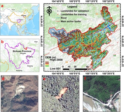
As the first step for LSM, a landslide inventory map was compiled by collecting field observed high accuracy data provided by the local land management department. Till the end of 2019, 304 major slope failures, mainly including small/medium-sized landslides, rock falls and unstable slopes, were recorded and compiled to constitute the core information of landslide inventory (as shown in Figure 1). Since the detailed landslide scarp or boundary was not available in this study, the centroid of the landslide was used to represent the landslide and has been proven its feasibility in LSM (Dou et al. 2020; Huang et al. 2022; Hussin et al. 2016). To avoid training samples imbalance, we randomly sampled the same number of non-landslide points by using the ArcGIS tools. Considering the size of landslides, an empirical value (100-meter) was set to generate the buffer zone of landslide points, and non-landslides were sampled outside this buffer zone. Then, these landslide and non-landslide points were randomly divided into a moderate proportion (7:3) for training and validation purposes.

Subsequently, fifteen conditioning factors were derived from different data sources, as presented in Table 1 and Figure 2, including topographical factors (slope, aspect, elevation, relief amplitude, plan curvature and profile curvature), geological factors (lithology and distance to faults), environmental factors (distance to roads, land-use/cover (LULC), normalized difference vegetation index (NDVI)), hydrological factors (distance to rivers, stream power index (SPI) and topographic wetness index (TWI)) and meteorological factor (annual precipitation).

Figure 2. Fifteen landslide conditioning factors are utilized in LSM.

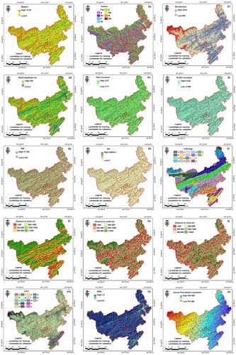
Table 1. Data utilized in the present study.

Source	Format	Time	Scale	Factor
Landslides	Shapefile	2019	–	–
ASTER DEM (https://www.usgs.gov)	TIFF	2011	30 m	Slope
				Aspect
				Elevation
				Relief amplitude
				Plan curvature
				Profile curvature
				TWI
				SPI
Geological map	Shapefile	–	1:500,000	Lithology
				Distance to faults
Road map (http://www.webmap.cn)	Shapefile	2017	1:250,000	Distance to roads
River map (http://www.webmap.cn)	Shapefile	2017	1:250,000	Distance to rivers
LULC map (http://doi.org/10.5281/zenodo.4280923)	TIFF	2020	30 m	LULC
Landsat 8	TIFF	May, 2020	30 m	NDVI
Meteorological observation station data	Shapefile	1989–2019	–	Annual Precipitation

A 30 × 30 m digital elevation model (DEM) was adopted for extracting topographical factors. Among these factors, slope, aspect, elevation factors are the most frequently applied topographical factors in landslide-related studies (Van Den Eeckhaut et al. 2009; Yi et al. 2019), which indicates that they have an important contribution to the occurrence of landslides. In the study area, the terrain slope varies from 0° to 73°. Over 50% of landslides occurred in the region where the slope angle is more than 40° and the elevation is less than 1000 m. In addition, plan curvature and profile curvature can depict the structure and morphology of regional terrain, and relief amplitude measures topographic changes. Thus, these three conditioning factors were also considered in this study.

For geological factors, lithology has a controlling effect on the occurrence of landslides. In the study area, lithology includes 18 groups, and group c and group h are the most widely distributed. A detailed lithology map was presented in Figure 2(i) and Table 2. As the major causative fault in the 2008 Wenchuan earthquake, Yingxiu-Beichuan fault runs through the study area. In addition, there are also Pingwu-Qingchuan and Jiangyou-Guanxian active faults that may promote the occurrence of landslides. Thus, distance to faults was also an essential factor affecting the stability of a slope.

Table 2. Description of the lithology map and LULC map.

Legend number	Lithology	LULC
a	Granite	Rainfed cropland
b	Metavolcanics	Herbaceous cover
c	Slate, limestone and sandstone	Irrigated cropland
d	Schist and tuff	Open evergreen broadleaved forest
e	Diorite	Closed evergreen broadleaved forest
f	Dolomite, limestone and marble	Open deciduous broadleaved forest (0.15 < fc < 0.4)
g	Limestone, shale and siltstone	Closed deciduous broadleaved forest (fc > 0.4)
h		Open evergreen needle-leaved forest (0.15 < fc < 0.4)
i	Slate intercalated with tuff, metasandstone and pebbly sandstone	Closed evergreen needle-leaved forest (fc >0.4)
j	Phyllite, slate, metasandstone, marl and marble	Deciduous shrubland
k	Pyroclastic rock	Grassland
l	Siliceous rock, slate and phyllite	Sparse vegetation (fc < 0.15)
m	Dolomite, sandstone and shale	Wetlands
n	Sandstone and siltstone	Impervious surfaces
o	Shale, limestone and marl	Bare areas
p	Bioclastic limestone	Consolidated bare areas
q	carbonate rock and clastic	Water body
r	Mudstone and siltstone	Permanent ice and snow

For environmental conditions, road excavation usually forms highwall slope and can damage the stability of the slope, promoting landslides. LULC can directly reflect the impact of human activity (e.g. deforestation, agricultural activities) (Meneses, Pereira, and Reis 2019) and poses an impact on the stability of the slope. LULC map was extracted from GLC_FCS30-2020 global land-cover products (Zhang et al. 2021), as presented in Figure 2(m) and Table 2. In addition, vegetation coverage has indirect effects on slope stability by affecting soil erosion (Yi et al. 2019). As a common indicator reflecting vegetation coverage, the NDVI map was calculated by using Landsat-8 imagery, and its value was normalized to [0, 1].

For hydrological factors, SPI and TWI were derived from DEM data. Rivers weaken the slope stability by eroding or saturating slope materials (Yi et al. 2020). SPI measures the erosive capacity of the stream (equation (1)) while TWI reflects the soil moisture spatial pattern (equation (2)) (Sameen, Pradhan, and Lee 2020). Obviously, slope instability is closely related to the hydrological process, e.g. runoff and slope saturation by water (Highland and Bobrowsky 2008). Therefore, distance to rivers, SPI and TWI were considered in this study. (1) $SPI=A_S\times \tan \beta$(1) (2) $TWI=\ln (A_S/\tan \beta )$(2) where A_S is the upslope area per unit contour length and β is the slope gradient in degree.

For the meteorological factor, precipitation is an important trigger factor, which can not only activate old landslides but also trigger new ones. Therefore, the meteorological observation station data, which were recorded from 1989 to 2019, were collected to construct the mean annual precipitation map of the study area.

Finally, to facilitate processing, all landslide conditioning factors were downscaled or interpolated to a resolution of 30 m with the same spatial projection.

3. Methodology

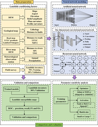
As depicted in Figure 3, this study was mainly conducted in the following three steps. First, various data were collected and processed, including conditioning factors and landslide inventory maps. Then, three neural networks, i.e. ANN, ID CNN and RNN, were constructed to produce the landslide susceptibility maps. Finally, results were compared, evaluated and discussed.

Figure 3. Workflow of the present study.

3.1. Selection of conditioning factors

Before modeling the susceptibility, a crucial step is to check the multicollinearity among these landslide conditioning factors. Because the presence of correlation between conditioning factors may potentially cause incorrect modeling results. In this study, variance inflation factor (VIF) and tolerance (TOL) were adopted to check the multicollinearity. Given the independent variable x, R_j² is the coefficient of determination between the independent variable x_j and the rest of the independent variables. The VIF and TOL can be calculated as follows: (3) $VIF={\displaystyle \frac{1}{(1-R_j^2)}={\displaystyle \frac{1}{TOL}}}$(3) According to some studies (Dou et al. 2020; Yi et al. 2020), the value of VIF is lower than 10 and the value of TOL is greater than 0.1, indicating that these variables are independent of each other.

In addition, the information gain ratio (IGR) method was also applied to analyze the contribution of landslide conditioning factors to modeling. The IGR is a probability-based metric that is primarily applied to evaluate the reduction of uncertainty. Thus, the IGR is usually used for feature selection in many studies (Bui et al. 2020). Generally, the IGR values greater than zero are helpful for landslide modeling, and larger IGR values indicate more useful for modeling.

3.2. Neural network models

3.2.1. ANN

ANN is a commonly used shallow multilayer perceptron method, which can model the complex relationships between conditioning factors and responses. ANN model has several advantages over traditional statistical methods, e.g. high accuracy, self-learning and strong robustness (Yilmaz 2010). Structurally, a typical three-layer ANN includes an input layer, a hidden layer and an output layer (Yi et al. 2020), as illustrated in Figure 4. Each layer has corresponding neurons (one or more), and neurons between different layers are connected by weights. Usually, these weights are continuously adjusted by the back-propagation learning algorithm.

Figure 4. Architecture of a typical three-layer ANN. @15 represents the neurons in this layer are 15.

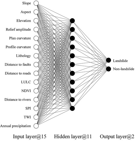
In this study, the input layer refers to the conditioning factors, and the hidden layer mainly acts as the non-linear function to model the complex relationship between landslides and conditioning factors. Theoretically, a simple neural network with one hidden layer is sufficient to simulate most complex functions as long as there are enough neurons in the hidden layer (Hornik 1991). Thus, one hidden layer was used in this study. In addition, to better train the model, the batch normalization layer was added behind the hidden layer. Due to the limited number of neurons, the dropout layer was not applied in the model. Finally, the output layer generates a binary result (i.e. landslide or non-landslide).

3.2.2. 1D CNN

One-dimensional (1D) CNN is a version of a convolutional neural network, which is mainly used to analyze 1D data, such as text data and time-series signal data. Typically, 1D CNN contains the input layer, convolutional layer, pooling layer, fully connected layer and output layer, as presented in Figure 5. Specifically, the convolutional layer is mainly used to extract various data features related to the target and its main role is as a feature extractor. The pooling layer operates on one dimension and is very effective in reducing the amount of data. For a complex task, 1D CNN usually consists of multiple convolutional and pooling layers to learn the complex data features. Finally, the fully connected layer acts as a classifier to classify the extracted data features.

Figure 5. Architecture of 1D CNN.

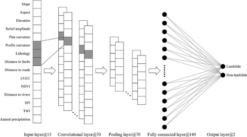
In the present study, to keep the structure simple, a convolutional layer, a pooling layer and a fully-connected layer were adopted to build the 1D CNN model. In addition, the batch normalization layer was added behind the convolutional layer and fully connected layer. To alleviate the over-fitting problems, the dropout layer with a dropout rate of 0.5 was added behind the fully connected layer.

3.2.3. RNN

RNN has been widely used in serialized data processing, such as text language and audio processing. For serialized data, the current data are usually related to the previous data. The implicit relationship is not considered in other neural networks, because the units in the layer are independent and not connected, except RNN. As shown in Figure 6, in the hidden layer of RNN, each unit is connected to other units at different time intervals. In other words, the current output (y_t+1) considers not only the present input (x_t+1), but also the history information of previous elements (such as x_t and x_t-1) of a sequence. Thus, RNN can learn valuable information in sequence data of various lengths (Fang et al. 2020).

Figure 6. Architecture of a typical RNN.

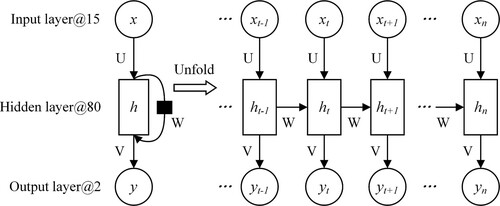
In this study, the landslide conditioning factors were regarded as the one-dimensional serial data, which can be analyzed by the RNN model. The output refers to the landslide or non-landslide. To avoid the over-fitting problems, the alleviate layer with a dropout rate of 0.5 was added behind the hidden layer.

3.3. Accuracy evaluation methods

To quantitatively evaluate the performance of different neural networks, the receiver operating characteristic (ROC) curve was adopted to measure the predictive capabilities of different neural network models (Catani et al. 2013; Dou et al. 2020). Generally, the area under the ROC curve (AUC) varies between 0.5 and 1. An AUC value close to 1 means good performance, and vice versa. In addition, several statistical measures, namely precision, recall, F1 and overall accuracy (OA), were also used to measure the performance of these advanced models (Chen et al. 2018; Yi and Zhang 2020). They can be calculated as follows: (4) $\mathrm{Precision}={\displaystyle \frac{TP}{TP+FP}}$(4) (5) $\mathrm{Recall}={\displaystyle \frac{TP}{TP+FN}}$(5) (6) $F1=2\times {\displaystyle \frac{\mathrm{Precision}\times \mathrm{Recall}}{\mathrm{Precision}+\mathrm{Recall}}}$(6) (7) $OA={\displaystyle \frac{TP+TN}{TP+FP+TN+FN}}$(7) where, TP, FP, TN and FN represent true positive, false positive, true negative and false negative, respectively. For Precision and Recall, the threshold of 0.5 was used to determine the landslide (above 0.5) or non-landslide (below 0.5). Regarding these statistical measures, a higher value indicates the model performs better.

4. Results and discussion

4.1. Multicollinearity and importance analysis

As shown in Figure 7(a), all VIF values were lower than the threshold value (10.0) and all TOL values were greater than 0.1, which implied that there was no significant multicollinearity among the landslide conditioning factors.

Figure 7. (a) Multicollinearity and (b) relative importance analysis of landslide conditioning factors.

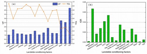
As shown in Figure 7(b), among these factors, topographical factors contributed the most to the susceptibility model, especially the elevation factor. Although these factors (such as SPI, aspect, profile curvature and distance to rivers) contributed little to landslide modeling, their IGR values were higher than zero. Therefore, to make the neural network models better learn the intrinsic features, all selected landslide conditioning factors were adopted to predict the landslide susceptibility.

4.2. Comparison of the performance of neural network models

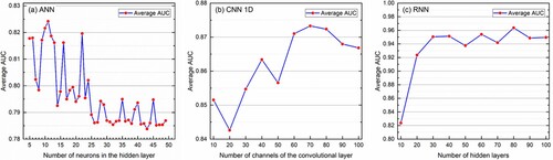
For neural network models, it is very important to choose the appropriate model parameters, including the model structure parameters and the training hyper-parameters. To improve the robustness of neural network models, an effective sampling method, namely the K-fold cross-validation with the stratified sampling, was used in this study. The training data set was internally sampled using tenfold cross-validation. Additionally, to reduce the randomness of training-test split, the stratified sampling strategy was adopted. As shown in Figure 8, the number of neurons in the hidden layers of ANN was set to 11. For 1D CNN, the number of channels of the convolutional layer was set to 70, and the neural units of the fully connected layer were set to 140. Regarding the RNN, the number of hidden layers was set to 80.

Figure 8. Selection of optimal model structure parameters for ANN, 1D CNN and RNN using tenfold cross-validation with the stratified sampling method.

In addition, training hyper-parameter settings are critical to model training; however, there is no universally common standard to select the training hyper-parameters. In this study, training hyper-parameters were determined according to the tenfold cross-validation method, and the details are listed in Table 3. The initial learning rate will dynamically decrease as the number of training epochs increases.

Table 3. Training hyper-parameter setting in this study.

Hyper-parameters	ANN	1D CNN	RNN	Optional parameters
Optimizer	SGD	SGD	SGD	{SGD, Adam, Adagrad, Adadelta}
Activation	ReLU	Tanh	Tanh	{Tanh, ReLU, Sigmoid}
Batch size	120	40	80	{40, 80, 120, 160, 200, 240, 280}
Initial learning rate	0.001	0.001	0.001	{0.001–1 × 10^−9}
Maximum number of epochs	500	500	500	{0–1000}

The landslide susceptibility rate ranges between 0.0 and 1.0, while higher values (close to 1.0) indicate this region is more prone to landslides, and vise-a-versa. To facilitate the analysis, three susceptibility maps derived from ANN, 1D CNN and RNN were reclassified into five landslide susceptibility levels from very high to very low by using the natural breaks method with ArcGIS software, as depicted in Figure 9(a)–(c) respectively.

Figure 9. Landslide susceptibility maps generated by three neural network models.

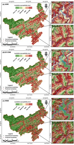
It was observed that the spatial distribution of landslide susceptibility levels obtained by three neural network models was basically consistent, with some slight differences. Visually, the very low susceptibility areas generated by the RNN model were significantly higher than those of ANN and 1D CNN models, which were mostly concentrated in the northwest of the study area. The moderate and high susceptibility areas produced by RNN model were smaller than those of the other two models. For the very high susceptibility level, the areas were mainly distributed in the south and southeast of the study area. For further comparison, two regions (Subarea 1 and subarea 2) were enlarged to display the differences. For subarea 1, the very high and high susceptibility areas were mainly concentrated along the banks of the Pailung River. It is worthwhile to note that the Pailung River was classified as the moderate and low susceptibility areas by ANN and 1D CNN models, while the RNN model divided it into very low susceptibility areas. Obviously, the susceptibility map of this subarea generated by RNN model was more reasonable. In this case, the results generated by ANN and 1D CNN models were relatively more conservative than the RNN model. For subarea 2, the very high and high susceptibility areas generated by the 1D CNN model were larger than those of the other two models, which were mainly distributed along the rivers. Meanwhile, most of the existing landslides were located in these areas. In addition, it can be observed that most landslides in this area were predicted by the three models, which confirmed their good predictive ability.

The mean and standard deviation (Std) of the three susceptibility maps are as follows: RNN (Mean = 0.3366, Std = 0.4082), 1D CNN (Mean = 0.3573, Std = 0.3006) and ANN (Mean = 0.4461, Std = 0.2682). The mean value of the susceptibility map generated by the RNN model is significantly lower than the results of the other two models, while the standard deviation of the RNN model is the highest. It implies that the predicted results of the RNN model are generally low, and the results of the RNN model seem to be more extreme and better than those of ANN and 1D CNN models. In contrast, the predicted results of the ANN model are larger and more conservative, while the results of the 1D CNN model are more balanced. As depicted in Table 4, results revealed that in the resultant maps by ANN, 1D CNN and RNN, very high susceptibility level covered 19.43%, 15.52% and 23.62% of the entire study area, respectively, while very low susceptibility level covered 28.30%, 36.13% and 54.09% of the entire study area, respectively. Obviously, results generated by the RNN model are mainly in the very high and very low susceptibility zones, which is consistent with the statistical results. Furthermore, the percentage of landslides and landslide density values gradually increase with the increase of landslide susceptible levels, demonstrating the feasibility and reliability of the three neural network models.

Table 4. Statistical analysis of different landslide susceptibility maps.

Models	Susceptibility levels	Area (km^2)	Percentage of area	Number of landslides	Percentage of number	Density
ANN	Very low	911.55	28.30%	2	0.66%	0.06
	Low	597.46	18.55%	22	7.24%	1.08
	Moderate	536.94	16.67%	50	16.45%	2.74
	High	549.05	17.05%	66	21.71%	3.54
	Very high	625.92	19.43%	164	53.95%	7.71
1D CNN	Very low	1163.78	36.13%	5	1.64%	0.13
	Low	562.87	17.48%	14	4.61%	0.73
	Moderate	500.81	15.55%	38	12.50%	2.23
	High	493.57	15.32%	67	22.04%	3.99
	Very high	499.87	15.52%	180	59.21%	10.59
RNN	Very low	1742.20	54.09%	12	3.95%	0.20
	Low	290.94	9.03%	13	4.28%	1.31
	Moderate	204.19	6.34%	17	5.59%	2.45
	High	222.82	6.92%	43	14.14%	5.68
	Very high	760.76	23.62%	219	72.04%	8.47

Figure 10 presents the accuracy evaluation results of the three neural network models. Obviously, all the AUC values are higher than 80%, indicating that these neural network models are effective for LSM. Furthermore, the RNN model has the best performance with an AUC of 84.76%, slightly higher than the 1D CNN model with an AUC of 84.59%. ANN model achieved the lowest AUC value (82.90%). For statistical measures (Figure 10(b)), it was observed that most accuracy evaluation measures of the RNN model were higher than those of the other two models. The performance of the 1D CNN model was slightly lower than the RNN model but better than the ANN model. It is worthwhile to note that ANN has the highest recall value, implying ANN was more effective in reducing the occurrence of FN. RNN has the highest precision value, implying the RNN model predicted landslides more accurately. In contrast, the results of the 1D CNN model are more balanced. Additionally, the Wilcoxon rank-sum statistical test (two-tailed) was performed to assess the level of significance between different neural network models. As shown in Table 5, all the P values were less than 0.05, indicating a significant difference between these susceptibility models.

Figure 10. Comparison of the performance of neural network models: (a) ROC curves and (b) histogram of all accuracy evaluation measures.

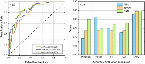
Table 5. Wilcoxon rank-sum statistical test (two-tailed) between different neural network models.

Pairwise	Statistic	P value	Significance
ANN ∼ 1D CNN	502.2134	0.0000	Yes
ANN ∼ RNN	693.4044	0.0000	Yes
1D CNN ∼RNN	463.0361	0.0000	Yes

4.3. Impact of training hyper-parameters and model complexity

For neural network models, the setting of training hyper-parameters not only strongly affects the training process of models but also affects the prediction accuracy. However, different training hyper-parameters have different effects on neural network models, and not all neural network models are affected to the same degree (Wang et al. 2020a). Therefore, investigating the impact of training hyper-parameters on neural network models is very important for the better application of neural network models, as well as the selection of the appropriate LSM model.

Usually, training hyper-parameter of neural network models includes activation function, optimizer, learning rate, batch size and epoch. The activate function is mainly used to introduce nonlinear transformation into neural networks. In order to minimize the training loss, the optimizer is usually adopted to adjust the model weights during the training process, and the learning rate controls the update speed of model weights. The batch size means the number of training data trained in each iteration, and the epoch refers to the number of times to train all training data.

In this study, three main hyper-parameters, i.e. activation function, optimizer and batch size, were analyzed using a trial-and-error approach. For the other two hyper-parameters, we adopted adaptive methods to update them dynamically. For instance, we used an adaptive learning rate to train the three models and applied the early-stopping method to determine the epoch.

As shown in Figure 11, 1D CNN and RNN models achieved the highest AUC values when using the combination of Tanh + SGD, while the ANN model obtained the highest AUC value when using the combination of ReLU + SGD. Specifically, for ANN and 1D CNN models, SGD and Adam optimizers perform better than the other two optimizers (i.e. Adagrad and Adadelta). There is no significant difference in the performance of different activation functions, which implies that ANN and 1D CNN models may not be sensitive to the activation function. For the RNN model, the AUC values of using Tanh and ReLU activation functions are significantly higher than that using the Sigmoid activation function. Also, the performance of RNN model using SGD and Adam optimizers is better than the other two optimizers, which implies that SGD and Adam optimizers are robust in terms of optimizing parameters. In general, the combination of Tanh + SGD was more suitable for this study than other hyper-parameter combinations.

Figure 11. Predictive performance of different neural network models with different training hyper-parameter settings.

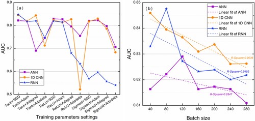
In terms of batch size (Figure 11(b)), it is observed that the highest AUC values were achieved for ANN, 1D CNN and RNN models when batch size was set to 120, 40 and 80, respectively. Specifically, for ANN and RNN models, as the batch size value increases, the AUC values show a trend of increasing and then decreasing, similar to a quadratic function curve. For 1D CNN, as the batch size value increases, the AUC values decrease significantly. Obviously, relatively small batch size values are recommended to improve the performance of neural network models for LSM, especially for the 1D CNN model.

In practice, the selection of a neural network model should not only consider the performance of the model but also consider the complexity. To investigate the complexity of three neural network models used in this study, their model parameters, training and inference time were simply compared in the same windows environment (Intel Core i5-9300H CPU with 8G RAM and NVIDIA GTX 1650 GPU with 4G RAM), as depicted in Table 6.

Table 6. Comparison of model complexity.

Model	Parameters	Training time (ms/epoch)	Inference time (s)
ANN	244	5	7.038
1D CNN	60342	7	17.184
RNN	6722	10	14.058

It can be observed that the ANN model has the least model parameters, followed by RNN and 1D CNN. Meanwhile, compared with the other two models, the ANN model also requires the least training and inference time, implying the relatively low complexity of the ANN model. Although the complexity of 1D CNN and RNN models is relatively high, they performed better than ANN model. Obviously, there is no perfect model. In practice, users should select the appropriate neural network model according to the specific application scenarios.

4.4. Previous studies and future recommendations

In the last few decades, many approaches have been developed for LSM, among which neural network-based methods performed excellently (Thi Ngo et al. 2021; Yi et al. 2020). However, how to select an appropriate neural network model has always been controversial. In addition, although some experiments have proved the effectiveness of neural network models; unfortunately, few studies mentioned their implementation strategies, which makes it difficult for others to adopt these advanced algorithms.

In terms of model structure, there is no widely accepted approach to design the model structure of neural networks. Neural networks are very complex algorithms requires extensive experience in model design, training and fine-tuning. Moreover, differences in topographic conditions may make it difficult to adapt models trained in one region to other regions. Thus, in practice, the K-fold cross-validation method should be applied to determine the structural parameters of neural networks. Additionally, due to a large number of model parameters, dropout layer, adaptive learning rate and early-stopping strategies should be considered during model training.

In terms of training hyper-parameters, we found that relatively small batch size values were effective to improve the performance of neural network models for LSM. Previous studies were also consistent with our findings. For instance, Wang et al. (2020a) reported 32 and 64 are the optimal batch size, compared to 128 and 256. Sameen, Pradhan, and Lee (2020) reported the optimal batch size is 16 for CNN when batch size varies between 4 and 128. Hua et al. (2021) stated the optimal batch size is 600 for DNN when batch size varies between 20 and 3000. It is worth noting that the value of batch size may be related to the number of training samples. Because the number of training samples in most LSM studies is relatively small compared to other image-related tasks. This conjecture needs to be further confirmed. In terms of activation function and optimizer, ReLU activation function and Adam optimizer were commonly used in many studies (Lv et al. 2022; Wang et al. 2020a). However, based on extensive experiments, we found that the Tanh activation function performs more robustly than the ReLU activation function, and SGD optimizer also performs slightly better than Adam optimizer. It may be related to the properties of the training sample and requires further investigation in the future.

In addition, neural network models require a large number of reliable training samples as input, which implies that the sampling strategy and ratio of landslide/non-landslide samples should be taken into account seriously. For this study, we adopted the buffer-based non-landslide sampling method that is commonly used method in LSM. However, unreasonable buffer distance settings may lead to biased non-landslide samples (Lucchese, de Oliveira, and Pedrollo 2021). The impact of sampling strategy on neural network models needs to be further analyzed in the future. It should also be noted that the study area and training samples in this study were relatively small, and the division ratio between train and validation samples (7:3) is moderate and acceptable. For continental or global susceptibility mapping, the division ratio, as well as the model structure and optimal hyper-parameter values for neural network models, may need to be adjusted according to the amount of data.

5. Conclusions

In this study, three neural network models, i.e. ANN, 1D CNN and RNN, were investigated and evaluated in terms of their performances for LSM in the Qingchuan County, Sichuan province, China. Through comprehensive experiments, the following remarks can be concluded:

• ●Three neural network models can accurately identify landslide susceptible regions. Spatially, the zonation of landslide susceptibility levels generated by ANN and 1D CNN models was basically consistent, but slightly differed from that of the RNN model. Qualitative and quantitative evaluation results, however, suggested that the RNN model performed better among the three neural network models.

• ●The Tanh activation function and SGD optimizer were found more suitable for training neural network models in this study, and relatively small batch size values were recommended to improve the performance of neural network models for LSM, especially for the 1D CNN model.

• ●ANN model requires the least model parameters, training and inference time, implying it owns relative low complexity, followed by 1D CNN and RNN models. However, the RNN model achieved the highest accuracy values among the three neural network models. It indicated that no perfect model exists for LSM, and the selection of the neural network model in LSM should be based on the specific application scenarios.

In general, this study provided insights and scientific suggestions for LSM using neural network models, which is expected to help those who apply these advanced methods to improve their efficiency. Furthermore, an easy-to-use software based on neural networks should be developed in the future to enhance landslide understanding and monitoring capabilities. Additionally, it is recommended to explore the impact of more parameters on neural network models and evaluate these models in many extensive regions.

Disclosure statement

No potential conflict of interest was reported by the author(s).

Data availability statement

The data or code used in this study are available from the corresponding author on reasonable request.

Additional information

Funding

This work was supported by the National Natural Science Foundation of China [grant number 41941016, U1839204 and U2139201]; National Institute of Natural Hazards, Ministry of Emergency Management of China Research Fund [grant number ZDJ2017-24].

References

- Abbaszadeh Shahri, Abbas, Johan Spross, Fredrik Johansson, and Stefan Larsson. 2019. “Landslide Susceptibility Hazard Map in Southwest Sweden Using Artificial Neural Network.” Catena 183: 104225.
- Ali, Sk Ajim, Farhana Parvin, Jana Vojteková, Romulus Costache, Nguyen Thi Thuy Linh, Quoc Bao Pham, Matej Vojtek, Ljubomir Gigović, Ateeque Ahmad, and Mohammad Ali Ghorbani. 2021. “GIS-based Landslide Susceptibility Modeling: A Comparison Between Fuzzy Multi-Criteria and Machine Learning Algorithms.” Geoscience Frontiers 12 (2): 857–876.
- Bui, Dieu Tien, Paraskevas Tsangaratos, Viet-Tien Nguyen, Ngo Van Liem, and Phan Trong Trinh. 2020. “Comparing the Prediction Performance of a Deep Learning Neural Network Model with Conventional Machine Learning Models in Landslide Susceptibility Assessment.” Catena 188: 104426.
- Catani, F., D. Lagomarsino, S. Segoni, and V. Tofani. 2013. “Landslide Susceptibility Estimation by Random Forests Technique: Sensitivity and Scaling Issues.” Natural Hazards and Earth System Sciences 13 (11): 2815–2831.
- Chen, Wei, Shuai Zhang, Renwei Li, and Himan Shahabi. 2018. “Performance Evaluation of the GIS-Based Data Mining Techniques of Best-First Decision Tree, Random Forest, and Naïve Bayes Tree for Landslide Susceptibility Modeling.” Science of The Total Environment 644: 1006–1018.
- Cruden, David, and D. J. Varnes. 1996. “Landslide Types and Processes.” In Landslides: Investigation and Mitigation, edited by A. K. Turner and R. L. Schuster, 36–75. Washington, D.C: National Academy Press. Vol. 247.
- Dai, F. C., and C. F. Lee. 2002. “Landslide Characteristics and, Slope Instability Modeling Using GIS, Lantau Island, Hong Kong.” Geomorphology 42 (3–4): 213–228.
- Dao, Dong Van, Abolfazl Jaafari, Mahmoud Bayat, Davood Mafi-Gholami, Chongchong Qi, Hossein Moayedi, Tran Van Phong, et al. 2020. “A Spatially Explicit Deep Learning Neural Network Model for the Prediction of Landslide Susceptibility.” Catena 188: 104451.
- Dou, Jie, Hiromitsu Yamagishi, Hamid Reza Pourghasemi, Ali P. Yunus, Xuan Song, Yueren Xu, and Zhongfan Zhu. 2015. “An Integrated Artificial Neural Network Model for the Landslide Susceptibility Assessment of Osado Island, Japan.” Natural Hazards 78 (3): 1749–1776.
- Dou, Jie, Ali P. Yunus, Abdelaziz Merghadi, Ataollah Shirzadi, Hoang Nguyen, Yawar Hussain, Ram Avtar, Yulong Chen, Binh Thai Pham, and Hiromitsu Yamagishi. 2020. “Different Sampling Strategies for Predicting Landslide Susceptibilities are Deemed Less Consequential with Deep Learning.” Science of The Total Environment 720: 137320.
- Fan, Xuanmei, Ali P. Yunus, Gianvito Scaringi, Filippo Catani, Srikrishnan Siva Subramanian, Qiang Xu, and Runqui Huang. 2021. “Rapidly Evolving Controls of Landslides After a Strong Earthquake and Implications for Hazard Assessments.” Geophysical Research Letters 48 (1): e2020GL090509.
- Fang, Zhice, Yi Wang, Ling Peng, and Haoyuan Hong. 2020. “A Comparative Study of Heterogeneous Ensemble-Learning Techniques for Landslide Susceptibility Mapping.” International Journal of Geographical Information Science 35 (2): 321–347.
- Fell, Robin, Jordi Corominas, Christophe Bonnard, Leonardo Cascini, Eric Leroi, and William Z. Savage. 2008. “Guidelines for Landslide Susceptibility, Hazard and Risk Zoning for Land Use Planning.” Engineering Geology 102 (3–4): 85–98.
- Froude, M. J., and D. N. Petley. 2018. “Global Fatal Landslide Occurrence from 2004 to 2016.” Natural Hazards and Earth System Sciences 18 (8): 2161–2181.
- Gariano, Stefano Luigi, and Fausto Guzzetti. 2016. “Landslides in a Changing Climate.” Earth-Science Reviews 162: 227–252.
- Goetz, J. N., A. Brenning, H. Petschko, and P. Leopold. 2015. “Evaluating Machine Learning and Statistical Prediction Techniques for Landslide Susceptibility Modeling.” Computers & Geosciences 81: 1–11.
- Gorsevski, Pece V., M. Kenneth Brown, Kurt Panter, Charles M. Onasch, Anita Simic, and Jeffrey Snyder. 2016. “Landslide Detection and Susceptibility Mapping Using LiDAR and an Artificial Neural Network Approach: A Case Study in the Cuyahoga Valley National Park, Ohio.” Landslides 13 (3): 467–484.
- Guzzetti, F., P. Reichenbach, M. Cardinali, M. Galli, and F. Ardizzone. 2005. “Probabilistic Landslide Hazard Assessment at the Basin Scale.” Geomorphology 72 (1–4): 272–299.
- Habumugisha, Jules Maurice, Ningsheng Chen, Mahfuzur Rahman, Md Monirul Islam, Hilal Ahmad, Ahmed Elbeltagi, Gitika Sharma, Sharmina Naznin Liza, and Ashraf Dewan. 2022. “Landslide Susceptibility Mapping with Deep Learning Algorithms.” Sustainability 14: 3.
- He, Qian, Ming Wang, and Kai Liu. 2021. “Rapidly Assessing Earthquake-Induced Landslide Susceptibility on a Global Scale Using Random Forest.” Geomorphology 391: 107889.
- Highland, Lynn M., and Peter Bobrowsky. 2008. “The Landslide Handbook - A Guide to Understanding Landslides.” Circular 147: 30–33.
- Hong, Haoyuan, Junzhi Liu, Dieu Tien Bui, Biswajeet Pradhan, Tri Dev Acharya, Binh Thai Pham, A. Xing Zhu, Wei Chen, and Baharin Bin Ahmad. 2018. “Landslide Susceptibility Mapping Using J48 Decision Tree with AdaBoost, Bagging and Rotation Forest Ensembles in the Guangchang Area (China).” Catena 163: 399–413.
- Hornik, Kurt. 1991. “Approximation Capabilities of Multilayer Feedforward Networks.” Neural Networks 4 (2): 251–257.
- Hua, Y., X. M. Wang, Y. W. Li, P. Y. Xu, and W. X. Xia. 2021. “Dynamic Development of Landslide Susceptibility Based on Slope Unit and Deep Neural Networks.” Landslides 18 (1): 281–302.
- Huang, Faming, Jun Yan, Xuanmei Fan, Chi Yao, Jinsong Huang, Wei Chen, and Haoyuan Hong. 2022. “Uncertainty Pattern in Landslide Susceptibility Prediction Modelling: Effects of Different Landslide Boundaries and Spatial Shape Expressions.” Geoscience Frontiers 13: 2.
- Hungr, Oldrich, Serge Leroueil, and Luciano Picarelli. 2014. “The Varnes Classification of Landslide Types, an Update.” Landslides 11 (2): 167–194.
- Hussin, Haydar Y., Veronica Zumpano, Paola Reichenbach, Simone Sterlacchini, Mihai Micu, Cees van Westen, and Dan Bălteanu. 2016. “Different Landslide Sampling Strategies in a Grid-Based bi-Variate Statistical Susceptibility Model.” Geomorphology 253: 508–523.
- Jena, Ratiranjan, Biswajeet Pradhan, Nizamuddin Ghassan Beydoun, Hizir Sofyan Ardiansyah, and Muzailin Affan. 2019. “Integrated Model for Earthquake Risk Assessment Using Neural Network and Analytic Hierarchy Process: Aceh Province, Indonesia.” Geoscience Frontiers 11 (2): 613–634.
- LeCun, Yann, Yoshua Bengio, and Geoffrey Hinton. 2015. “Deep Learning.” Nature 521: 436.
- Li, Y., G. Chen, C. Tang, G. Zhou, and L. Zheng. 2012. “Rainfall and Earthquake-Induced Landslide Susceptibility Assessment Using GIS and Artificial Neural Network.” Natural Hazards and Earth System Sciences 12 (8): 2719–2729.
- Lucchese, Luísa Vieira, Guilherme Garcia de Oliveira, and Olavo Correa Pedrollo. 2021. “Investigation of the Influence of Nonoccurrence Sampling on Landslide Susceptibility Assessment Using Artificial Neural Networks.” Catena 198: 105067.
- Lv, Liang, Tao Chen, Jie Dou, and Antonio Plaza. 2022. “A Hybrid Ensemble-Based Deep-Learning Framework for Landslide Susceptibility Mapping.” International Journal of Applied Earth Observation and Geoinformation 108: 102713.
- Mansouri Daneshvar, Mohammad Reza. 2014. “Landslide Susceptibility Zonation Using Analytical Hierarchy Process and GIS for the Bojnurd Region, Northeast of Iran.” Landslides 11 (6): 1079–1091.
- Meneses, Bruno M., Susana Pereira, and Eusébio Reis. 2019. “Effects of Different Land Use and Land Cover Data on the Landslide Susceptibility Zonation of Road Networks.” Natural Hazards and Earth System Sciences 19 (3): 471–487.
- Nsengiyumva, Jean Baptiste, Geping Luo, Amobichukwu Chukwudi Amanambu, Richard Mind'je, Gabriel Habiyaremye, Fidele Karamage, Friday Uchenna Ochege, and Christophe Mupenzi. 2019. “Comparing Probabilistic and Statistical Methods in Landslide Susceptibility Modeling in Rwanda/Centre-Eastern Africa.” Science of The Total Environment 659: 1457–1472.
- Pham, Binh Thai, Abolfazl Jaafari, Trung Nguyen-Thoi, Tran Van Phong, Huu Duy Nguyen, Neelima Satyam, Md Masroor, et al. 2020. “Ensemble Machine Learning Models Based on Reduced Error Pruning Tree for Prediction of Rainfall-Induced Landslides.” International Journal of Digital Earth 14 (5): 575–596.
- Reichenbach, P., M. Rossi, B. D. Malamud, M. Mihir, and F. Guzzetti. 2018. “A Review of Statistically-Based Landslide Susceptibility Models.” Earth-Science Reviews 180: 60–91.
- Sameen, Maher Ibrahim, Biswajeet Pradhan, and Saro Lee. 2020. “Application of Convolutional Neural Networks Featuring Bayesian Optimization for Landslide Susceptibility Assessment.” Catena 186: 104249.
- Thi Ngo, Phuong Thao, Mahdi Panahi, Khabat Khosravi, Omid Ghorbanzadeh, Narges Kariminejad, Artemi Cerda, and Saro Lee. 2021. “Evaluation of Deep Learning Algorithms for National Scale Landslide Susceptibility Mapping of Iran.” Geoscience Frontiers 12 (2): 505–519.
- Van Den Eeckhaut, M., P. Reichenbach, F. Guzzetti, M. Rossi, and J. Poesen. 2009. “Combined Landslide Inventory and Susceptibility Assessment Based on Different Mapping Units: An Example from the Flemish Ardennes, Belgium.” Natural Hazards and Earth System Sciences 9 (2): 507–521.
- Varnes, D. J. 1978. “Slope Movement Types and Processes.” In Landslides: Analysis and Control, edited by R. L. Schuster and R. J. Krizek, 11–33. Washington, DC: Unesco.
- Wang, Yi, Zhice Fang, and Haoyuan Hong. 2019. “Comparison of Convolutional Neural Networks for Landslide Susceptibility Mapping in Yanshan County, China.” Science of The Total Environment 666: 975–993.
- Wang, Yi, Zhice Fang, Mao Wang, Ling Peng, and Haoyuan Hong. 2020a. “Comparative Study of Landslide Susceptibility Mapping with Different Recurrent Neural Networks.” Computers & Geosciences 138: 104445.
- Wang, W. D., Z. L. He, Z. Han, Y. G. Li, J. Dou, and J. L. Huang. 2020b. “Mapping the Susceptibility to Landslides Based on the Deep Belief Network: A Case Study in Sichuan Province, China.” Natural Hazards 103 (3): 3239–3261.
- Wei, Ruilong, Chengming Ye, Tianbo Sui, Yonggang Ge, Yao Li, and Jonathan Li. 2022. “Combining Spatial Response Features and Machine Learning Classifiers for Landslide Susceptibility Mapping.” International Journal of Applied Earth Observation and Geoinformation 107: 102681.
- Wu, Xuan, Zhijie Zhang, Wanchang Zhang, Yaning Yi, Chuanrong Zhang, and Qiang Xu. 2021. “A Convolutional Neural Network Based on Grouping Structure for Scene Classification.” Remote Sensing 13: 13.
- Xu, C., F. C. Dai, X. W. Xu, and Y. H. Lee. 2012. “GIS-based Support Vector Machine Modeling of Earthquake-Triggered Landslide Susceptibility in the Jianjiang River Watershed, China.” Geomorphology 145: 70–80.
- Yi, Yaning, and Wanchang Zhang. 2020. “A New Deep-Learning-Based Approach for Earthquake-Triggered Landslide Detection from Single-Temporal RapidEye Satellite Imagery.” IEEE Journal of Selected Topics in Applied Earth Observations and Remote Sensing 13: 6166–6176.
- Yi, Yaning, Zhijie Zhang, Wanchang Zhang, Huihui Jia, and Jianqiang Zhang. 2020. “Landslide Susceptibility Mapping Using Multiscale Sampling Strategy and Convolutional Neural Network: A Case Study in Jiuzhaigou Region.” Catena 195: 104851.
- Yi, Yaning, Zhijie Zhang, Wanchang Zhang, Qi Xu, Cai Deng, and Qilun Li. 2019. “GIS-based Earthquake-Triggered-Landslide Susceptibility Mapping with an Integrated Weighted Index Model in Jiuzhaigou Region of Sichuan Province, China.” Natural Hazards and Earth System Sciences 19 (9): 1973–1988.
- Yilmaz, Işık. 2010. “The Effect of the Sampling Strategies on the Landslide Susceptibility Mapping by Conditional Probability and Artificial Neural Networks.” Environmental Earth Sciences 60 (3): 505–519.
- Zhang, Xiao, Liangyun Liu, Xidong Chen, Yuan Gao, Shuai Xie, and Jun Mi. 2021. “GLC_FCS30: Global Land-Cover Product with Fine Classification System at 30 m Using Time-Series Landsat Imagery.” Earth System Science Data 13 (6): 2753–2776.
- Zhu, A. X., R. X. Wang, J. P. Qiao, C. Z. Qin, Y. B. Chen, J. Liu, F. Du, Y. Lin, and T. X. Zhu. 2014. “An Expert Knowledge-Based Approach to Landslide Susceptibility Mapping Using GIS and Fuzzy Logic.” Geomorphology 214 (214): 128–138.