Automatic selection of permanent scatterers-based GCPs for refinement and reflattening in InSAR DEM generation

ABSTRACT

In DEM generation using interferometric synthetic aperture radar (InSAR), the ground control points (GCPs) for refinement and reflattening are usually selected by manual selection, field surveying, GPS points and existing basemaps, which may not be completely suitable for consequent processes. We proposed a new method (auto-PS-GCP) of GCP selection based on permanent scatterers, which automatically defines the thresholds for the coherence, amplitude, and amplitude dispersion index to select permanent scatterer as the GCPs. The GCP thinning (auto-PS-GCP-Thin) was further conducted considering the point density, distances among points and terrain conditions. We used a three-stage assessment that includes: (1) phase stability and intensity of the GCPs, (2) RMSEs of the elevations between GCPs and homonymous points in the reference DEM, and (3) generated DEM accuracy. Three areas respectively in the plain, hilly and mountainous regions were selected to verify the proposed methods. The assessment using both SRTM DEM andICESat-2 points shows that the DEM accuracy of auto-PS-GCP-Thin was improved by 20%∼30% for different areas compared to the manual, where the best DEM accuracy of 4.71 m was found in the plain area. It is concluded that the proposed methods are effective and reliable in various areas with different terrain conditions.

KEYWORDS:

• InSAR
• permanent scatterers
• automatic threshold definition
• ground control points
• DEM generation

1. Introduction

Interferometric synthetic aperture radar (InSAR) is a high-precision technique to extract ground elevation and deformation information by deriving phase information from single look complex (SLC) images (Wang et al. 2019). Many institutes are dedicated to the method development of digital elevation model (DEM) generation and the production of DEMs (e.g. SRTM DEM, ASTER G-DEM, and TanDEM-X DEM) at global and local scales, especially using SAR images (Bhardwaj, Jain, and Chatterjee 2019). When using the InSAR techniques, the phase measurement and conversion of phase to height are the essences of the DEM generation. Since SAR typically operates in the microwave region, it can be used in any meteorological conditions and with a full day-and-night operational capability (Zhang et al. 2016; Mohammadi et al. 2020). As a consequence of SAR's flexibility, the InSAR technique is scientific and practical to derive DEMs (Yadav et al. 2020). Although InSAR has the advantages of large region and continuous space coverage, the process of InSAR DEM generation is extremely susceptible to various factors, such as the selection of the interference pair, the baseline, and the atmospheric environments (Pepe and Calò 2017). The introduction of high-quality ground control points (GCPs) in the orbit refinement and reflattening process can correct the baseline parameters and remove the flattening effect to improve the DEM accuracy effectively (Du et al. 2021). However, commonly used selection methods of GCPs such as manual selection could reduce the DEM accuracy (Child et al. 2021). It is necessary to develop new methods to select appropriate GCPs for refinement and reflattening to produce more accurate DEMs.

For refinement and reflattening, useful GCPs can be selected by several methods including manual selection, existing surveying data, artificial corner reflectors, and permanent scatterers (PSs). Among these, the manual selection is a conventional and commonly used method that extracts GCPs for refinement and reflattening in both the subsidence monitoring and the DEM generation (Müller et al. 2012). However, such GCPs are usually extracted by modelers from SAR images (Li et al. 2017), and this is difficult to perform because it is not easy to identify homonymy points from SAR images. As such, the quality of manually selected GCPs is highly related to the modelers’ understudying of SAR images, familiarity with the study area, and experience in SAR processing. In addition, manual selection is time-consuming especially when processing a large number of SAR images (Chureesampant and Susaki 2014).

Existing surveying data can also be used to extract high-quality GCPs to improve the baseline parameters for orbit refinement and remove the interference phase errors, then generate highly accurate InSAR DEMs (Du, Yang, and Shi 2010). Although this is a reliable method, the surveying data may not available for every SAR image and it is time-consuming, laborious and costly when performing field surveying for every study site. In-suit artificial corner reflectors can provide the highest quality GCPs for SAR geometry calibration, radiometric calibration, and InSAR processing (Jauvin, Yan, and Trouvé 2017). However, artificial corner reflectors need professional design and production for different satellites, and should be equipped in the field with accurate coordinates and attitudes (Pan and Liu 2010). This shows that it is time-consuming and costly to design, prepare and equip the artificial corner reflectors on site.

GCPs can also be extracted from PSs that refer to various ground targets with strong scattering, high coherence, and stable phase (Ferretti, Prati, and Rocca 2001). In SAR images, typical PSs usually include the top corners of structures, bridges, railings, and exposed rocks, which are usually presented in a single-pixel or multiple pixels in SAR images according to their resolutions. Because PSs reflect stable facilities and spatial entities, the method is feasible to produce sufficient GCPs for refinement and reflattening to reduce the interferometric phase errors then improve the DEM accuracy. In the literature, the identification and extraction of PSs usually integrate the coherence, averaged-amplitude across images, and the amplitude dispersion index (ADI) across pixels (Dinh, Ramon, and Fabio 2020). Some modelers defined a threshold for the coherence to extract PSs (Berardino et al. 2002), while others used a suitable ADI as threshold (Qu, Wang, and Wen 2011). For example, Zeng et al. (2015) used phase as the criterion to extract PSs for producing DEMs using space borne radar data. In fact, a single criterion such as coherenceor averaged-amplitude only considers one aspect of PSs. Specifically, Mu’amalah, Anjasmara, and Taufik (2021) denoted that the phase dispersion index threshold considers the phase stability and the extracted PSs consequently may likely be sensitive to the decor relation and system noise, and Tian et al. (2019) indicated that the coherence also considers the high signal-to-noise ratio (SNR). Other colleagues (Shirani and Pasandi 2019) showed that the ADI principally considers phase stability, which includes some PSs that may not perform well in refinement and reflattening.

Earlier studies have also made progress in PS-based GCP selection methods (Tian et al. 2019; Xiang et al. 2019). The PS selection needs to consider both the phase stability and the scattering intensity, where appropriate thresholds should be pre-defined to extract suitable points and drop unreliable points. In fact, the interferogram generation is related to the topographic influence (Sosnovsky, Kobernichenko, and Vinogradova 2019), and useful GCPs are usually distributed in flat areas. The terrain slope calculated from elevation should be a suitable metric to help select high-quality GCPs. The distribution and density of the selected GCPs also substantially affect the refinement and reflattening in InSAR (Chen, Peng, and Yang 2017), and calibrating the GCPs by dropping some of them may improve the performance. Therefore, the GCP selection should consider the impacts of terrain conditions and the distribution of GCPs sufficiently. Here, we refer to the intermediate results obtained in the PS selection process as permanent scatterer candidate (PSC), and the final selection result is permanent scatterer. In addition, there are several stages related to GCP selection in InSAR DEM generation, where each stage should be adequately assessed to ensure their validations. Thus, this study aims to address key issues of GCP selection as: (1) can we jointly consider terrain conditions and point density to select suitable GCPs for refinement and reflattening? (2) how to assess the quality and suitability of GCPs at each stage in InSAR DEM generation? and (3) how well do the GCP selection methods perform in areas of different terrain types?

To address the above questions, we developed a new method (auto-PS-GCP-Thin) that considers the phase, scattering, coherence, terrain slope, and point distribution to extract more reliable and useful GCPs, hence producing more accurate DEMs using InSAR. The method was applied to InSAR DEM generation in a plain area, a hilly area, and a mountainous area. To prove the effectiveness of this method, we chose Sentinel-1A with small orbital tubes as the experimental data. The Sentinel-1A's baselines are usually small thus it is difficult to derive a good height resolution. If the proposedmethod has obvious improvement in the DEM generation using Sentinel-1A, it will produce much better DEM products when using better SAR images such as TerraSAR images. In this study, an integrated three-stage assessment approach was then applied to evaluate the GCP selection method, the GCPs themselves, and the generated DEMs. The methods shouldbe useful to automatically extract high-quality GCPs elsewhere when producing accurate DEMs using InSAR.

2. Methodology

2.1. The InSAR DEM generation method

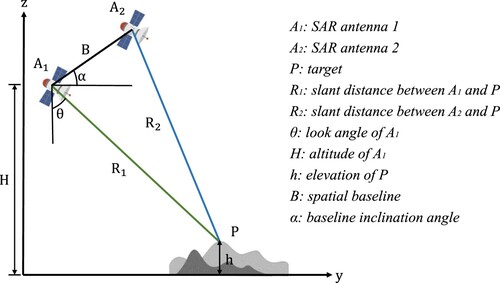
DEM generation by InSAR needs height measurement using repeated observation data (SAR images) of the same area through simultaneous observation by two pairs of antennas or by two parallel observations (Wegmuller et al. 2008). A pair of SAR images exist phase differences, which can be combined with the orbit parameters of the observation platform to generate high-precision and high-resolution ground elevation information (Zhao 2016). As shown in Figure 1, the recorded phases (φ₁ and φ₂) of the same target (P) are different due to the difference in the distances between the satellite and the target during the two observations. The interference phase (φ_int) is given by: (1) ${\phi }_{int}={\phi }_1-{\phi }_2=-{\displaystyle \frac{2\pi }{\lambda }\left(R_1-R_2\right)=-{\displaystyle \frac{2\pi }{\lambda }\mathrm{\Delta }R}}$(1) where φ₁ and φ₂ are the phases of the echo signal from the target, λ is the radar wavelength, R₁ and R₂ are the distances from the two antennas to the observation target P, and ΔR isthe difference in the distances.

Figure 1. The geometric relationships between the target and the SAR spaceborne.

The interference phase (φ_int) consists of the terrain phase (φ_top), terrain deformation phase (φ_def), flattening effect phase (φ_flat), atmospheric phase (φ_atm), and noise phase (φ_noi): (2) ${\phi }_{int}={\phi }_{top}+{\phi }_{def}+{\phi }_{flat}+{\phi }_{atm}+{\phi }_{noi}$(2) where the true terrain phase (φ_top) of the target is obtained after removing the flattening effect, atmospheric, and noise phases. Thus, based on the geometric relationship shown in Figure 1, the elevation (h) of the target (P) can be given by (Rosen et al. 2000): (3) $h=H-{\displaystyle \frac{\left({\displaystyle \frac{\lambda {\phi }_{top}}{4\pi }}\right)-B^2}{2Bsin\left(\theta -\alpha \right)-{\displaystyle \frac{\lambda {\phi }_{top}}{2\pi }}}cos\theta }$(3) where B is the spatial baseline between SAR antennas A₁ and A₂, H and θ are the altitude and the look angle of A₁, and α isthe baseline inclination angle.

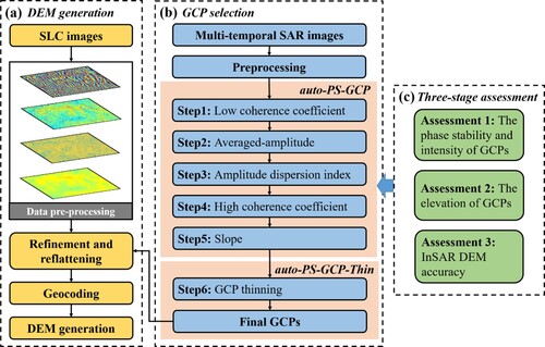
Stable and high-quality GCPs can effectively improve the performance of orbit refinement and reflattening, thereby improving the generated DEM accuracy. We then proposed an auto-PS-GCP selection method for orbit refinement and reflattening. Figure 2 shows the workflow that consists of three steps: (a) the InSAR DEM generation; (b) the auto-PS-GCP and the auto-PS-GCP-thin selection; (c) the three-stage assessment. We finally applied the auto-PS-GCP and auto-PS-GCP-Thin methods to multi-temporal SAR images in three sites (each in plains, hilly areas, and mountainous areas) to verify the methods. The selected GCPs were transformed into the slant-range coordinate system and applied to the InSAR processing. According to the three-stage assessment, we evaluated the phase stability and scattering intensity of the selected GCPs, their elevation accuracies, and the generated InSAR DEMs.

Figure 2. The workflow of auto-PS-GCP for refinement and reflattening in InSAR DEM generation.

2.2. The auto-PS-GCP selection method

The auto-PS-GCP selection method considers temporal stability and spatial continuity to select a suitable number of PSs. Based on PS selection, the GCPs are selected successively by automatic evaluation of coherence, averaged-amplitude and ADI, and the GCP thinning as shown in Figure 2, which have been addressed as follows. To ensure that the amplitude of all images can truly reflect the scattering of the ground targets, we carried out radiometric calibration before selecting GCPs.

2.2.1. The coherence coefficient

The coherence (γ) is the first criterion to extract PSs. It is estimated by the complex number of adjacent pixels in a square window (e.g. 3×3). The calculation method is given by (Marotti et al. 2008): (4) $\gamma ={\displaystyle \frac{\left|{\sum }_{i=1}^a{\sum }_{j=1}^{b}M\left(i,j\right)S^{\ast }\left(i,j\right)\right|}{\sqrt{{\sum }_{i=1}^a{\sum }_{j=1}^b{\left|M\left(i,j\right)\right|}^2{\sum }_{i=1}^a{\sum }_{j=1}^b{\left|S\left(i,j\right)\right|}^2}}}$(4) where M(i,j) is the complex number of the master SAR image, S(i,j) is the complex number of the slave SAR image, and these two images constitute the interference pair, i is the row and j is the column in the square window, the asterisk is the conjugate operator of complex numbers, and a and b represent the window sizes (here a = b = 3). The SNR of a pixel is estimated from its coherence: (5) $SNR={\displaystyle \frac{\gamma }{1+\gamma }}$(5) where a higher coefficient indicates a higher SNR and better quality of the interferogram. Each pixel has an averaged coherence (γ_pix) considering the coherence (γ) of the same pixel in all K-time-series images: (6) $\{\begin{array}{c}{\gamma }_{pix}={\displaystyle \frac{1}{K}\sum _{k=1}^K\gamma }\\ s.t.{\gamma }_{pix}>{\gamma }_{pix-thd}\end{array}$(6) where K indicates the number of SAR images at different times, and k is the k-th image. Thus, the PSC₁ are those with higher coherences compared with a pre-defined threshold (γ_pix-thd). The correlation coefficient is estimated based on the local window (see Equation (4)), which greatly reduces the calculation load of subsequent selection. However, this makes it more difficult to identify useful points (PSC) that are surrounded by ineffective points. Also, thePSC selected by the correlation coefficient need to be filtered using other pixel-level methods.

A small threshold can only remove points with serious decoherence, while a high threshold could miss useful PSC (Xiang et al. 2019). We used a low-threshold of coherence (γ_pix-thd1) to remove areas such as water and vegetation-covered areas (Step 1 in Figure 2).

2.2.2. The averaged-amplitude

Each SAR image has its averaged-amplitude that indicates the scattering intensity, and for all time-series SAR images, there is a minimum (A_img-thd) among these averaged-amplitudes. The minimum averaged-amplitude (Step 2 in Figure 2) is defined as the threshold to extract PSs from SAR images (Liu, Zhang, and Zhao 2020). When comparing to the threshold, we keep a pixel with higher amplitude and if it is found in all SAR images: (7) $\{\begin{array}{c}{A}_{img-thd}=\mathrm{m}\mathrm{i}\mathrm{n}\left\{{\displaystyle \frac{1}{m\times n}\sum _{e=1}^m\sum _{f=1}^n{A}_{k\left(e,f\right)}\left|k=1,\dots ,K\right|}\right\}\\ s.t.A_{img}>A_{img-thd}\end{array}$(7) where (m, n) represents the total row and column of the SAR images that cover the same area, and A_k(e,f) is the amplitude of the pixel at row e and column f in the k-th SAR image. The minimum averaged-amplitude (A_img-thd) is considered the threshold to eliminate the points that have low amplitude but show falsely high coherence in Step 1 to extract PSC₂.

2.2.3. The amplitude dispersion index

The ADI is used as the third criterion (Step 3 in Figure 2) to select PSC₃ (Crosetto et al. 2015). The index can also be used to reflect the phase stability as represented by the phase standard deviation (Ferretti, Prati, and Rocca 2001). Each pixel has an amplitude and K time-series images have K amplitude values for the same pixel. The ADI (A_pix-disp) can be given by: (8) $\{\begin{array}{c}{A}_{pix-disp}={\displaystyle \frac{A_{pix-\sigma }}{A_{pix}}\approx {\sigma }_v}\\ s.t.A_{pix-disp}<A_{pix-disp-thd}\end{array}$(8) where A_pix-σ is the standard deviation of amplitudes and A_pix is the averaged-amplitude for each pixel of the same location across all images. An appropriate threshold (A_pix-disp-thd) is defined to extract the PSs with ADI smaller than the threshold.

This method is not affected by adjacent pixels because it is calculated by the pixels of different images at the same location. The points with serious decoherence are removed from PSCs because we consider the phase stability of each pixel over time. This method in Equation (8) works when applied to pixels with a high SNR, where these pixels are extracted in advance according to Equation (4). Wethen used a high-threshold of coherence (γ_pix-thd2) to further select PSC₄ (Step 4 in Figure 2) to get more credible points.

2.2.4. The terrain slope

We use terrain slope as one of the criteria (Step 5 in Figure 2) for PS selection to reduce the side effects on interference accuracy caused by steep terrain (Li, Liu, and Ding 2006). Steps 1–4 generate PSC₄ with good phase stability and strong scattering intensity, and this step further extracts points in flat areas. Thus, an appropriate threshold (SLOPE_thd) is defined to extract the final PSs from PSC₄ with a slope smaller than SLOPE_thd. The slope can be calculated by: (9) $\{\begin{array}{c}SLOPE=\mathrm{a}\mathrm{r}\mathrm{c}\mathrm{t}\mathrm{a}\mathrm{n}\sqrt{p^2+q^2}\times {\displaystyle \frac{180}{\pi }}\\ s.t.SLOPE<SLOP{E}_{thd}\end{array}$(9) where p and q are the elevation gradients, which refer to the change rate of elevation in the west–east and south–north directions, respectively. For this equation, 180/π is the factor of converting from radian to angle.

2.2.5. The GCP thinning

The selection of initial GCPs (i.e. PSs) is based on the coherence of each pixel, the averaged-amplitude across images, the ADI of each pixel, and the slope of each pixel. These GCPs are used to correct the baseline parameters and remove the flattening effect when applied to the InSAR DEM generation procedure. In addition, the quantity and distribution of these GCPs also affect the baseline parameters and remove the flattening effect (Du et al. 2017).

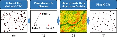
For areas with high-density GCPs (i.e. PSs; Figure 3a), we discard some of them to guarantee the remaining points uniformly distributed (Li, Zhang, and Qiu 2019) by taking into account the point density and the slope priority. In this process named GCP thinning, we first calculate the distance between each pair of candidate GCPs (Figure 3b) and examine the distribution of point density within the study area according to the number of adjacent points. Considering the distance between points and the number of points within local areas, we select suitable GCPs from the candidates and ensure their distribution is as dispersed and uniform as possible. Further, the slope (Figure 3c) of each GCP iscalculated to compare with its neighbors, where points with a lower slope arereserved when the GCP and neighbors have asimilar density. When two or more GCPs have similar slopes, we randomly select some of them from the candidates.

Figure 3. The workflow of the GCP thinning process.

The Average Nearest Neighbor (ANN) metric is applied to analyze the distribution of GCPs before and after thinning. This metric is based on the average distance from each GCP to its nearest neighboring GCP. The observed average distance (NNObserved) is calculated by the distance between each GCP and its nearest neighbor GCP. The z-score is a measure of statistical significance indicating whether or not the GCPs are randomly distributed. At the 99% confidence level, if the z-score is larger than 2.58 the GCPs are dispersed, and if the z-score is smaller than −2.58 the GCPs are clustered (Maguire, Batty, and Goodchild 2005).

2.3. The three-stage assessment

We propose a three-stage assessment method for evaluating the selected GCPs and generated DEMs (Figure 2c). The first stage verifies the phase and intensity of the selected GCPs. The selected GCPs are considered valid at this stage if their interference phases are around 0 rad and simultaneously their intensities are higher by 5 times than the averaged-intensity in the same image (Samsonov and Tiampo 2011). The second stage compares the elevations of the selected GCPs and the reference DEMs, where the GCPs with RMSE below 10 m for flat areas and 20 m for hilly areas are considered useful in InSAR processing (Braun 2021). The third stage compares external high-accuracy DEMs with the InSAR DEM generated by the auto-PS-GCP and auto-PS-GCP-Thin methods.

3. Materials

3.1. Study areas and datasets

Three study areas in plains, hilly areas, and mountainous areas (Figure 4) were selected to test our new auto-PS-GCP and auto-PS-GCP-Thin methods. The plain area is Beijing Downtown (Figure 4b) located in the North China Plain, the hilly area is Pingliang (Figure 4c) located in the loess hills of Gansu Province, and the mountainous area is Zhangjiakou (Figure 4d) located in the Yanshan Mountain. The Beijing downtown area is about 500 km², and the Pingliang and Zhangjiakou areas are both about 600 km². The vegetation in the three areas is not abundant, effectively reducing the side impacts of vegetation cover on interferometry. For different geomorphic areas, Table 1 shows 24 scenes of Sentinel-1A IW mode SLC data of ascending pass having 5m×20 m resolution with VV polarization (scihub.copernicus.eu). We used the POD Precise Orbit Ephemerides (slqc.asf.alaska.edu) to correct the orbit parameters for pre-processing the SLC data.

Figure 4. The study areas with three types of terrain conditions. (a) A DEM map of China, (b) the Beijing Downtown in plain areas, (c) Pingliang in hilly areas, and (d) Zhangjiakou in mountainous areas. The base map of (b-d) is the true color composite of Landsat-8 OLI images.

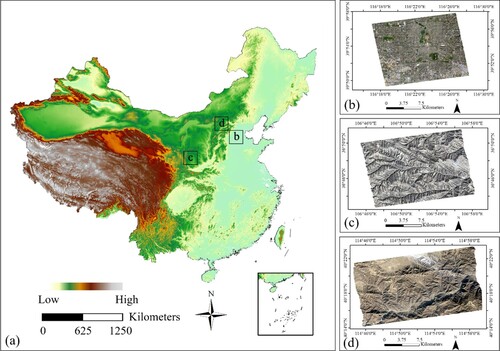
Table 1. The Sentinel-1A SAR images used in this study.

Series number	Acquisition date		Series number	Acquisition date
	Mountain/Plain	Hill		Mountain/Plain	Hill
1	2019.07.09	2019.06.28	13	2020.05.04	2020.04.11
2	2019.08.02	2019.07.22	14	2020.05.28	2020.05.05
3	2019.08.26	2019.08.15	15	2020.06.21	2020.05.29
4	2019.10.01	2019.09.08	16	2020.07.15	2020.06.22
5	2019.10.25	2019.10.02	17	2020.08.08	2020.07.16
6	2019.11.18	2019.10.26	18	2020.09.01	2020.08.09
7	2019.12.12	2019.11.19	19	2020.09.25	2020.09.02
8	2020.01.05	2019.12.13	20	2020.10.19	2020.09.26
9	2020.01.29	2020.01.06	21	2020.11.12	2020.10.20
10	2020.02.22	2020.01.30	22	2020.12.06	2020.11.13
11	2020.03.17	2020.02.23	23	2020.12.30	2020.12.07
12	2020.04.10	2020.03.18	24	2021.01.23	2020.12.31

The reference DEMs with finer spatial resolutions were derived from the PALSAR sensor of the Advanced Land Observing Satellite-1 project (ALOS) of the Japan Aerospace Exploration Agency (search.asf.alaska.edu). The terrain resolution in Fine Beam Single polarization mode is 12.5 m, and the vertical resolution is 12 m. The ALOS DEM was also used to provide a geographic coordinate reference for geocoding the Sentinel-1A data and to remove the flattening effect. The SRTM DEM covering the test area and ICESat-2 laser altimetry points with high vertical accuracy were used as the benchmarks for accuracy assessment of the generated DEMs (Guth and Geoffroy 2021).

3.2. Data pre-processing

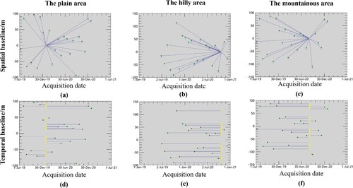
As indicated by the workflow of InSAR DEM generation (Figure 2a), the master images were selected considering both the temporal and spatial baselines. We selected the master SAR image from 24 scenes of Sentinel-1A data (within 18 months) for each study area (Figure 5). The other 23 SAR images are slaves, which then generated 23 time-series interferograms for each study area. For the plain and mountainous areas, the averaged spatial baselines are respectively 48.54 and 47.51 m, and the temporal baselines of the two study areas are appropriate (Pawluszek-Filipiak and Borkowski 2020). Particularly, for the hilly area, the spatial baselines with an average of 48.2428 m are appropriate for generating the interferograms (Wang, Tang, and Li 2018); however, some of the temporal baselines are as long as 479 days, which could reduce the coherence of the interferograms.

Figure 5. The spatial baselines (a-c) and temporal baselines (d-f) for the three study areas. The acquisition dates of the master images are Jan 29, 2020 for the plain area, Oct 20, 2020 for the hilly area, and Sep 1, 2020 for the mountainous area. The yellow dots denote the master images and the green dots denote the slave images.

After registering the master and slave images, the interference processing was performed to generate the interferograms and the Goldstein filtering method was performed to filter the interferograms. The filtered interferograms were then phase unwrapped by the minimum cost flow method to derive the true phase corresponding to the terrain information. To improve the interferograms, orbit refinement and reflattening were performed by importing the selected GCPs. Since the GCP selection was performed in the geographic coordinate system, we converted the GCPs into the slant-range coordinate system for InSAR DEM generation. Finally, the DEMs of the three study areas were successfully generated through phase-elevation conversion and geocoding.

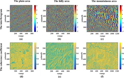
Figure 6 shows the typical interferograms and coherence maps that were derived based on SAR images with a revisiting period of 24 days. The coherence maps and the interferograms jointly reflect the undulating topography. For these maps, higher correlation coefficients and clearer interference fringes indicate higher credibility of the interference results. For the plain (Figure 6a and d) and mountainous areas (Figure 6c and f), the interference fringes are clear and most areas yield high coherence. The overall coherence is lower in the hilly area than in the other two areas, but most areas show clear interference fringes (Figure 6b) and high coherence (Figure 6e). Therefore, the InSAR DEM can be effectively generated using these interferograms and coherence maps.

Figure 6. The interferograms (a-c) and coherence maps (d-f). The interference pairs were generated using the master image on Jan 29, 2020 and the slave image on Feb 22, 2020 for the plain area, the master on Oct 20, 2020 and the slave on Nov 13, 2020 for the hilly area, and the master on Sep 1, 2020 and the slave on Sep 25, 2020 for the mountainous area.

4. Experiments and results

4.1. The selected GCPs based on the auto-PS-GCP method

Before geocoding the unwrapped interferometric phase, the GCPs were selected for orbit refinement and reflattening to improve the phase. We first assigned the thresholds for the features (e.g. coherence), then the auto-PS-GCP method automatically selected the GCPs for each study area by the coherence, averaged-amplitude, ADI, terrain slope, and distribution of GCPs. Table 2 shows that the low-thresholds of the coherences (γ_pix-thd1) were defined as 0.4 according to earlier studies (Foroughnia et al. 2019). The averaged-amplitude thresholds (A_img-thd) were the minimum A_img (Wang 2020). The ADI thresholds (A_pix-disp-thd) were assigned as 0.15, 0.20, and 0.25 for the three areas (Crosetto et al. 2016). The high-thresholds of the coherences (γ_pix-thd2) were then defined to select more useful GCPs from the above PSCs (Zhang et al. 2019). In the plain study area, γ_pix-thd2 was assigned as high as 0.98 in the Beijing downtown to derive the suitable number of GCPs. Finally, the GCPs with slopes lower than 15° (Szabó, Singh, and Szabó 2015) were selected to ensure that these points were derived in flat areas. The GCPs derived using auto-PS-GCP show relatively stronger clustering, which was reduced using the thinning method.

Table 2. The thresholds defined in auto-PS-GCP for the three study areas and the distribution assessment of the GCPs.

Criterion/Method		Threshold and assessment
		Plain	Hill	Mountain
γpix-thd1		0.40	0.40	0.40
Aimg-thd		The minAimg	The minAimg	The minAimg
Apix-disp-thd		0.15	0.20	0.25
γpix-thd2		0.98	0.93	0.80
SLOPEthd		15°	15°	15°
manual	Number	40	26	58
	NNObserved	0.0118	0.0193	0.0172
	z-score	4.8925	4.6685	4.6782
auto-PS-GCP	Number	135	89	213
	NNObserved	0.0032	0.0030	0.00270
	z-score	−9.2943	−10.1678	−13.5136
auto-PS-GCP-Thin	Number	40	26	58
	NNObserved	0.0139	0.0111	0.0132
	z-score	8.3903	1.4991	2.2490

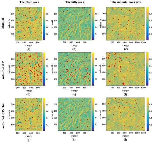
Figure 7 compares the GCP distribution of the manual, auto-PS-GCP, and auto-PS-GCP-Thin methods. The number of GCPs is the same for the manual and auto-PS-GCP-Thin methods, facilitating their comparison of distribution. The Beijing downtown has many unchanged scatterers, leading to the large amount of GCPs in the plain area (Figure 7d). After performing thinning to the GCPs from auto-PS-GCP (Figure 7d-f), the points of auto-PS-GCP-Thin show more reasonable distribution (Figure 7g-i); specifically, the number of GCPs in the plain, hilly, and mountainous areas are reduced by about 70%. Table 2 shows that the GCPs by manual and auto-PS-GCP-Thin are dispersed distribution because their z-score is larger than 2.58 while the GCPs by auto-PS-GCP are clustered distribution because their z-score is smaller than −2.58. The thinning processing has converted the automatically selected GCPs from clustering to dispersion, thus improving the GCP distribution.

Figure 7. The selected GCPs overlaid on the corresponding coherence maps, where for the three study areas, (a-c) indicate the manual selection, (d-f) indicate the auto-PS-GCP selection, and (g-i) indicate the auto-PS-GCP-Thin selection. The red dots denote the selected GCPs.

4.2. The first-stage assessment of the selected GCPs

To assess the intensity and phase (the first-stage assessment), we performed interference processing for all SAR image pairs and presented the results of an image pair only for each study area due to the page limitation (Table 3). Because of the short time interval between each image pair, there are only minor effects of deformation and minor influences of external factors such as weather conditions. Table 3 compares the averaged intensity between the entire SAR image and the GCPs selected by the three methods. The averaged intensity is higher for the GCPs selected by auto-PS-GCP and auto-PS-GCP-Thin than for the entire SAR image. The averaged intensity of the GCPs by manual is slightly different from that of the entire image. For example, in the plain area, Table 3 shows that the averaged intensity of the GCPs by manual is twice that in the entire image, and those of the GCPs by auto-PS-GCP and auto-PS-GCP-Thin are much greater, more than 20 times of the entire image. Similar improvements in the averaged intensity were found for the hilly and mountainous areas. These indicate that the GCPs selected by the two proposed methods have strong scattering.

Table 3. The First-stage assessment of the GCPs regarding the averaged intensity.

Area	Master	Slave	Method/Image	Number of GCPs	Averaged intensity (dB)
Plain	2019.08.02	2019.07.09	The entire image	N/A	3.2329
			Manual	40	8.2474
			auto-PS-GCP	135	76.4303
			auto-PS-GCP-Thin	40	59.3267
Hill	2019.07.22	2019.07.28	The entire image	N/A	0.1743
			Manual	26	0.2472
			auto-PS-GCP	89	2.3366
			auto-PS-GCP-Thin	26	2.9514
Mountain	2019.08.02	2019.07.09	The entire image	N/A	0.2799
			Manual	58	0.2708
			auto-PS-GCP	213	1.6894
			auto-PS-GCP-Thin	58	1.5585

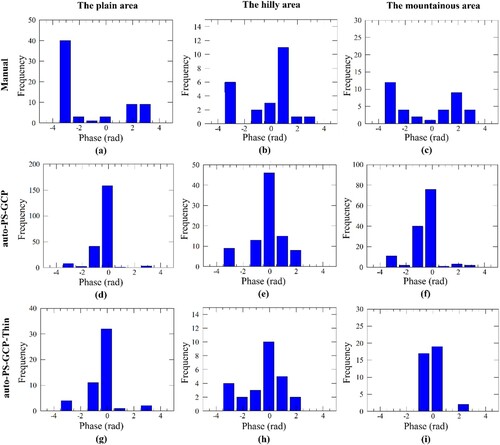
Figure 8 shows the phase histograms for the above interference pairs. The phases of the GCPs by manual do not display consistent distribution across the three study areas (Figure 8a-c), while the phases of the GCPs by auto-PS-GCP and auto-PS-GCP-Thin show high frequency near 0 rad (Figure 8d-i). This indicates that the GCPs selected by auto-PS-GCP and auto-PS-GCP-Thin have good phase stability, proving the effectiveness and feasibility of the two methods. For auto-PS-GCP-Thin, the selected GCPs not only have high scattering and phase stability but also yield nearly dispersed distribution in flat regions, indicating the usability of these GCPs in the consequent InSAR DEM generation.

Figure 8. The phase histogram-based GCPs by manual (a-c), auto-PS-GCP (d-f), and auto-PS-GCP-Thin (g-i).

4.3. The second-stage assessment of the selected GCPs

The GCPs selected by the three methods were then imported into the InSAR processing for refinement and reflattening. Figure 9(a-i) shows the DEMs generated using InSAR with the selected GCPs. We then compared the elevation of the GCPs in the generated DEMs with the homonymous points in the reference DEMs by calculating their RMSEs (Table 4). The RMSE of these GCPs by auto-PS-GCP-Thin is the smallest, which shows the best performance; whereas, the RMSE of the GCPs by auto-PS-GCP is greater than by manual, indicating the side effects of the GCP clustering on the DEM generation. In other words, greater aggregation of GCPs may lead to a reduction in the DEM accuracy. Although manual and auto-PS-GCP-Thin produced the same number of GCPs, the generated InSAR DEM is better when using GCPs with strong scattering and nearly dispersed distribution. These indicate the good performance of the proposed auto-PS-GCP-Thin method.

Figure 9. The generated DEMs related to three GCP selection methods where (a-c) denote the DEMs related to manual, (d-f) denote the DEMs related to auto-PS-GCP, (g-i) denote the DEMs related to auto-PS-GCP-Thin, and (j-l) denote the external SRTM DEMs.

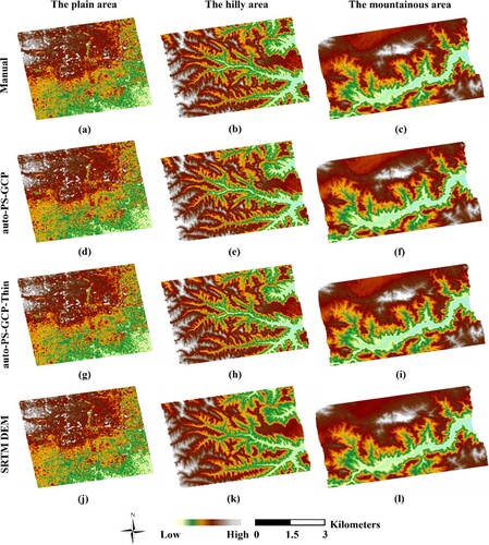
Table 4. The RMSE between the GCPs in DEMs related to each of the three methods and the homonymouspoints in the corresponding reference DEM.

Method	RMSE (m)
	Plain	Hill	Mountain
Manual	8.54	17.32	14.33
auto-PS-GCP	9.21	20.08	21.44
auto-PS-GCP-Thin	6.56	14.20	12.82

4.4. The third-stage assessment of the generated DEMs

To evaluate the DEM accuracy, we used the SRTM DEM with a 30 m resolution as the external DEM (Figure 9j-l) and generated 100 random points that are shown in the difference maps between the generated DEMs by auto-PS-GCP-Thin and the external SRTM DEMs (Figure 10a-c). The elevations of these random points were extracted from these two types of DEMs, and a comparison was performed to report the accuracy (Table 5). The DEMs related to the GCPs by auto-PS-GCP-Thin have the highest accuracy for all three study areas. Due to the influence of GCP aggregation, the DEMs related to the auto-PS-GCP have the lowest accuracy for all three study areas. The accuracy comparison before and after thinning shows that the GCPs after thinning have led to much better DEMs, which is attributed to the GCPs having strong scattering and stable phase. Among the three geomorphic types, the plain area has the best accuracy while the hilly area is not so good; in terms of methods, auto-PS-GCP-Thin performs the best for all three study areas as confirmed by the second-stage assessment.

Figure 10. The DEM accuracy evaluation using SRTM DEM and ICESat-2, where (a-c) denotethat the selected points areoverlaid on the difference maps between the generated DEMs and the SRTM DEMs, and (d-f) denote that the ICESat-2 laser altimetry points areoverlaid on the DEMs by auto-PS-GCP-Thin.

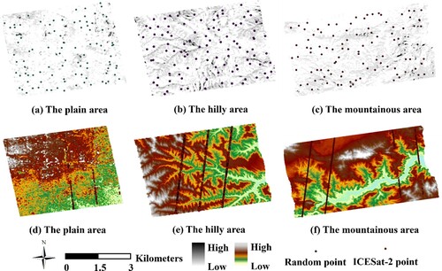
Table 5. The differences between the generated DEMs and the external elevations.

Area	Method	The differences (m) at different levels
		<1m	<3m	<5m	<10m	<20m	<30m	Total	RMSE for SRTM	RMSE for ICESat-2
Plain	Manual	15	10	16	29	25	5	100	6.16	9.64
	auto-PS-GCP	15	12	20	26	24	3	100	5.94	9.02
	auto-PS-GCP-Thin	18	15	14	28	21	4	100	4.71	7.88
Hill	Manual	8	3	3	20	18	21	100	17.96	23.91
	auto-PS-GCP	6	0	1	28	14	13	100	23.87	25.20
	auto-PS-GCP-Thin	9	3	1	24	19	27	100	14.97	19.01
Mountain	Manual	7	3	6	19	27	22	100	17.17	22.84
	auto-PS-GCP	7	3	8	15	21	13	100	19.53	28.34
	auto-PS-GCP-Thin	8	9	5	16	21	35	100	13.27	18.13

In addition, we chose the ICESat-2 laser altimetry points covering the study areas to perform further accuracy assessment. The ICESat-2 points are overlaid on the DEMs generated based on auto-PS-GCP-Thin (Figure 10d-f). Compared to the assessment using SRTM DEM, the elevation accuracies computed using ICESat-2 are lower by an average of 4.49 m, where the manual method shows the highest difference of 5.0 m, the auto-PS-GCP method yields a middle difference of 4.4 m, and the auto-PS-GCP-Thin method yields the least difference of 4.0 m (Table 5). Meanwhile, the mountainous area yields the highest difference of 4.86 m and the plain area yields the least difference of 3.18 m. Overall, both SRTM DEM and ICESat-2 indicate that the auto-PS-GCP-Thin method is the best among the three methods and the plain area has the best accuracy among the three geomorphic types.

5. Discussion

5.1. The strategy of GCP selection

Selected pixels with stable phase and strong scattering are essential for orbit refinement and reflattening in InSAR. We proposed an automatic selection method to extract GCPs for refinement and reflattening based on PSs. The GCP selection was conducted considering the coherence, amplitude, ADI, and terrain slope. In particular, the clustering GCPs was thinned considering the point density and slope priority. These selected GCPs were imported into the InSAR processing to generate DEMs with three case study areas in plain, hilly, and mountainous regions. The methods and results were evaluated using a three-stage assessment method. The first-stage showed that the GCPs by the new methods possess good phase stability and strong intensity, the second-stage showed that the RMSEs of the GCPs by auto-PS-GCP-Thin are about 6∼12 m for different terrain areas, and the third-stage showed that the RMSEs of the generated DEMs by auto-PS-GCP-Thin are about 4∼15 m for different areas.

The definition of thresholds is crucial to GCP selection and we considered five aspects related to SAR images, coherence, amplitude, ADI, terrain conditions, and GCP distribution (Bayer, Schmidt, and Simoni 2017; Khorrami et al. 2019). The low-threshold of coherence was acknowledged as 0.4 to remove low coherence points, and the minimum averaged-amplitude was acknowledged as the threshold to remove points exhibiting falsely high coherence. The ADI threshold was usually assigned lower than 0.25 to ensure the consistency of the selected points in long time series (Crosetto et al. 2016). In this study, we defined the ADI threshold as 0.15∼0.25 to extract stable GCPs. A high-threshold of coherence was then defined to further identify permanent facilities as GCPs from previously selected points, where the threshold was commonly assigned about 0.90∼0.98 (Giardina et al. 2019). These thresholds are well applicable in different areas and our contribution is the integration of accurately identifying high-quality GCPs. In addition, the GCP selection is also influenced by the SAR imaging overlay and shadow effect, which is highly related to the terrain slope. We defined the slope threshold as 15° to further identify the GCPs in the flat areas by referring to earlier studies of terrain classification (Drăguţ and Blaschke 2008). Integrating slope into GCP selection can remove points influenced by overlay and shadow effect that has not well been addressed in the literature (Bayer, Schmidt, and Simoni 2017).

The GCP selection is jointly affected by phase stability, scattering intensity, and GCP distribution. The GCPs selected by auto-PS-GCP have stable phase and high scattering intensity while those by manual showed dispersed (i.e. more suitable) distribution (c.f. Figure 7 and 8). According to the second-stage assessment, in the plain area, the GCP RMSE by auto-PS-GCP was 9.21 m, that of the manual was 8.54 m, and that of auto-PS-GCP-Thin was only 6.56 m (c.f. Table 4). The results indicate that the GCP distribution is a more important factor affecting the consequent InSAR DEM generation. The averaged intensity of the GCPs was lower by auto-PS-GCP-Thin than by auto-PS-GCP (c.f. Table 3), which could be caused by the deletion of some of the high-intensity points that were aggregated in a very small area. These two methods yielded similar summary statistics, and their GCPs’ averaged scattering intensities were far greater than that of the manual.

To select GCPs, scientists also used a common strategy by setting a uniform grid (here we name this method as UniGrid) with an empirical pixel interval then weighting the observations using indexes like coherence (Wegnüller et al. 2016). For example, the GAMMA software uses the coherence mask to extract GCPs, and selects appropriate number of GCPs in range and azimuth by setting a predefined pixel interval (AG 2010). The UniGrid method uses only a single image while our auto-PS-GCP-Thin considers the stability and intensity of GCPs. This suggests that the former identifiesboth short-term (i.e. a revisiting period) and long-term (e.g. months to years) persistent GCPs while auto-PS-GCP-Thin directly identifies long-term persistent GCPs. The UniGrid method needs to traverse all evenly divided grids and then calculate the weights of all pixels according to the predefined indexes. After traversing, the UniGrid filters out a certain number of GCPs that meet the requirements. In contrast, the auto-PS-GCP-Thin method adopts a layered approach to set different thresholds according to indexes such as coherence and amplitude. Most of the pixels that do not meet the threshold of the first layer are eliminated firstly, then all steps are performed on the basis of the previous step (c.f. Figure 2). As the algorithm progresses, the number of pixels that need to be traversed and removed drastically reduces, and therefore the computation time. Compared to UniGrid, auto-PS-GCP-Thin may yield more limitations in the application, but it can ensure the stability of the selected GCPs that are suitable for more images. Particularly, it is the first time the thinning method was proposed to choose more suitable GCPs from a lot of candidates, improving the GCPs quality and the generated DEMs. In addition, auto-PS-GCP-Thin has been proved robust in the three areas with different terrain conditions.

5.2. Assessment of the generated DEMs

In this study, we chose Sentinel-1A with anarrow orbit cube as the experimental data (Braun 2021; Braun, Höser, and Delgado Blasco 2021) because of its popularity in generating DEMs worldwide. The baseline of Sentinel-1A is small thus it is difficult to derive high accuracy DEMs (Nonaka et al. 2019). Because Sentinel-1 has relatively accurate orbital data, the purpose of selecting GCPs with high intensity and stable phase is to correct the phase offset to improve the DEM accuracy. There are two reasons for the phase offset: (1) the influence of the flattening effect, and (2) the error of the baseline parameters. Our results show substantial improvement in DEM generation using Sentinel-1A images, thus the proposed method can also be utilized in applications using other SAR images such as China's Gaofen-3, whose orbit accuracyis lower than that of Sentinel-1A (Wang et al. 2019).

In the three cases using the Sentinel-1A images, the terrain conditions have a substantial impact on the InSAR DEM accuracy (Sosnovsky, Kobernichenko, and Vinogradova 2019). Our assessment with SRTM DEM and ICESat-2 indicates that all three methods haveled to the best accuracies in the plain area where auto-PS-GCP-Thin performed the best with the elevation accuracy of 4.71 m evaluated by SRTM DEM and 7.88 m evaluated byICESat-2. Whereas, this method yielded an accuracy of 14.97 m evaluated by SRTM DEM and 19.01 m evaluated byICESat-2 in the hilly area, reporting the lowest in all three areas (c.f. Table 5). In addition, the coherence of the hilly area was the weakest in all three areas (c.f. Figure 6), correspondingly the selected GCPs were the fewest. Our new auto-PS-GCP-Thin method can generate preferable accuracy of DEMs when compared to other methods applied elsewhere (Mohammadi et al. 2020). For example, a case of the DEM generation in Bushehr city showed an RMSE of 18.53 m using the Sentinel-1A data (Ghannadi et al. 2020).

To well compare the three methods, we applied a comprehensive three-stage assessment method to calculate the GCPs’ phase and intensity, RMSE, and the accuracy of DEMs. We used both SRTM and ICESat-2 to evaluate the DEM accuracy in the third-stage assessment to inspect the reliability (Bhardwaj 2021). For the manual selection, although its GCPs are useful, the selection is somewhat variable because it depends on human decision, the RMSE is different each time consequently. The auto-PS-GCP-Thin considers the phase stability, scattering intensity, terrain slope, and the GCP distribution, hence the results are consistent and can be applied to a variety of situations. Our results indicate that interference processing using GCPs selected based on PSs can generate high-precision DEMs (c.f. Table 5). The determination of PSs commonly needs many images of a long-term sequence to guarantee stability, and the PSs can not only be used for settlement monitoring but also are very useful (as input GCPs) to generate DEMs through interference processing. Also, it proves that the points with strong scattering and high stability characteristics play a useful role in the InSAR orbit refinement and reflattening processing.

6. Conclusions

High-quality GCPs for orbit refinement and reflattening are essential for InSAR DEM generation. The GCPs can be extracted from PSs that are usually consistent ground targets maintaining phase stability and strong scattering intensity in long time-series images. This study proposed two GCP selection methods (i.e. auto-PS-GCP and auto-PS-GCP-Thin), which were tested in three areas of plains, hills, and mountains. The low-coherence and averaged-amplitude that indicate the scattering intensity was firstly utilized to derive PSCs. The ADI and high-coherence were then adopted to extract higher quality PSs with stable phase and high coherence from the above PSCs, and the terrain slope was further considered to delete points with high-slope. Finally, a point thinning method was proposed to correct the distribution of the GCPs (i.e. PSs) by discarding some points that were aggregated in a very small area, and the quality and suitability of the selected GCPs are evaluated using metrics such as ANN. The results show that the DEM accuracy was affected by both the properties and the distribution of the GCPs. When SRTM DEM was used as the external DEM, the DEM accuracy related to the auto-PS-GCP-Thin was improved by about 20%∼30% for different areas compared to the manual, where the best performance in plain areas with the DEM accuracy was about 4.71 m. In addition, the auto-PS-GCP-Thin improved the DEM accuracy by about 20%–40% compared to the auto-PS-GCP. Further assessment accuracies with ICESat-2 laser altimetry points were lower by an average of 4.49 m than those of SRTM DEM, where auto-PS-GCP-Thin and the plain area also showed the highest accuracies.

Our method of GCP selection comprehensively considered the influencing factors of phase stability, scattering intensity, terrain slope, and GCP distribution. The three comparable case studies showed that auto-PS-GCP-Thin is a reliable method in InSAR DEM generation. It is concluded that the proposed method is effective in various areas with different terrain conditions. Limitations such as the definition of multiple thresholds exist in this study, and future work should consider the automatic search of these thresholds using deep learning and high-performance computation methods.

Data availability statement

The data sets are freely available at https://figshare.com/s/cb2422704fa533d3df37.

Disclosure statement

No potential conflict of interest was reported by the author(s).

Additional information

Funding

Supported by the National Key R&D Program of China (2021YFB3900105-2) and the National Natural Science Foundation of China (42071371).

References

- AG, G.R.S. 2010. Interferometric SAR Processor j ISP. Documentation j User, s Guide. Vers 1.
- Bayer, B., D. Schmidt, and A. Simoni. 2017. “The Influence of External Digital Elevation Models on PS-InSAR and SBAS Results: Implications for the Analysis of Deformation Signals Caused by Slow Moving Landslides in the Northern Apennines (Italy).” IEEE Transactions on Geoscience and Remote Sensing 55: 2618–2631.
- Berardino, P., G. Fornaro, R. Lanari, and E. Sansosti. 2002. “A New Algorithm for Surface Deformation Monitoring Based on Small Baseline Differential SAR Interferograms.” IEEE Transactions on Geoscience & Remote Sensing 40: 2375–2383.
- Bhardwaj, A. 2021. “Investigating the Terrain Complexity from ATL06 ICESat-2 Data for Terrain Elevation and Its Use for Assessment of Openly Accessible InSAR Based DEMs in Parts of Himalaya’s.” Engineering Proceedings 10: 65.
- Bhardwaj, A., K. Jain, and R. S. Chatterjee. 2019. “Generation of High-Quality Digital Elevation Models by Assimilation of Remote Sensing-Based DEMs.” Journal of Applied Remote Sensing 13: 044502.
- Braun, A. 2021. “Retrieval of Digital Elevation Models from Sentinel-1 Radar Data–Open Applications, Techniques, and Limitations.” Open Geosciences 13: 532–569.
- Braun, A., T. Höser, and J. M. Delgado Blasco. 2021. “Elevation Change of Bhasan Char Measured by Persistent Scatterer Interferometry Using Sentinel-1 Data in a Humanitarian Context.” European Journal of Remote Sensing 54: 109–126.
- Chen, X., J. Peng, and H. Yang. 2017. “Orbital Error Modeling and Analysis of Spaceborne InSAR, 2017 SAR in Big Data Era: Models, Methods and Applications (BIGSARDATA).” IEEE, 1–6.
- Child, S. F., L. A. Stearns, L. Girod, and H. H. Brecher. 2021. “Structure-From-Motion Photogrammetry of Antarctic Historical Aerial Photographs in Conjunction with Ground Control Derived from Satellite Data.” Remote Sensing 13: 21.
- Chureesampant, K., and J. Susaki. 2014. “Automatic GCP Extraction of Fully Polarimetric SAR Images.” IEEE Transactions on Geoscience and Remote Sensing 52: 137–148.
- Crosetto, M., O. Monserrat, M. Cuevas-González, N. Devanthéry, and B. Crippa. 2016. “Persistent Scatterer Interferometry: A Review.” ISPRS Journal of Photogrammetry and Remote Sensing 115: 78–89.
- Crosetto, M., O. Monserrat, G. Luzi, M. Cuevas, and N. Devanthéry. 2015. “Deformation Monitoring Using Ground-Based SAR Data.” In Engineering Geology for Society and Territory, 5 vols., 137–140. Springer.
- Dinh, H. T. M., H. Ramon, and R. Fabio. 2020. “Radar Interferometry: 20 Years of Development in Time Series Techniques and Future Perspectives.” Remote Sensing 12: 1364.
- Drăguţ, L. D., and T. Blaschke. 2008. “Terrain Segmentation and Classification Using SRTM Data.” In Advances in Digital Terrain Analysis, 141–158. Springer.
- Du, Y., G. Feng, Z. Li, X. Peng, J. Zhu, and Z. Ren. 2017. “Effects of External Digital Elevation Model Inaccuracy on StaMPS-PS Processing: A Case Study in Shenzhen, China.” Remote Sensing 9: 1115.
- Du, Q. S., G. Y. Li, W. L. Peng, Y. Zhou, M. T. Chai, and J. M. Li. 2021. “Acquiring High-Precision DEM in High Altitude and Cold Area Using InSAR Technology.” Bulletin of Surveying and Mapping 0: 44–49.
- Du, Y., S. Yang, and H. Shi. 2010. “Study on Accurate Estimation of Baseline Parameters of Space-Borne InSAR Based on GCPs.” In 2010 18th International Conference on Geoinformatics, IEEE, 1–4.
- Ferretti, A., C. Prati, and F. Rocca. 2001. “Permanent Scatterers in SAR Interferometry.” IEEE Transactions on Geoscience and Remote Sensing 39: 8–20.
- Foroughnia, F., S. Nemati, Y. Maghsoudi, and D. Perissin. 2019. “An Iterative PS-InSAR Method for the Analysis of Large Spatio-Temporal Baseline Data Stacks for Land Subsidence Estimation.” International Journal of Applied Earth Observation and Geoinformation 74: 248–258.
- Ghannadi, M. A., S. Alebooye, M. Izadi, and A. Moradi. 2020. “A Method for Sentinel-1 DEM Outlier Removal Using 2-D Kalman Filter.” Geocarto International, 1–15.
- Giardina, G., P. Milillo, M. J. DeJong, D. Perissin, and G. Milillo. 2019. “Evaluation of InSAR Monitoring Data for Post-Tunnelling Settlement Damage Assessment.” Structural Control and Health Monitoring 26: e2285.
- Guth, P. L., and T. M. Geoffroy. 2021. “LiDAR Point Cloud and ICESat-2 Evaluation of 1 Second Global Digital Elevation Models: Copernicus Wins.” Transactions in GIS 25: 2245–2261.
- Jauvin, M., Y. Yan, and E. Trouvé. 2017. “Combined Use of Spaceborne SAR Interferometry and In-situ Measurements for Glacier Monitoring in Mountain Areas.” In 2017 IEEE International Conference on Computational Intelligence and Virtual Environments for Measurement Systems and Applications (CIVEMSA), IEEE, 199–204.
- Khorrami, M., B. Alizadeh, E. Ghasemi Tousi, M. Shakerian, Y. Maghsoudi, and P. Rahgozar. 2019. “How Groundwater Level Fluctuations and Geotechnical Properties Lead to Asymmetric Subsidence: A PSInSAR Analysis of Land Deformation Over a Transit Corridor in the Los Angeles Metropolitan Area.” Remote Sensing 11: 377.
- Li, Z., G. Liu, and X. Ding. 2006. “Exploring The Generation Of Digital Elevation Models from Same-Side Ers Sar Images: Topographic And Temporal Effects.” Photogrammetric Record 21: 124–140.
- Li, P., K. Sun, D. Li, H. Sui, and Y. Zhang. 2017. “An Emergency Georeferencing Framework for GF-4 Imagery Based on GCP Prediction and Dynamic RPC Refinement.” Remote Sensing 9: 1053.
- Li, F., Y. Zhang, and X. Qiu. 2019. “An Approach for Spaceborne InSAR DEM Inversion Integrated with Stereo-SAR Method.” In 2019 6th Asia-Pacific Conference on Synthetic Aperture Radar (APSAR), IEEE, 1–4.
- Liu, W., Q. Zhang, and Y. Zhao. 2020. “A Fuzzy Identification Method for Persistent Scatterers in PSInSAR Technology.” Mathematical Biosciences and Engineering 17: 6928–6944.
- Maguire, D. J., M. Batty, and M. F. Goodchild. 2005. GIS, Spatial Analysis, and Modeling. Esri Press.
- Marotti, L., A. Parizzi, N. Adam, and K. Papathanassiou. 2008. “Coherent vs. Persistent Scatterers: A Case Study.” In 7th European Conference on Synthetic Aperture Radar, VDE, 1–4.
- Mohammadi, A., S. Karimzadeh, S. J. Jalal, K. V. Kamran, H. Shahabi, S. Homayouni, and N. Al-Ansari. 2020. “A Multi-Sensor Comparative Analysis on the Suitability of Generated DEM from Sentinel-1 SAR Interferometry Using Statistical and Hydrological Models.” Sensors 20: 7214.
- Mu’amalah, A., I. M. Anjasmara, and M. Taufik. 2021. “Land Subsidence Monitoring in Cepu Block Area Using PS-Insar Technique.” In IOP Conference Series: Earth and Environmental Science, IOP Publishing, 012011.
- Müller, R., T. Krauß, M. Schneider, and P. Reinartz. 2012. “Automated Georeferencing of Optical Satellite Data with Integrated Sensor Model Improvement.” Photogrammetric Engineering & Remote Sensing 78: 61–74.
- Nonaka, T., T. Asaka, K. Iwashita, and F. Ogushi. 2019. “The Relationships Between Errors of DEM and the Height of Ambiguity of Sentinel-1.” In IGARSS 2019-2019 IEEE International Geoscience and Remote Sensing Symposium, IEEE, 1725–1728.
- Pan, B., and L. Liu. 2010. “Precise SAR Satellite Orbit Parameters Determination Based on Ground Control Points.” In 2010 18th International Conference on Geoinformatics, IEEE, 1–5.
- Pawluszek-Filipiak, K., and A. Borkowski. 2020. “Integration of DInSAR and SBAS Techniques to Determine Mining-Related Deformations Using Sentinel-1 Data: The Case Study of Rydułtowy Mine in Poland.” Remote Sensing 12: 242.
- Pepe, A., and F. Calò. 2017. “A Review of Interferometric Synthetic Aperture RADAR (InSAR) Multi-Track Approaches for the Retrieval of Earth's Surface Displacements.” Applied Sciences 7: 1264.
- Qu, S. B., Y. P. Wang, and H. Wen. 2011. “The PS Selection Method Using Temporal Information in PSDInSAR Technique.” Journal of Electronics & Information Technology 33: 381–387.
- Rosen, P. A., S. Hensley, I. R. Joughin, F. K. Li, S. N. Madsen, E. Rodriguez, and R. M. Goldstein. 2000. “Synthetic Aperture Radar Interferometry.” Proceedings of the IEEE 88: 333–382.
- Samsonov, S., and K. Tiampo. 2011. “Polarization Phase Difference Analysis for Selection of Persistent Scatterers in SAR Interferometry.” IEEE Geoscience and Remote Sensing Letters 8: 331–335.
- Shirani, K., and M. Pasandi. 2019. “Detecting and Monitoring of Landslides Using Persistent Scattering Synthetic Aperture Radar Interferometry.” Environmental Earth Sciences 78: 42.
- Sosnovsky, A., V. Kobernichenko, and N. Vinogradova. 2019. “The Problem of Quality Assessing for the Methods of Coherence Maps Calculation in InSAR Remote Sensing of the Earth Data Processing.” In Journal of Physics: Conference Series, IOP Publishing, 032023.
- Szabó, G., S. K. Singh, and S. Szabó. 2015. “Slope Angle and Aspect as Influencing Factors on the Accuracy of the SRTM and the ASTER GDEM Databases.” Physics and Chemistry of the Earth, Parts A/B/C 83-84: 137–145.
- Tian, W., Z. Zhao, J. Wang, T. Zeng, and Y. Deng. 2019. “GB-InSAR Interferogram Processing Method to Generate DEM Based on PS Technology.” The Journal of Engineering 2019: 6625–6628.
- Wang, J. F. 2020. “Application of a Permanent Scatterers Selection Method in GB-SAR Slope Monitoring Data Processing.” Science of Surveying and Mapping 45.
- Wang, Z., X. Tang, and T. Li. 2018. “Impact Analysis of InSAR Spatio-Temporal Baseline on DEM Accuracy.” Bulletin of Surveying and Mapping 61.
- Wang, J., W. Yu, Y. Deng, R. Wang, Y. Wang, H. Zhang, and M. Zheng. 2019. “Demonstration of Time-Series InSAR Processing in Beijing Using a Small Stack of Gaofen-3 Differential Interferograms.” Journal of Sensors 2019: 4204580.
- Wegmuller, U., C. Werner, A. Wiesmann, T. Strozzi, and M. Santoro. 2008. “Initial Assessment of the Applicability of TerraSAR-X for Repeat-Track Interferometry.” In IGARSS 2008-2008 IEEE International Geoscience and Remote Sensing Symposium, IEEE, II-529-II-532.
- Wegnüller, U., C. Werner, T. Strozzi, A. Wiesmann, O. Frey, and M. Santoro. 2016. “Sentinel-1 Support in the GAMMA Software.” Procedia Computer Science 100: 1305–1312.
- Xiang, X., J. Chen, H. Wang, L. Pei, and Z. Wu. 2019. “PS Selection Method for and Application to GB-SAR Monitoring of Dam Deformation.” Advances in Civil Engineering 2019: 1–15.
- Yadav, V. P., R. Prasad, R. Bala, and A. K. Vishwakarma. 2020. “An Improved Inversion Algorithm for Spatio-Temporal Retrieval of Soil Moisture Through Modified Water Cloud Model Using C-Band Sentinel-1A SAR Data.” Computers and Electronics in Agriculture 173: 105447.
- Zeng, T., T. Zhang, W. Tian, and C. Hu. 2015. “A Novel Subsidence Monitoring Technique Based on Space-Surface Bistatic Differential Interferometry Using GNSS as Transmitters.” Science China Information Sciences 58: 1–16.
- Zhang, J., G. Shu, X. Yuan, and P. Qiu. 2019. “The Extraction and Analysis of Kunming Ground Deformation Characteristics Based on PS-InSAR.” Science of Surveying and Mapping 1: 53–59.
- Zhang, X., Q. Zeng, J. Jiao, and J. Zhang. 2016. “Fusion of Space-Borne Multi-Baseline and Multi-Frequency Interferometric Results Based on Extended Kalman Filter to Generate High Quality DEMs.” ISPRS Journal of Photogrammetry and Remote Sensing 111: 32–44.
- Zhao, Z. 2016. “Methods on High-Accuracy DEM Extraction from Interferometric SAR in Sophisticated Terrain Areas.” Acta Geodaetica Et Cartographica Sinica 45: 1385.