An optimized hexagonal quadtree encoding and operation scheme for icosahedral hexagonal discrete global grid systems

ABSTRACT

Although research on the discrete global grid systems (DGGSs) has become an essential issue in the era of big earth data, there is still a gap between the efficiency of current encoding and operation schemes for hexagonal DGGSs and the needs of practical applications. This paper proposes a novel and efficient encoding and operation scheme of an optimized hexagonal quadtree structure (OHQS) based on aperture 4 hexagonal discrete global grid systems by translation transformation. A vector model is established to describe and calculate the aperture 4 hexagonal grid system. This paper also provides two different grid code addition algorithms based on induction and $ijk$ coordinate transformation. We implement the transformation between OHQS codes and geographic coordinates through the $ij$, $ijk$ and $IJK$ coordinate systems. Compared with existing schemes, the scheme in this paper greatly improves the efficiency of the addition operation, neighborhood retrieval and coordinate transformation, and the coding is more concise than other aperture 4 hexagonal DGGSs. The encoding operation based on the $ijk$ coordinate system is faster than the encoding operation based on the induction and addition table. Spatial modeling based OHQS DGGSs are also provided. A case study with rainstorms demonstrated the availability of this scheme.

KEYWORDS:

• Discrete global grid systems
• hexagon
• quadtree encoding

SUBJECT CLASSIFICATION CODES:

• include these here if the journal requires them

1. Introduction

With the development of technology in earth science, the era of big earth data has arrived (Guo et al. 2014; Guo 2017). To meet the challenges in transmitting, storing, processing, analyzing, managing, and sharing big earth data, advanced technology is required to make the data manageable and valuable (Guo et al. 2017). Discrete global grid systems (DGGSs) are gaining traction as data models for a digital earth framework designed for heterogeneous geospatial big data (Craglia et al. 2012; Goodchild 2018). Based on its infrastructure, which is superior to regular grids based on map projections (Bauer-Marschallinger, Sabel, and Wagner 2014; Lin et al. 2018), the DGGS will enable the integrated analysis of massive, multisource, multiresolution, multidimensional earth observation data (Yao et al. 2020).

DGGSs comprise a spatial reference system that uses a hierarchical tessellation of cells to partition and address the globe, which is considered a promising model for processing big earth data. The Open Geospatial Consortium (OGC) specified the core abstract specification and extension mechanisms for the DGGS (Purss et al. 2017). In the DGGS, the earth's surface is partitioned into a set of cell regions, where each region has a single point and unique code associated with it. Compared with traditional spatial data organization and application mode, the DGGS can avoid the large deformation caused by direct projection. The DGGS is more suitable for solving large-scale problems and efficient processing of multiresolution data because of its hierarchical and continuous structure. As a tool, the DGGS has been employed in multiple fields, such as geospatial data management (Shuang et al. 2016; Li et al. 2019; Li, Stefanakis, and Mcgrath 2020), ocean modeling (Lin et al. 2018), construction of global gazetteers (Adams 2017), global oil palm monitoring (Cheng et al. 2017), integrated environmental analytics (Robertson et al. 2020), and prediction of hate crimes (Jendryke and McClure 2021).

Compared with the DGGS based on the geographic coordinate system, the geodesic DGGS based on regular polyhedrons has equal-area cell regions and can avoid distortion from the equator to the poles, which has increased its popularity among many researchers (Sahr, White, and Jon Kimerling 2003). Different geodesic DGGSs may be characterized according to base polyhedrons, cell shape, aperture, cell indexing, and projections (Mahdavi-Amiri, Alderson, and Samavati 2015; Peterson 2016). The base polyhedrons used to approximate the earth can be partitioned into cells and projected onto a sphere by a projection method. The icosahedral Snyder projection is commonly used in geodesic DGGS research due to its equal-area property and low angular distortion (Snyder 1992; Kimerling et al. 1999; White 2000; Sahr 2008; Vince and Zheng 2009). In geodesic DGGSs, there are three common cell shapes: triangle (Dutton 1984, 1999; Iii, John, and Goldsman 2001; Zhao, Chen, and Li 2006), quadrilateral (Alborzi and Samet 2000; White 2000; Amiri, Bhojani, and Samavati 2013), and hexagon (Sahr, White, and Jon Kimerling 2003; Vince 2006; Vince and Zheng 2009; Tong et al. 2013; Wang et al. 2021). Compared with other cell shapes, hexagonal cells have advantages such as close packing and uniform adjacency, which are favorable for spatial analysis and data visualization (Sahr 2011; Ben et al. 2015). Three hierarchical spatial partitioning structures—apertures 3, 4, and 7 were utilized in hexagonal DGGSs. Most research on multiprecision hexagonal DGGSs has focused on apertures 3 and 4.

The core functionality of the DGGS is the indexing method that supports the rapid indexing of spatial data in the DGGS and the efficient calculation of spatial analysis. The indexing categorization of the DGGS includes hierarchy-based indexing, space-filling curve indexing, and axes-based indexing. Different indexing methods have different characteristics and can be converted among each other (Amiri, Samavati, and Peterson 2015). For hexagonal DGGSs, hierarchy-based indexing methods are primarily utilized in research and application. Sahr (2005, 2008, 2011) introduced the icosahedral modified generalized balanced ternary (MGBT) for indexing the DGGS. Peterson (Peterson 2011) proposed the PYXIS scheme to encode and index cells of the Icosahedral Snyder Equal Area Aperture 3 Hexagonal (ISEA3H) DGGS. Arithmetic and Fourier transforms for the PYXIS were analyzed by Vince and Zheng (Zheng 2007; Vince and Zheng 2009). Mocnik proposed an identifier scheme that encodes the geographic coordinates of the centroid of a cell on ISEA3H DGGS (Mocnik 2019). Two types of aperture 4hexagonal grid systems were combined to construct the hexagonal quaternary balanced structure (HQBS) (Tong et al. 2013). According to the characteristics of the aperture 4 hexagonal grid systems, Wang et al. designed the hexagon lattice quad tree (HLQT) structure (Wang et al. 2018; Wang et al. 2019).

Compared with the aperture 3 hexagonal grid, the partition structure of the aperture 4 hexagonal grid is simple and consistent, and its encoding operation is more efficient. The Aperture 4 DGGS is usually based on quad-tree encoding, but coding gaps and unique attribution problems will arise in the process of quad-tree encoding. The encoding cannot tile the whole plane because hexagonal grid subdivision is not nested at different levels. The method adopted by the HLQT was to construct the first symbol in the third resolution to the tile plane. The HLQT code consisted of the first symbol and subsequent digits, which caused a mismatch between the first symbol and subsequent digits (Wang et al. 2019). The calculation of the first symbol was more complicated. The HQBS adopts quadtree encoding, which combines two types of aperture 4 hexagonal discrete grid systems into a hierarchy, leading to complicated operation rules and the situation in which the code ‘regularization’ fails and needs to be returned and recalculated (Tong et al. 2013). The discrete global grid encoding operation usually constructs addition tables and addition rules, which are complex to build and computationally complex (usually $O\left(N^2\right)$, by means of induction. In practical applications, more emphasis is placed on the simplicity, usability and efficiency of encoding operations. The efficiency of the existing DGGS still cannot meet the actual needs. The significance of the global discrete grid is to provide a new management and analysis scheme for spatial data. However, current research hardly provides the expression methods and interfaces of traditional spatial data on the discrete global grid, which limits the application of the DGGS.

In this study, we establish the mathematical vector model of the aperture 4 hexagonal grid system, which is used to express and operate the hexagonal quadtree encoding, and design the encoding scheme of the Optimized Hexagonal QuadTree Structure(OHQS) by translation transformation. The scheme is extended to the icosahedron and sphere. In the encoding addition and neighborhood retrieval operations, in addition to constructing a set of addition rules similar to integer addition by means of induction, we also construct a set of addition rules based on $ijk$ coordinate transformation. The efficiency of the two addition rules is compared. In the transformation algorithm between DGGS code and geographic coordinates, we calculate the coordinates of the center point of the grid by converting the code to the $ij$ coordinate system. The location characteristics of the hexagonal center point in the $ijk$ coordinate system and $IJK$ coordinate transformation are employed to calculate and determine the hexagonal grid code where the point is located. The data conversion model from traditional spatial data (vector data and raster data) to a discrete global grid is also constructed. Multisource data, such as social media data and elevation data, are utilized to analyze the influences of the ‘Beijing 7.16’ rainstorm disaster.

2. Optimized hexagonal quadtree structure

2.1 Basic model of a dGGS

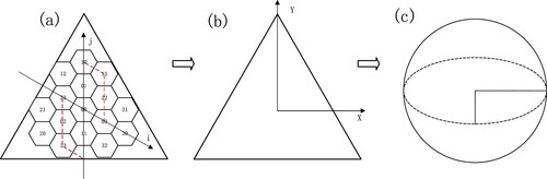
A geodesic DGGS is generally specified by a base polyhedron, orientation of the polyhedron relative to the earth, a hierarchical spatial partitioning method, projection, and assigning points to cells (Sahr, White, and Jon Kimerling 2003). To construct the spherical hexagonal grid system, first, nearly all existing hexagonal DGGSs should build a planar hexagonal grid system. Second, the polyhedral model is built based on the planar hexagonal grid system. Last, the polyhedral model is projected onto the sphere. In this study, we selected the Inverse Snyder Equal-Area Projection Aperture 4 Hexagon Discrete Global Grid System (ISEA4H DGGS) model, as shown in Figure 1, because aperture 4 hexagon hierarchy changes more regularly and the Icosahedral Snyder Equal-Area Projection has the most minor cell distortion (Kimerling et al. 1999; Mahdavi-Amiri, Alderson, and Samavati 2015).

Figure 1. Model of icosahedron DGGS

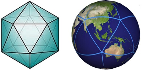
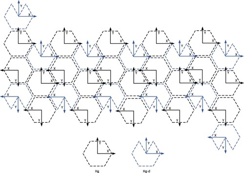
To construct the DGGS, the icosahedron is selected to approximate the earth, and the spherical discretization based on the earth is converted to discretization on the icosahedron. We determine the position of the icosahedron relative to the sphere by setting the vertices at the poles. The icosahedron is expanded, as shown in Figure 2. Referring to the discretization and encoding scheme in previous studies, the initial discretization is established in each triangular face of the icosahedron (Sahr 2008; Vince and Zheng 2009; Jin et al. 2018; Wang et al. 2019; Wang et al. 2021). We use Hg to indicate a complete hexagon, and Hg-d to indicate a hexagon with a triangle deleted. The two-dimensional coordinate axis $xy$ is used to identify the direction of hexagonal subdivision and encoding, and then the icosahedron is divided into 20 and 12 Hg-d, as shown in Figure 3. Note that the icosahedron is subdivided into 32 hexagons, and we just need to build a subdivision and encoding structure on each hexagon.

Figure 2. Diagram of initial hexagons on the unfolded icosahedron surface

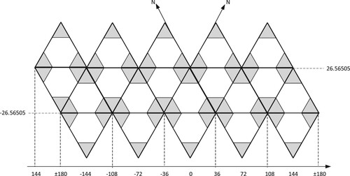
Figure 3. The direction of hexagonal subdivision and encoding

2.2 Design of optimized hexagonal quadtree structure encoding scheme

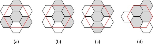
There are four types of hexagonal subdivisions in aperture 4 hexagonal DGGSs. As shown in Figure 4, the red hexagon representing parent cells is partitioned into four gray hexagons representing child cells. In this paper, the first structure (a) is selected as the basic hexagonal grid subdivision structure, which is symmetrical about the parent cell and has better geometric properties.

Figure 4. Four structures of hexagonal subdivisions

To facilitate the representation and calculation of the aperture 4 hexagonal DGGS, the lattice representing the center point of the planar hexagonal grid is defined to replace the grid. Vectors $u$ and $v$ in the two-dimensional Cartesian coordinate system are employed to describe the lattice. As illustrated in Figure 5 (right), the unit of the side length of the initial red hexagon is 1; then $\mathit{u}=\left({\displaystyle \frac{3}{4},-{\displaystyle \frac{\sqrt{3}}{4}}}\right)$ and $\mathit{v}=\left(0,{\displaystyle \frac{\sqrt{3}}{2}}\right)$.

Figure 5. Lattices are described by vectors in the Cartesian coordinate system

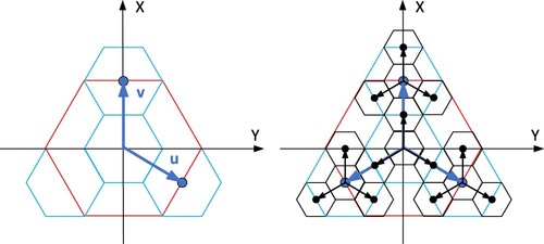
The vector model of the hexagonal lattice is constructed by describing the hexagonal lattice with vectors. In every resolution of hexagonal grids, each hexagonal cell can be represented by the combination of $\mathit{u}$ and $\mathit{v}$. Let $P_n$ denote the set of all lattices that are partitioned in the $n\mathrm{t}\mathrm{h}$ resolution of hexagonal grids; it can be expressed as follows: (1) $\begin{array}{c}{P}_n=P_{n-1}+D,P_n=P_0+\sum _{i=1}^n{\displaystyle \frac{1}{2^{i-1}}D\left(n\ge 1\right)}\end{array}$(1) where $\mathit{D}=\left\{0,\mathit{u},\mathit{v},-\mathit{u}-\mathit{v}\right\}$ indicates the direction of the partition and $P_0$ represents the lattice of the first level.

For $n\ge 1$, let ${\mathit{u}}_{\mathit{n}}={\displaystyle \frac{1}{2^{n-1}}\mathit{u}}$, ${\mathit{v}}_{\mathit{n}}={\displaystyle \frac{1}{2^{n-1}}\mathit{v}}$ and $L_n$ be the linear combination of ${\mathit{u}}_{\mathit{n}}$ and ${\mathit{v}}_{\mathit{n}}$. It is easy to determine that $L_n$ represents all lattices in the $n\mathrm{t}\mathrm{h}$ level vector space. (2) $\begin{array}{c}{L}_n=n_1{\mathit{u}}_{\mathit{n}}+n_2{\mathit{v}}_{\mathit{n}};n_1,n_2\in Z\end{array}$(2) Properties of ${\mathit{P}}_{\mathit{n}}$. The following properties are easily obtained from the definitions of $P_n$ and $L_n$ and are fundamental theorems for the aperture 4 hexagonal DGGS:

1. $forn\ge 1,P_n\subset L_n$

2.	$P_n$ are nested: $P_0\subset P_1\subset P_2\subset \cdots$

3. The number of lattice points in $P_n$ is $4^n$

4.	For any $n\ge 0$ and $P_i\in P_n$, there exists a unique $d_i\in \left\{0,{\displaystyle \frac{1}{2^i}\mathit{u},{\displaystyle \frac{1}{2^i}\mathit{v},{\displaystyle \frac{1}{2^i}\left(-\mathit{u}-\mathit{v}\right)}}}\right\}$, (3) $\begin{array}{c}{P}_i=\sum _{i=1}^n{d}_i\end{array}$(3)

The mathematical proof of Property 4 is presented in Appendix (1). Property 4 can be used as follows to assign each cell in $P_n$ a label (address) that consists of a string of n digits from the set {0, 1, 2, 3, 4}. Equation (4) is referred to as the standard form for $P_i$ in $P_n$. Let $a_i\in \left\{0,1,2,3,4\right\}$. The string $\alpha =a_1{a}_2....a_n$ of integers in the standard form is referred to as the label of $P_i$ in $P_n$, it is a one-to-one correspondence between the label and the hexagonal cell. Figure 6 shows the labels of $P_1$ and $P_3$.

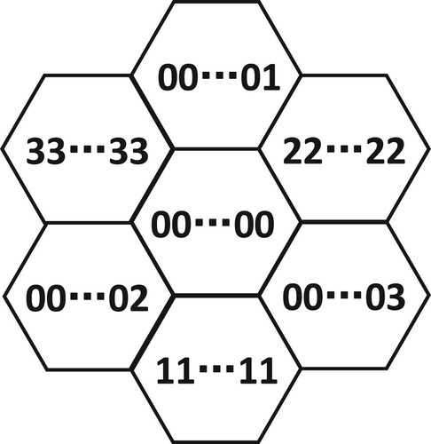
As shown in Figure 6, quadtree encoding will cause encoding gaps and uniqueness problems, and cannot cover the entire spherical surface, so it needs to be adjusted. For the code in the lower right corner, the excess hexagonal grids can be expressed as: (4) $\begin{array}{c}R{L}_n=\left(2^{n-1}+n_1\right){\mathit{u}}_{\mathit{n}}+n_2{\mathit{v}}_{\mathit{n}};2n_1-n_2>2,n_1,n_2\in Z\end{array}$(4) The set of hexagonal grids in the upper left corner can be expressed as: (5) $\begin{array}{c}R{L}_n^{\ast }=(2^{n-1}+n_1){\mathit{u}}_{\mathit{n}}^{\ast }+n_2{\mathit{v}}_{\mathit{n}}^{\ast };2n_1-n_2>2,n_1,n_2\in Z\end{array}$(5) $\mathit{u}〈=〉{\mathit{u}}_{\mathit{n}}^{\ast }$, $\mathit{v}〈=〉{\mathit{v}}_{\mathit{n}}^{\ast }$, and then $R{L}_n〈=〉R{L}_n^{\ast }$. 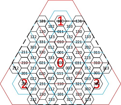The mathematical proof is provided in Appendy (2). The part of the grid that exceeds the lower right corner exactly corresponds to the part that is vacant in the upper left corner. Similarly, the part of the grid that exceeds the upper and lower left corners can also correspond to the empty part in the lower and upper right corners, respectively. Therefore, we can construct an optimized hexagonal quadtree structure by means of translation transformation, as shown in Figure 7.

Figure 6. The labels of $P_1$ and $P_3$

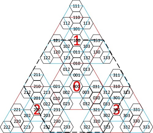
Figure 7. Optimized Hexagonal QuadTree Structure

3. Operations of the OHQS DGGS

3.1 Rule of code addition

3.1.1 Addition based on induction

A vector represents the center point of the hexagonal cell, and the corresponding code is constructed. The code records the distance and orientation of the hexagonal lattice relative to the origin lattice. Similar to vector addition, the parallelogram rule can be used to define the code addition operation. According to induction and verification, the coded addition satisfies the properties of the Abelian group.

The rules of code addition in the current study are similar to the addition rules for integers (Vince and Zheng 2009; Tong et al. 2013; Wang et al. 2019). The code of the $n\mathrm{t}\mathrm{h}$ resolution $\alpha =a_1{a}_2....a_n$ and $\text{β}=b_1{b}_2....b_n$, The calculation method of code addition is similar to that of decimal addition. The method starts from the last symbol on the right and calculates bit by bit to the first symbol on the left. The code addition operation can be decomposed into the sum of the corresponding codes for different additions. (6) $\begin{array}{c}\alpha \oplus \text{β}=a_1{a}_2..a_n\oplus b_1{b}_2..b_n=\left(a_1\oplus b_1\right)\left(a_2\oplus b_2\right)..\left(a_n\oplus b_n\right)\end{array}$(6) The same process applies to the decimal addition operation rule. For all the code elements to be added and the calculation result code element of the current bit, a carry code element will be generated on the left side. The specific operation rules are expressed as follows: (7) $a_n\oplus b_n=\{\begin{array}{c}{a}_{n}0\left(a_n=b_n\right)\\ a_n\left(a_n\ne 0,b_n=0\right)\\ \underset{n}{c\dots \dots c}(a_n\ne b_n,a_n\ne 0,b_n\ne 0,c=\overline{\left\{0,a_n,b_n\right\}}\end{array}$(7) In the calculation process, when $a_n\ne b_n$, a large number of carry symbols will be generated on the addition bit, and the number of addition operations on each resolution exponentially increases. To improve the calculation efficiency, the number of addition operations must be reduced. Analyzing the rule of addition, the optimization methods can be described as follows:

1. 0 can be ignored as a calculation code element. When the code elements are identical, only one carry code element is generated so that the same code element can be calculated first. Only three symbols $\left\{1,2,3\right\}$ remain, they participate in the addition algorithm.

2. It is unnecessary to store every carry symbol but only count the number of symbols that appear in addition, which can save considerable calculation memory. $c=\overline{\left\{0,a_n,b_n\right\}}$ can be realized by the binary XOR ($\wedge$) operation: $c=a_n\wedge b_n$.

In the calculation process, when $a_n\ne b_n$, numerous carry symbols are generated. By adopting the method of counting the number of occurrences of symbols and by preferentially calculating the same symbols, the number of symbol calculations can be reduced (Wang et al. 2018; Wang et al. 2019). Through the above steps, the computational efficiency of code addition can be significantly improved, and Algorithm 1 shows the process of code addition for the OHQS.

Algorithm 1: SUM($a_1{a}_2....a_n$, $b_1{b}_2....b_n$)

Input: Two labels $a_1{a}_2....a_n$ and $b_1{b}_2....b_n$

Output: If it exists, SUM = $a_1{a}_2....a_n\oplus b_1{b}_2....b_n$. Otherwise, SUM = overflow.

Step 1. Initialize two-dimensional array A[n][4] to record the number of every digit that participates in the calculation in digit position $i$ (position of $a_i$ and $b_i$). Let A[n][4] record the digits of labels $\alpha$ and $\text{β}$ first.

Step 2. For $i=nto2$ (right to left), do. (8) $\begin{array}{c}A\left[i+1\right]\left[j\right]={\displaystyle \frac{A\left[i\right]\left[j\right]}{2},A\left[i\right]\left[j\right]=A\left[i\right]\left[j\right]\text{\%}2,j\in \left\{1,2,3\right\}}\end{array}$(8) The number of remaining digits is three at most. The remaining digits can be input in the calculation by Equation. (8).

Step3. $A\left[1\right]\left[j\right]=A\left[1\right]\left[j\right]\text{\%}2,j\in \left\{1,2,3\right\}$, and then the first number of results can be calculated.

Unlike the HLQT, the first code is not defined in this paper. The HLQT code consists of the first symbol and subsequent digits. The set of first symbols in the HLQT is $E=\{0,1,2,3,4,5,6,10,20,30,40,50,60,100,200,300,400,500,600,106,601,201$, $102,302,203,403,304,504,405,605,506,1000,2000,3000,4000,5000,6000\}$ (Wang et al. 2019). Since there is no addition table built for some of these symbols, the HLQT builds complex rules to avoid its addition. Notably, the binary algorithm is utilized to realize the addition. For example, for $c=\overline{\left\{0,a_n,b_n\right\}}$, the addition can be realized by binary operation $c=a_n\wedge b_n$. Compared with the HLQT, the efficiency of the addition operation of the OHQS was greatly improved.

3.1.2 Addition based on ijk coordinate

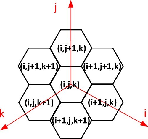
Although the efficiency has been improved, Algorithm 1 still has difficulty meeting the needs of practical applications. We attempt to implement the addition by transformation between OHQS codes and $ijk$ coordinates. The $ijk$ coordinate can be utilized to represent the relative position of the hexagonal grid in the space, as shown in Figure 8. The coordinate axis divides the space into 3 quadrants, and the coordinates in each quadrant are represented by two adjacent coordinate axes. The $ijk$ coordinates are always positive, which is easy to calculate. In this paper, the OHQS code is converted to $ijk$ coordinates, and the addition operation is performed in three dimensions in the $ijk$ coordinate system. The addition result is converted to a code.

Figure 8. $ijk$ coordinate system

We need to realize the transformation between OHQS codes and the $ijk$ coordinates. The directions of the three coordinate axes in the $ijk$ coordinate system are equivalent to $\mathit{u}$, $\mathit{v}$, and $-\mathit{u}-\mathit{v}$ in the vector model of the hexagonal lattice. Formulas (1) and (2) show that the units of the $i$, $j$, and $k$ coordinate axes of the nth resolution are ${\displaystyle \frac{1}{2^{n-1}}\left|\mathit{u}\right|}$, ${\displaystyle \frac{1}{2^{n-1}}\left|\mathit{v}\right|}$ and ${\displaystyle \frac{1}{2^{n-1}}\left|-\mathit{u}-\mathit{v}\right|}$. Each hexagonal grid can be expressed as $\left[r,\left(i,j,k\right)\right]$ in the ijk coordinate system, where $r$ represents the resolution of the hexagonal grid. For each digit $a_r$ in the OHQS code, from Formula (3), we know that $a_r\equiv d_r\in \left\{0,{\displaystyle \frac{1}{2^{r-1}}\mathit{u},{\displaystyle \frac{1}{2^{r-1}}\mathit{v},{\displaystyle \frac{1}{2^{r-1}}\left(-\mathit{u}-\mathit{v}\right)}}}\right\}$. We can obtain the correspondence between digits and $ijk$ coordinates. Next, the transformation relationship between the OHQS code $\alpha \left(a_1{a}_2....a_n\right)$ and the $ijk$ coordinate can be obtained, and Algorithm 2 for converting the code to coordinates and Algorithm 3 for converting the coordinates to code can be constructed.

In the calculation of converting the encoding into $ijk$ coordinates, first, we separately calculate the $ijk$ values of each resolution in the order of encoding, and accumulate the results to obtain $\left(i,j,k\right)$. Second, because the value of three coordinate axes will be generated in the calculation, it needs to be converted to $\left[n,\left(i,j,k\right)\right]$, which is represented by two coordinate axes. Last, since the translation transformation of the encoding is performed by using Formulas (4) and (5), the translation transformation of the $ijk$ coordinates also needs to be performed in the calculation. The mathematical proof of Formula (9) is provided Appendix (3).

Algorithm 2:

CodeToijk$(a_1{a}_2....a_n)$

Input: code $a_1{a}_2....a_n$

Output: $ijk\left[n,\left(i,j,k\right)\right]$

Step 1. Calculate $\left(i,j,k\right)$. (9) $\begin{array}{c}\left(\begin{array}{c}\begin{array}{c}i\\ j\end{array}\\ k\end{array}\right)=\sum _{p=0}^{n-1}\left\{{\left(\begin{array}{cc}\begin{array}{c}\begin{array}{cc}2& 0\\ 0& 2\end{array}\\ \begin{array}{cc}0& 0\end{array}\end{array}& \begin{array}{c}0\\ 0\\ 2\end{array}\end{array}\right)}^p\cdot \phi \left(a_{p+1}\right)\right\}\end{array}$(9) where $n$ represents the length of the code and $\phi \left(a_{p+1}\right)$ is given in Table 1.

Table 1. $\phi$ values associated with different digits

	0	1	2	3
$\phi$	$\left(\begin{array}{c}\begin{array}{c}0\\ 0\end{array}\\ 0\end{array}\right)$	$\left(\begin{array}{c}\begin{array}{c}0\\ 1\end{array}\\ 0\end{array}\right)$	$\left(\begin{array}{c}\begin{array}{c}0\\ 0\end{array}\\ 1\end{array}\right)$	$\left(\begin{array}{c}\begin{array}{c}1\\ 0\end{array}\\ 0\end{array}\right)$

Step 2. Convert $\left(i,j,k\right)$ to [n, (i,j,k)], which is represented by two coordinate axes.

Let $m=min\left(i,j,k\right);i=i-m;j=j-m;k=k-m.$

Step 3. Obtain the translation transformation of the $ijk$ coordinates. $\begin{array}{rl}ifi& =0\mathrm{\&}\mathrm{\&}2\times j-k>2^n,theni=2^n-j,k=k+i,j=0;\\ & elseifi=0\mathrm{\&}\mathrm{\&}2\times k-j\\ & >2^n,theni=2^n-k,j=j+i,k=0;elseifj=0\mathrm{\&}\mathrm{\&}2\times i-k\\ & >2^n,thenj=2^n-i,k=k+j,i=0;esleifj=0\mathrm{\&}\mathrm{\&}2\times k-i\\ & >2^n,thenj=2^n-k,i=i+j,k=0;elseifk=0\mathrm{\&}\mathrm{\&}2\times i-j\\ & >2^n,thenk=2^n-i,j=j+k,i=0;elseifk=0\mathrm{\&}\mathrm{\&}2\times j-i\\ & >2^n,thenk=2^n-j,i=i+k,j=0.\end{array}$In the calculation of converting $\left[n,\left(i,j,k\right)\right]$ to code, first, the offset vector of each resolution of the DGGS is sequentially calculated from the 1st resolution to the nth resolution. The offset vector refers to the offset value of each layer symbol relative to the previous layer in the vector mathematical model. The offset vector refers to the offset value of the digits of each resolution relative to the digits of the previous resolution in the vector model. Second, according to the correspondence between the offset vector and the digit in Table 2, the value of the digit of each resolution is determined, and last all the digits are combined to form the OHQS code $a_1{a}_2....a_n$.

Table 2. Relationship between offset vector and digit

offset vector	$\left(Vi,Vj,Vk\right)$	digit $a_r$
$\left(0,0,0\right)$	$\left(0,0,0\right)$	0
$\{\begin{array}{c}\left(0,{\displaystyle \frac{1}{2^{r-1}}v,0}\right)\\ \left({\displaystyle \frac{1}{2^{r-1}}u,0,{\displaystyle \frac{1}{2^{r-1}}\left(-\mathit{u}-\mathit{v}\right)}}\right)\end{array}$	$\{\begin{array}{c}\left(0,1,0\right)\\ \left(1,0,1\right)\end{array}$	1
$\{\begin{array}{c}\left(0,0,{\displaystyle \frac{1}{2^{r-1}}\left(-\mathit{u}-\mathit{v}\right)}\right)\\ \left({\displaystyle \frac{1}{2^{r-1}}u,{\displaystyle \frac{1}{2^{r-1}}v,0}}\right)\end{array}$	$\{\begin{array}{c}\left(0,0,1\right)\\ \left(1,1,0\right)\end{array}$	2
$\{\begin{array}{c}\left({\displaystyle \frac{1}{2^{r-1}}u,0,0}\right)\\ \left(0,{\displaystyle \frac{1}{2^{r-1}}v,{\displaystyle \frac{1}{2^{r-1}}\left(-\mathit{u}-\mathit{v}\right)}}\right)\end{array}$	$\{\begin{array}{c}\left(1,0,0\right)\\ \left(0,1,1\right)\end{array}$	3

Algorithm 3:

ijkToCode($\left[n,\left(i,j,k\right)\right]$)

Input: $ijk\left[n,\left(i,j,k\right)\right]$, the offset vector $\left(Vi,Vj,Vk\right)$

Output: code $a_1{a}_2....a_n$ $forr=1tondo$Step 1. Calculate the offset vector. $Vi=i\mathrm{\&}1;Vj=j\mathrm{\&}1;Vk=k\mathrm{\&}1;i=i>>1;j=j>>1;k=k>>1;$Step 2. Determine the r-th digit in the code according to the offset vector. $if\left(Vi=0\mathrm{\&}\mathrm{\&}Vj=1\mathrm{\&}\mathrm{\&}Vk=0\right)or\left(Vi=1\mathrm{\&}\mathrm{\&}Vj=0\mathrm{\&}\mathrm{\&}Vk=1\right),then$ $a_r=1;elseif\left(Vi=0\mathrm{\&}\mathrm{\&}Vj=0\mathrm{\&}\mathrm{\&}Vk=1\right)or(Vi=1\mathrm{\&}\mathrm{\&}Vj=1\mathrm{\&}\mathrm{\&}Vk$ $=0),then{a}_r=2;elseif(Vi=1\mathrm{\&}\mathrm{\&}Vj=0\mathrm{\&}\mathrm{\&}Vk=0\left)or\right(Vi=0\mathrm{\&}\mathrm{\&}Vj$ $=1\mathrm{\&}\mathrm{\&}Vk=1),then{a}_r=3;else{a}_r=0.$The addition algorithm based on $ijk$ coordinate transformation utilizes Algorithm 2 and Algorithm 3. For the two codes $a_1{a}_2....a_n$ and $b_1{b}_2....b_n$ to be calculated, first, the two codes are converted to $ijk$ coordinates $\left[n,i_1,j_1,k_1\right]$ and $\left[n,i_2,j_2,k_2\right]$. Second, the addition operation is performed in three dimensions in the $ijk$ coordinate system, and last the result of the operation is converted to the OHQS code.

Algorithm 4:

$SU{M}^{\ast }$($a_1{a}_2....a_n$, $b_1{b}_2....b_n$)

Input: code $a_1{a}_2....a_n$ and $b_1{b}_2....b_n$

Output: if the result exists, $SU{M}^{\ast }$ = $a_1{a}_2....a_n\oplus b_1{b}_2....b_n$. else, $SU{M}^{\ast }$ = overflow.

Step 1. $ij{k}_1\left[n,i_1,j_1,k_1\right]=CodeToijk\left(a_1{a}_2....a_n\right)$, $ij{k}_2\left[n,i_2,j_2,k_2\right]=CodeToijk\left(b_1{b}_2....b_n\right)$.

Step 2. $ij{k}_3\left[n,i_3,j_3,k_3\right]=ij{k}_1\left[n,i_1,j_1,k_1\right]+ij{k}_2\left[n,i_2,j_2,k_2\right]$.

m = Min$i_3,j_3,k_3$, $ij{k}_3$ = $ij{k}_3\left[n,i_3,j_3,k_3\right]-ij{k}_m\left[n,i_m,j_m,k_m\right]$.

Step3. $SU{M}^{\ast }=\mathrm{i}\mathrm{j}\mathrm{k}\mathrm{T}\mathrm{o}\mathrm{C}\mathrm{o}\mathrm{d}\mathrm{e}\left(\left[n,i_3,j_3,k_3\right]\right)$

3.2 Rule of adjacent grid retrieval

Based on the additional rules of the OHQS code, the adjacent grid retrieval operation of the hexagonal cell can be constructed. The six adjacent codes of the grid code can be obtained by adding adjacent codes of the center code on the OHQS. As shown in Figure 9, the six adjacent codes of the center code are $\underset{n-1}{\underset{}{00\dots 0}}1$, $\underset{n-1}{\underset{}{00\dots 0}}2$, $\underset{n-1}{\underset{}{00\dots 0}}3$, $\underset{n}{\underset{}{22\dots 22}}$, $d_5=\underset{n}{\underset{}{11\dots 11}}$, and $d_6=\underset{n}{\underset{}{33\dots 33}}$.

Figure 9. Six adjacent cells in the center of the OHQS code

The adjacent grid retrieval operation based on the ijk coordinate transformation is relatively simple. First, we use Algorithm 2 to convert the OHQS code to $\left(i,j,k\right)$ coordinates. Second, we calculate the $ijk$ coordinates of the six adjacent grids $\left(i,j+1,k\right)$, $\left(i+1,j+1,k\right)$, $\left(i+1,j,k\right)$, $\left(i+1,j,k+1\right)$, $\left(i,j,k+1\right)$, and $\left(i,j+1,k+1\right)$, as shown in Figure 10. Last we use Algorithm 3 to convert the six $ijk$ coordinates to codes.

Figure 10. Six adjacent grids in the center of the OHQS code

3.3. Transformation between OHQS codes and geographic coordinate system

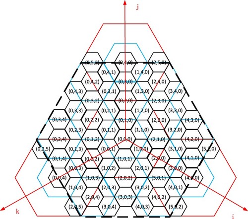
Although there are various storage formats, most existing spatial data are usually represented by geographic coordinates or projected coordinates. To facilitate the organization and expression of spatial data in the DGGS, it is necessary to construct the transformation between geographic coordinates and global discrete grid codes. Based on the characteristics of the OHQS encoding scheme, this paper designs and implements an efficient transformation algorithm between codes and geographic coordinates. The algorithm involves six coordinate systems: (1) OHQS codes that can be regarded as a one-dimensional coordinate system, (2) $ij$ coordinate system, (3) $ijk$ coordinate system, (4) $IJK$ coordinate system, (5) two-dimensional cartesian coordinate system on the triangular surface of an icosahedron, and (6) geographic coordinate system. 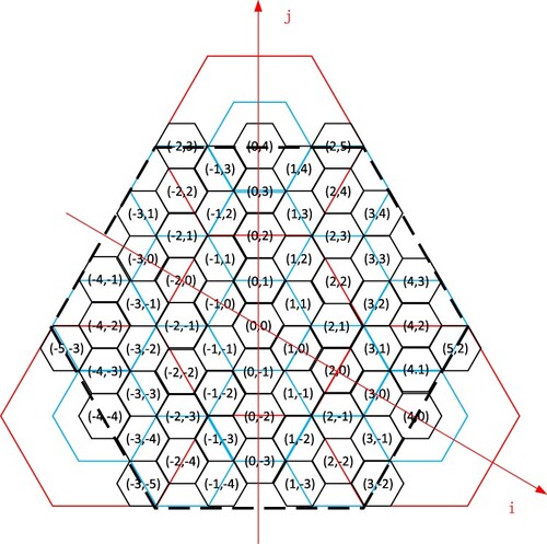Compared with the $ijk$ coordinate system, the $ij$ coordinate system has one fewer coordinate axis. The origin point is located at the center of the origin hexagon, and the coordinate axes are aligned with the two sides of the origin hexagon. Each hexagonal grid can be uniquely determined by $\left(i,j\right)$ coordinates which are integer values. Figure 11 illustrates the assignment of the coordinate address. The $IJK$ coordinate system is different from the $ijk$ coordinate system. Figure 12 show the IJK coordinate system. The coordinate value in the IJK coordinate system is the vertical projection of the lattice point on the coordinate axis, and can be negative. The units of the $I$, $J$, and $K$ coordinate axes of the nth resolution are ${\displaystyle \frac{1}{2^n}\left|\mathit{u}\right|}$, ${\displaystyle \frac{1}{2^n}\left|\mathit{v}\right|}$ and ${\displaystyle \frac{1}{2^n}\left|-\mathit{u}-\mathit{v}\right|}$. The $IJK$ coordinates of each lattice point satisfy the following formula: (10) $\begin{array}{c}I+J+K=0\end{array}$(10) (11) $\begin{array}{c}\left(I+J\times 2\right)\text{\%}3=0\end{array}$(11)

Figure 11. $ij$ coordinate system

3.3.1 From codes to the geographic coordinate system

According to the grid code, we can calculate the geographic coordinates of the center point and six vertices of the grid where the code is located. Unlike the complex expansion of the HLQT, we directly implement the transformation from code to geographic coordinates through the $ij$ coordinate system. This transformation algorithm can calculate the geographic coordinates of the center point. The other six vertices are identical. First, the OHQS codes are converted to the $\left(i,j\right)$ coordinates, Second the $\left(x,y\right)$ coordinates of the Cartesian coordinate system are obtained by the $\left(i,j\right)$ coordinates. Last, the geographic coordinates $\left(B,L\right)$ can be calculated by the Snyder equal-area projection. Figure 13 and Algorithm 5 show the transformation process from codes to geographic coordinates.

Figure 12. $IJK$ coordinate system

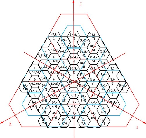
Figure 13. Transformation process from codes to geographic coordinates: (a) $ij$ coordinate system, (b) Cartesian coordinate system, and (c) geographic coordinate system

Algorithm 5:

CodeToCoordinate(code)

Input: One label $a_1{a}_2....a_n$

Output: Geographic coordinate $\left(B,L\right)$ of the center point of the hexagonal cell

Step 1. Calculate $\left(i,j\right)$. (12) $\begin{array}{c}\left(\begin{array}{c}i\\ j\end{array}\right)=\sum _{k=0}^{n-1}\left\{{\left(\begin{array}{cc}2& 0\\ 0& 2\end{array}\right)}^k.\omega \left(a_{k+1}\right)\right\}\end{array}$(12) where $n$ denotes the length of the label and the results of $\omega \left(a_{\mathrm{k}+1}\right)$ are given in Table 3.

Step 2. if $2\times j-i>2^n:j=j-2^n;elseif-i-j>2^n:i=i+2^n,j=j+2^n;elseif2\times i-j>2^n:i=i-2^n.$

Step 3. Calculate $\left(x,y\right)$. (13) $\begin{array}{c}\left(\begin{array}{c}x\\ y\end{array}\right)=\left(\begin{array}{cc}{\left({\displaystyle \frac{1}{2}}\right)}^{n+1}\cdot L& 0\\ -{\displaystyle \frac{\sqrt{3}}{3}\cdot {\left({\displaystyle \frac{1}{2}}\right)}^{n+1}\cdot L}& {\displaystyle \frac{\sqrt{3}}{3}\cdot {\left({\displaystyle \frac{1}{2}}\right)}^n\cdot L}\end{array}\right)\cdot \left(\begin{array}{c}i\\ j\end{array}\right)\end{array}$(13) where $L$ denotes the length of the triangular surface of the icosahedron.

Step 4. $\left(B,L\right)$ can be calculated by the Snyder equal-area projection.

3.3.2 From the geographic coordinate system to codes

If we obtain the geographic coordinate $\left(B,L\right)$ of a point, the OHQS code at which the point is located can be obtained by a transformation algorithm. The HLQT uses the parallelogram rule to project the coordinates to two specific coordinate axes, calculates the corresponding component codes on the two axes, and then calculates the final code through component code addition. We realize the transformation from geographic coordinates to code through the mutual conversion of the $IJK$ coordinate system, $ij$ coordinate system and $ijk$ coordinate system. First, the $\left(B,L\right)$ coordinate is converted to the $\left(x,y\right)$ coordinate by the inverse Snyder projection. Because there are errors in the direct process of converting the $\left(x,y\right)$ coordinate to the $\left(i,j\right)$ coordinate, second we introduce the $IJK$ coordinate system to obtain the $\left(i,j\right)$ coordinate. 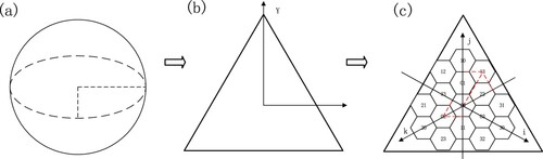Last, we convert the $\left(i,j\right)$ coordinate to the $\left(i,j,k\right)$ coordinate, and the code $\alpha$ can be calculated by the coordinate transformation of Algorithm 3. Figure 14 and Algorithm 6 show the transformation process from geographic coordinates to codes.

Figure 14. Transformation process from geographic coordinates to codes: (a) geographic coordinate system, (b) Cartesian coordinate system, (c) $ijk$ coordinate system

Algorithm 6: CoordinateToCode(B, L)

Input: geographic coordinate $\left(B,L\right)$ of one point.

Output: Code $\alpha$ of the hexagonal cell at resolution $n$, which contains the point.

Step 1. The geographic coordinate $\left(B,L\right)$ is transformed to the $\left(x,y\right)$ coordinate.

Step 2. Calculate the $IJK$ coordinate as follows: (14) $\begin{array}{c}\left(\begin{array}{c}I\\ J\\ K\end{array}\right)=\left(\begin{array}{cc}{\displaystyle \frac{\sqrt{3}}{2}}& -{\displaystyle \frac{1}{2}}\\ 0& 1\\ -{\displaystyle \frac{\sqrt{3}}{2}}& -{\displaystyle \frac{1}{2}}\end{array}\right)\cdot \left(\begin{array}{c}x\\ y\end{array}\right)\end{array}$(14) Step 3. Calculate the $IJK$ coordinate of the center point of possibly relevant hexagonal cells. A total of eight coordinates are stored in the array $V\left[8\right]\left[3\right]$. (15) $V\left[8\right]\left[3\right]=\left[\begin{array}{c}\begin{array}{ccc}I/m& J/m& K/m\\ I/m& J/m& K/m\\ I/m& J/m& K/m\end{array}\\ \begin{array}{ccc}I/m& J/m& K/m\\ I/m& J/m& K/m\\ I/m& J/m& K/m\end{array}\\ \begin{array}{ccc}I/m& J/m& K/m\\ I/m& J/m& K/m\end{array}\end{array}\right],m={\left({\displaystyle \frac{1}{2}}\right)}^{n+1}\cdot L\cdot {\displaystyle \frac{\sqrt{3}}{3}}$(15) where $L$ denotes the length of the triangular surface of an icosahedron, and $m$ indicates the side length of the hexagon in resolution $n$.

Step 4. For $i=0to8$, if $V\left[i\right]\left[0\right]+V\left[i\right]\left[1\right]+V\left[i\right]\left[2\right]==0\mathrm{\&}\mathrm{\&}\left(V\left[i\right]\left[0\right]+V\left[i\right]\left[1\right]\cdot 2\right)\text{\%}3==0$, then. (16) $\begin{array}{c}\left(\begin{array}{c}i\\ j\end{array}\right)=\left(\begin{array}{cc}{\displaystyle \frac{2}{3}}& {\displaystyle \frac{1}{3}}\\ {\displaystyle \frac{1}{3}}& {\displaystyle \frac{2}{3}}\end{array}\right)\cdot \left(\begin{array}{c}V\left[i\right]\left[0\right]\\ V\left[i\right]\left[1\right]\end{array}\right)\end{array}$(16) Step 5. Convert the $\left(i,j\right)$ coordinate to the $\left(i,j,k\right)$ coordinate and then use Algorithm 3 ijkToCode($\left[n,\left(i,j,k\right)\right]$) to calculate the OHQS code.

3.4. Spatial data modeling on a discrete global grid system

The organization and expression of spatial data is an essential key issue in processing and application, and it must be carried out in a specific digital space. Plane-based digital space and data expression methods have been significantly restricted in processing global or large-scale massive spatial data. It is urgent to establish an effective data expression method in a suitable digital space with characteristics such as uniformity and multiple scales. The hexagonal global discrete grid system is just an alternative form of spherical digital space. As previously mentioned, the OHQS code of the global discrete grid constructed in this paper implicitly expresses the spatial position. Additionally, the OHQS code carries information such as the scale and accuracy of the data and has the characteristics of multiresolution and the potential ability to process multiscale data. This part mainly addresses the construction of traditional spatial data (vector data and raster data) in the global discrete grid system.

Both raster data and discrete global grids are discretizations of space. Rectangular grids are employed in raster data to partition space on a plane, while regular polygons are utilized in discrete global grids to partition spherical space. It is necessary to establish a data conversion model from raster data to a discrete global grid. The first step is to determine the level of the hexagonal grid that corresponds to the raster data according to the resolution of the raster data and the area of the hexagon. Table 4 shows the area of the hexagonal grid on different DGGS levels. Let initial area $a=17,002,187.39080$. The best level to raster data conversation is: (17) $\begin{array}{c}n={\displaystyle \frac{{\log }_{4}a}{RX\times RY}+1}\end{array}$(17) where $n$ denotes the best level for data conversation, and $RX$ and $RY$ denote the resolution of the raster data on the $x$ axis and $y$ axis, respectively.

Table 3. $\omega$ corresponds to different code cells

Code cells	0	1	2	3
$\omega$	$\left(\begin{array}{c}0\\ 0\end{array}\right)$	$\left(\begin{array}{c}0\\ 1\end{array}\right)$	$\left(\begin{array}{c}-1\\ -1\end{array}\right)$	$\left(\begin{array}{c}1\\ 0\end{array}\right)$

Table 4. ISEA4H attribute at different resolutions

Resolutions	Number of cell	Hex area$\left(k{m}^2\right)$	Pen area$\left(k{m}^2\right)$
1	32	17,002,187.39080	14,168,489.49230
2	122	4,250,546.84770	3,542,122.37308
3	482	1,062,636.71193	885,553.59327
4	1,922	265,659.17798	221,382.64832
5	7,682	66,414.79448	55,345.66208
6	30,722	16,603.69862	13,836.41552

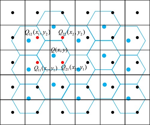
There are three methods to resample raster values to DGGS grids: nearest-neighbor interpolation, bilinear interpolation, and bicubic interpolation. Compared with other methods, bilinear interpolation can guarantee higher interpolation accuracy and calculation efficiency (Ma et al. 2021). Figure 15 shows a schematic of the interpolation operation between pixels and hexagons.

Figure 15. Schematic of the interpolation operation

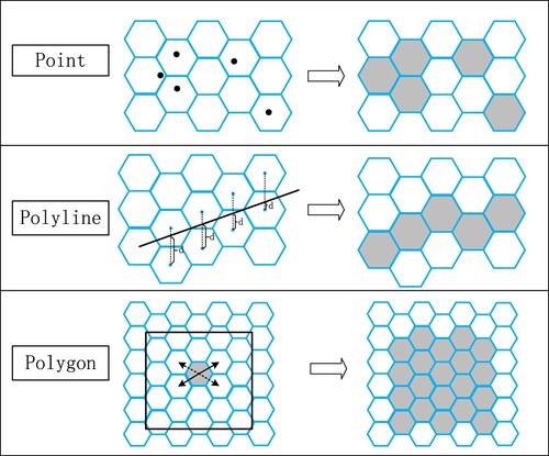
For vector data, the best DGGS resolution to express the vector data can be selected according to the positional accuracy of the vector data. To sample the vector data into discrete global grid systems, as shown in Figure 16, the Bresenham algorithm (Bresenham 1977) is used to implement a polyline vector data conversation. The scan line seed fill algorithm is employed to implement vector data conversation of a polygon. The value of the attribute of vector data is assigned to DGGS grids.

Figure 16. Data conversation diagram of vector data

4. Results

Presently, the hexagonal DGGS encoding schemes that are most commonly utilized in research and applications are PYXIS, HQBS, and HLQT (Vince and Zheng 2009; Peterson 2011; Tong et al. 2013; Wang et al. 2018; Wang et al. 2019; Wang et al. 2021). Previous studies have demonstrated that the code addition efficiency of the HLQT is superior to that of the HQBS and PYXIS, and that the transformation efficiency of the HLQT is superior to that of HQBS. This paper compares the operation efficiency of the OHQS with that of the HLQT (Tong et al. 2013; Wang et al. 2018; Wang et al. 2021).

To verify the efficiency and advantages of the above algorithms, comparison experiments are designed to test the efficiency of the addition operation, adjacent cell retrieval, and transformation between the OHQS and the HLQT. The experiments are conducted on a desktop computer(operating system: Windows 7, hardware configuration: Intel Core i5-6500 [email protected] GHZ and 16.0 GB RAM.

4.1 Results and comparison of code addition and adjacent cell retrieval

4.1.1 Comparison of the lengths of different encodings

We compared the encoding lengths of the HLQT and OHQS at the same position. The comparison of different encoding results is shown in Table 5. $I{\alpha }_n$ and $J{\alpha }_n$ are OHQS codes, and $I{\text{β}}_n$ and $J{\text{β}}_n$ are HLQT codes. We compress the OHQS code to obtain the decimal code. By comparison, it can be determined that the OHQS encoding is relatively simpler, that there is no need to use commas to separate the first symbol, and that the OHQS encoding can also be converted to decimal code to further compress the encoding.

4.1.2 Comparison of the efficiency of code addition and adjacent cell retrieval

The efficiency of addition and adjacent cell retrieval in the DGGS is associated with the encoding scheme and calculation algorithm, encoding resolution, and number of code operations. We test three operations of the HLQT and OHQS based on induction and the OHQS based on the $ijk$ coordinate. In the addition algorithm test, 100000 pairs of codes are randomly selected from each resolution to realize the calculation. In the adjacent cell retrieval operation, 100000 codes are randomly chosen to obtain the six adjacent codes. The calculation efficiency from resolutions 5–12 was tested ten times, and the unit is $ms$. The efficiency of addition and adjacent cell retrieval results between OHQS and HLQT are shown in Figure 17 and Table 6.

Figure 17. Comparison of the efficiency of addition and adjacent cell retrieval between the OHQS and the HLQT

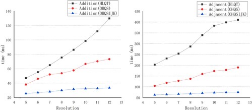
Table 5. Comparison of different encoding results

Res	code$I{\alpha }_n$	Decimal code	code $I{\text{β}}_n$	code $J{\alpha }_n$	decimal code	code $J{\text{β}}_n$
1	3	3	none	1	1	none
2	32	14	60	13	7	506
3	320	56	60,0	131	29	506,1
4	3201	225	60,01	1310	116	506,10
5	32012	902	60,012	13101	465	506,101
6	320121	3609	60,0121	131012	1862	506,1012

Table 6. Computation time for experiments (ms)

Res	Addition			Adjacent grid retrieval
	HLQT	OHQS	$ijk$	HLQT	OHQS	$ijk$
5	46.9	38	25.5	202.7	104.4	62.9
6	55.2	45.9	26.8	231.4	118.3	65
7	64.9	51.9	28	253.5	127.9	67
8	75.5	53.6	29.9	286.7	137	68.5
9	86.4	57.7	31.7	339.3	159.3	71.3
10	98.6	66.6	32.3	383.1	173.3	73.2
11	111.9	70.3	32.6	398.4	178.4	74.8
12	129.9	73.2	33.4	410.2	189.8	75.3

In the addition operation of the DGGS, the efficiency of the OHQS based on induction is higher than that of the HLQT, and the efficiency of the OHQS based on $ijk$ transformation is much higher than that of both. As the resolution of the DGGS increases, the efficiency of the OHQS based on $ijk$ transformation is affected the least, followed by that of the OHQS based on induction, while the impact on the HLQT rapidly increases. In the adjacent grid retrieval operation, the efficiency of OHQS based on $ijk$ transformation is twice that of the OHQS based on induction and four times that of the HLQT. With an increase in the resolution of the DGGS, the efficiency of adjacent grid retrieval of the OHQS based on $ijk$ transformation suffers the least, while the HLQT suffers the most. The adjacent grid retrieval operation is built on six code additions. The adjacent operation time of the HLQT is 4 times that of the addition operation, and the adjacent operation time of the OHQS based on $ijk$ transformation and induction is 2.5 times that of the addition operation. The results are analyzed as follows.

1. The HLQT constructs addition tables and addition rules by means of induction, which is not only cumbersome but also computationally complex. Although it is reduced from $O\left(2^N\right)$ to $O\left(N^2\right)$ through a series of methods, the operation efficiency is still slow. In this paper, we construct a code addition and adjacent grid retrieval algorithm based on the $ijk$ coordinate transformation. In Algorithm 2 and Algorithm 3 of the mutual conversion between codes and $ijk$ coordinates, each digit is only operated once, and the computational complexity is $O\left(N\right)$, which greatly improves the efficiency of the OHQS code addition operation.

2. Unlike the HLQT, the first symbol is not defined in this paper. The set $E=\{0,1,2,3,4,5,6,10,20,30,40,50,60,100,200,300,400,500,600,106,601$, $201,102,302,203,403,304,504,405,605,506,1000,2000,3000,4000,5000,6000\}$ of the first symbol in the HLQT has a total of 37 symbols (Wang et al. 2019). Since there is no addition table built for some of these symbols, the HLQT builds complex rules to avoid its addition. Therefore, in the calculation of the first symbol, the method of counting the occurrences of the symbol cannot be utilized for optimization. With an increase in resolution, the calculation time of the first symbol also rapidly increases. Compared with the HLQT, the efficiency of the addition operation of the OHQS is greatly improved.

3. The adjacent grid retrieval operation is realized by the addition of the code and the six adjacent codes of the central grid. Since the six adjacent codes of the central grid are simple, the efficiency of adjacent grid retrieval is high. However, the addition of the HLQT is greatly affected by the first symbol, so the efficiency is limited.

4.2 Transformation

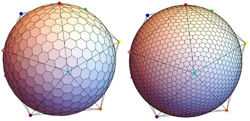
The OHQS encoding scheme of the planar hexagonal grid system has been established and extended on the surface of the icosahedron. The ISEA4H DGGS was constructed by Snyder equal-area projection. Figure 18 shows the third and fourth levels of the ISEA4H DGGS extended from the OHQS planar hexagonal grid system to the sphere. For the OHQS DGGS, the transformation algorithm between geographic coordinates and codes was realized and compared with the HLQT encoding scheme.

Figure 18. Third and fourth levels of extension of the icosahedron from the planar hexagonal grids

4.2.1 Transformation between geographic coordinates and codes

An experiment is designed to test the transformation between geographic coordinates and codes. The geographic coordinate $\left(B,L\right)$ was converted to codes in different DGGS resolutions. These codes obtained the geographic coordinates of the center point and six vertices of the hexagonal cells where the codes are located. These cells are displayed on the map. In this experiment, the center location of Beijing $\left({39.9177}^{\circ }N,{116.4126}^{\circ }E\right)$ was selected and transformed to codes from resolutions 5–12 in the OHQS. The results are shown in Table 7 and Figure 19.

Figure 19. Result of transformation from codes to geographic coordinates from resolutions 5–12

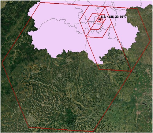
Table 7. ISEA4H OHQS codes at different resolutions

Level	Type of tile	Index of tile	Code	Center coordinate
5	Hg	1	11331	$\left({39.42}^{\circ }N,{115.96}^{\circ }E\right)$
6	Hg	1	321232	$\left({39.71}^{\circ }N,{116.66}^{\circ }E\right)$
7	Hg	1	1133113	$\left({39.89}^{\circ }N,{116.35}^{\circ }E\right)$
8	Hg	1	11331130	$\left({39.89}^{\circ }N,{116.35}^{\circ }E\right)$
9	Hg	1	321232122	$\left({39.93}^{\circ }N,{116.44}^{\circ }E\right)$
10	Hg	1	3212321222	$\left({39.91}^{\circ }N,{116.39}^{\circ }E\right)$
11	Hg	1	32123212202	$\left({39.92}^{\circ }N,{116.42}^{\circ }E\right)$
12	Hg	1	321232122020	$\left({39.92}^{\circ }N,{116.42}^{\circ }E\right)$

4.2.2 Comparison of the efficiency of transformation between geographic coordinates and codes

In this experiment, 1000 codes are randomly selected from each resolution to calculate the geographic coordinates of the center point and six vertices of the hexagonal cells, and 10000 geographic coordinates are randomly chosen to obtain the codes in different resolutions. The transformation efficiency of the OHQS and HLQT from resolution 5–12 was tested ten times, and the unit is $ms$. A comparison of the efficiency of transformation between OHQS and HLQT is shown in Figure 20 and Table 8.

Figure 20. Comparison of the efficiency of transformation between the HLQT and the OHQS

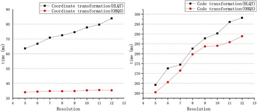
Table 8. Transformation time for experiments (ms)

res	Coordinate transformation		Code transformation
	HLQT	OHQS	HLQT	OHQS
5	63.6	34	264.2	260.5
6	66.7	34.4	272.6	265.6
7	70.9	34.8	274.5	271.5
8	72.5	34.7	282.6	279.7
9	74.6	34.8	287.8	283.7
10	77.8	35.3	290.3	284
11	79.7	35.5	296.1	285.9
12	83.9	35.3	298.2	288.9

The results show that the average efficiency of the OHQS from geographic coordinates to the code conversion algorithm is approximately 2 times that of the HLQT algorithm. As the resolutions increase, the efficiency of the OHQS remains basically the same. The conversion efficiency of the OHQS from codes to geographic coordinates is slightly higher than that of the HLQT, both of which are not greatly affected by the increase in resolution. The results are analyzed as follows:

1. The transformation efficiency in this paper is less affected by resolutions, and the transformation from coordinates to codes remains roughly unchanged because only one step in the algorithm involves the operation of the resolution, such as step 1 of algorithm 2 and step 5 of algorithm 3.

2. The HLQT uses the parallelogram rule to project the coordinates onto two specific coordinate axes. The corresponding component codes on the two axes are obtained, and the final code is calculated by the addition of component codes. The HLQT still implements the transformation by the addition operation. We directly realize the transformation from geographic coordinates to code through the mutual conversion of the $IJK$ coordinate system, $ij$ coordinate system and $ijk$ coordinate system. A substantial increase in efficiency has been achieved.

3. In the transformation from codes to geographic coordinates, the OHQS and HLQT are similar in efficiency, but the first symbol of the HLQT affects some computation time. Therefore, the transformation efficiency of the OHQS from code to geographic coordinates is slightly higher than that of the HLQT.

4.3 Multisource data fusion in the DGGS for rainstorm influences evaluation

Analyzing environmental processes such as hurricanes, wildfires, and rainstorms is ill-equipped for multisource geospatial data. DGGSs have been developed as a new solution for multisource spatial data processing and analysis. In this case, we use spatial data modeling on DGGSs to realize the fusion and analysis of multisource spatial data for the influence evaluation of the ‘Beijing 7.16’ rainstorm disaster. Figure 21 shows the process flow.

Figure 21. Schematic of the process flow of multisource data fusion on DGGS for rainstorm influence evaluation

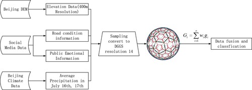
Figure 22. Distribution of rainstorm impacts in urban of Beijing on 16 and 17 July 2018

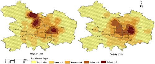
The multisource data are derived from analyzing the influences of the ‘Beijing 7.16’ rainstorm disaster. We obtained and processed social media data related to rainstorm disasters and extracted structured traffic impact information. In addition, there are elevation data, road network data, and climate data. Road condition information and public emotional information are point vector data; road network data is polyline vector data; and elevation data and average precipitation data of Beijing are raster data. We sampled all data into the 14th resolution grids using the method of spatial data modeling on a discrete global grid system. Next, a weight value is assigned to each influencing factor, and the comprehensive impact value of rainstorm disasters is calculated for each hexagonal grid. The natural breakpoint method is applied to divide each grid into five levels of rainstorm impact—highest risk, higher risk, moderate risk, lower risk and lowest risk—and the results are displayed. We effectively assessed the spatiotemporal distribution of rainstorm impacts in urban of Beijing on 16 and 17 July 2018, as shown in Figure 22.

5. Conclusion

This study establishes the vector model of the aperture 4 hexagonal grid system, and designs the encoding scheme of an optimized hexagonal quadtree structure (OHQS) by translation transformation. Compared with the complex first symbol of the HLQT and the mixture of two types of encoding of the HQBS, the quadtree encoding in this paper is more concise. In the code addition and adjacent grid retrieval operations, in addition to constructing a set of addition rules based on induction, we also constructed a set of addition rules based on $ijk$ coordinate transformation. The results show that the OHQS encoding operation is more efficient and that the encoding operation based on the $ijk$ coordinate system is faster than the encoding operation based on the induction and addition table. We realize the transformation from geographic coordinates to codes through the mutual conversion of the $IJK$ coordinate system, $ij$ coordinate system and $ijk$ coordinate system, which is twice as efficient as the transformation based on code addition. These findings can provide an alternative for other types of DGGS operations. In addition, we also employed OHQS to realize traditional spatial data modeling on the DGGS, which provided the basis for multisource data fusion and analysis, and realized the impact analysis of the ‘Beijing 7.16’ rainstorm disaster. This study provides solutions for the application of the DGGS to traditional spatial data.

Disclosure statement

No potential conflict of interest was reported by the author(s).

Additional information

Funding

This work is supported by the Strategic Priority Research Program of Chinese Academy of Sciences [grant number XDA19020201].

Appendices

1. For any $n\ge 0$ and $P_i\in P_n$, there exists a unique $d_i\in \left\{0,{\displaystyle \frac{1}{2^i}\mathit{u},{\displaystyle \frac{1}{2^i}\mathit{v},{\displaystyle \frac{1}{2^i}\left(-\mathit{u}-\mathit{v}\right)}}}\right\}$, $\begin{array}{c}{P}_i=\sum _{i=1}^n{d}_i\end{array}$

Proof.

$P_n=P_{n-1}+{\displaystyle \frac{1}{2^{n-1}}D}$ $=P_{n-2}+{\displaystyle \frac{1}{2^{n-2}}D+{\displaystyle \frac{1}{2^{n-1}}D}}$ $=P_0+D+{\displaystyle \frac{1}{2}D+\cdots +{\displaystyle \frac{1}{2^{n-2}}D+{\displaystyle \frac{1}{2^{n-1}}D}}}$ $=P_0+\sum _{i=1}^n{\displaystyle \frac{1}{2^{i-1}}D}$ $=P_0+\sum _{i=1}^n\left\{0,{\displaystyle \frac{1}{2^{i-1}}\mathit{u},{\displaystyle \frac{1}{2^{i-1}}\mathit{v},{\displaystyle \frac{1}{2^{i-1}}\left(-\mathit{u}-\mathit{v}\right)}}}\right\}$For $p_n\in P_n,p_n=\sum _{i=1}^n{d}_i$

1. For the code in the lower right corner, the excess hexagonal grids can be expressed as: (4) $\begin{array}{c}R{L}_n=\left(2^{n-1}+n_1\right){\mathit{u}}_{\mathit{n}}+n_2{\mathit{v}}_{\mathit{n}};2n_1-n_2>2,n_1,n_2\in Z\mathrm{\#};\end{array}$(4)

The set of hexagonal grids in the upper left corner can be expressed as: (5) $\begin{array}{c}R{L}_n^{\ast }=(2^{n-1}+n_1){\mathit{u}}_{\mathit{n}}^{\ast }+n_2{\mathit{v}}_{\mathit{n}}^{\ast };2n_1-n_2>2,n_1,n_2\in Z\end{array}$(5) $\mathit{u}<=>{\mathit{u}}_{\mathit{n}}^{\ast }$, $\mathit{v}<=>{\mathit{v}}_{\mathit{n}}^{\ast }$, then $R{L}_n<=>R{L}_n^{\ast }$.

Proof.

We construct $P_n$ and $P_n^{\ast }$ as shown in the figure. The lattices on the red line in the lower right corner of $P_n$ and $P_n^{\ast }$ satisfy $2n_1-n_2-2=0$, and the lattices outside the red line satisfy $2n_1-n_2-2>0$. Therefore, $R{L}_n=\mathit{u}+n_1{\mathit{u}}_{\mathit{n}}+n_2{\mathit{v}}_{\mathit{n}}=\left(2^{n-1}+n_1\right){\mathit{u}}_{\mathit{n}}+n_2{\mathit{v}}_{\mathit{n}};2n_1-n_2>2$. Similarly, $R{L}_n^{\ast }={\mathit{u}}^{\mathbf{\ast }}+n_1{\mathit{u}}_{\mathit{n}}^{\ast }+n_2{\mathit{v}}_{\mathit{n}}^{\ast }=(2^{n-1}+n_1){\mathit{u}}_{\mathit{n}}^{\ast }+n_2{\mathit{v}}_{\mathit{n}}^{\ast };2n_1-n_2>2$. $P_n<=>P_n^{\ast }$, ${\mathit{u}}_{\mathit{n}}<=>{\mathit{u}}_{\mathit{n}}^{\ast }$, ${\mathit{v}}_{\mathit{n}}<=>{\mathit{v}}_{\mathit{n}}^{\ast }$, and then $L_n<=>L_n^{\ast }$.

3) Formula 9: $\left(\begin{array}{c}\begin{array}{c}i\\ j\end{array}\\ k\end{array}\right)=\sum _{r=1}^n\left\{{\left(\begin{array}{cc}\begin{array}{c}\begin{array}{cc}2& 0\\ 0& 2\end{array}\\ \begin{array}{cc}0& 0\end{array}\end{array}& \begin{array}{c}0\\ 0\\ 2\end{array}\end{array}\right)}^{n-r+1}\cdot \phi \left(a_r\right)\right\}$

Proof.

For the r-th digit $a_r$ in the OHQS code $\alpha =a_1{a}_2....a_n$, if $a_r=1$, the corresponding vector is ${\displaystyle \frac{1}{2^{r-1}}\mathit{v}=2^{n-r+1}{\mathit{v}}_{\mathit{n}}}$, and the corresponding value in the ijk coordinate system is $(i,j,k{)}_r=(0,2^{\mathit{n}-\mathit{r}+1},0)$; if $a_r=2$, the corresponding vector is ${\displaystyle \frac{1}{2^{r-1}}\left(-\mathit{v}-\mathit{u}\right)=2^{n-r+1}(-{\mathit{v}}_{\mathit{n}}-{\mathit{u}}_{\mathit{n}})}$, and the corresponding value in the ijk coordinate system is $(i,j,k{)}_r=(0,,0,2^{\mathit{n}-\mathit{r}+1})$; if $a_r=3$, the corresponding vector is ${\displaystyle \frac{1}{2^{r-1}}\mathit{u}=2^{n-r+1}{\mathit{u}}_{\mathit{n}}}$, and the corresponding value in the ijk coordinate system is $(i,j,k{)}_r=(2^{\mathit{n}-\mathit{r}+1},0,0)$. This result leads to $\left(\begin{array}{c}\begin{array}{c}i\\ j\end{array}\\ k\end{array}\right)=\sum _{r=1}^n\left\{{\left(i,j,k\right)}_r\right\}=\sum _{r=1}^n\left\{{\left(\begin{array}{cc}\begin{array}{c}\begin{array}{cc}2& 0\\ 0& 2\end{array}\\ \begin{array}{cc}0& 0\end{array}\end{array}& \begin{array}{c}0\\ 0\\ 2\end{array}\end{array}\right)}^{n-r+1}\cdot \phi \left(a_r\right)\right\}$

References

- Adams, Benjamin. 2017. “Wāhi, a Discrete Global Grid Gazetteer Built Using Linked Open Data.” International Journal of Digital Earth 10 (5): 490–503.
- Alborzi, Houman, and Hanan Samet. 2000. Augmenting SAND with a Spherical Data Model. Paper presented at the first International conference on Discrete Global Grids. santa barbara, California, March.
- Amiri, Ali Mahdavi, Faraz Bhojani, and Faramarz Samavati. 2013. One-to-two digital earth. Paper presented at the International Symposium on Visual Computing.
- Amiri, Ali Mahdavi, Faramarz Samavati, and Perry Peterson. 2015. “Categorization and Conversions for Indexing Methods of Discrete Global Grid Systems.” ISPRS International Journal of Geo-Information 4 (1): 320–336.
- Bauer-Marschallinger, Bernhard, Daniel Sabel, and Wolfgang Wagner. 2014. “Optimisation of Global Grids for High-Resolution Remote Sensing Data.” Computers & Geosciences 72: 84–93.
- Ben, J., X. C. Tong, C. H. Zhou, and K. X. Zhang. 2015. “Construction Algorithm of Octahedron Based Hexagon Grid Systems.” J. Geo-Inf. Sci 6: 54–61.
- Bresenham, Jack. 1977. “A Linear Algorithm for Incremental Digital Display of Circular Arcs.” Communications of the ACM 20 (2): 100–106.
- Cheng, Yuqi, Le Yu, Yuanyuan Zhao, Yidi Xu, Kwame Hackman, Arthur P Cracknell, and Peng Gong. 2017. “Towards a Global oil Palm Sample Database: Design and Implications.” International Journal of Remote Sensing 38 (14): 4022–4032.
- Craglia, Max, Kees de Bie, Davina Jackson, Martino Pesaresi, Gábor Remetey-Fülöpp, Changlin Wang, Alessandro Annoni, Ling Bian, Fred Campbell, and Manfred Ehlers. 2012. “Digital Earth 2020: Towards the Vision for the Next Decade.” International Journal of Digital Earth 5 (1): 4–21.
- Dutton, Geoffrey. 1984. “Part 4: Mathematical, Algorithmic and Data Structure Issues: Geodesic Modelling of Planetary Relief.” Cartographica: The International Journal for Geographic Information and Geovisualization 21 (2-3): 188–207.
- Dutton, Geoffrey. 1999. “Scale, Sinuosity, and Point Selection in Digital Line Generalization.” Cartography and Geographic Information Science 26 (1): 33–54.
- Goodchild, Michael F. 2018. “Reimagining the History of GIS.” Annals of GIS 24 (1): 1–8.
- Guo, Huadong. 2017. “Big Earth Data: A new Frontier in Earth and Information Sciences.” Big Earth Data 1 (1-2): 4–20.
- Guo, Huadong, Zhen Liu, Hao Jiang, Changlin Wang, Jie Liu, and Dong Liang. 2017. “Big Earth Data: A new Challenge and Opportunity for Digital Earth’s Development.” International Journal of Digital Earth 10 (1): 1–12.
- Guo, Huadong, Lizhe Wang, Chen Fang, and Liang Dong. 2014. “Scientific big Data and Digital Earth.” Chinese Science Bulletin 59 (35): 5066–5073.
- Iii, Bartholdi, J. John, and Paul Goldsman. 2001. “Continuous Indexing of Hierarchical Subdivisions of the Globe.” International Journal of Geographical Information Science 15 (6): 489–522.
- Jendryke, Michael, and Stephen C McClure. 2021. “Spatial Prediction of Sparse Events Using a Discrete Global Grid System; a Case Study of Hate Crimes in the USA.” International Journal of Digital Earth 14 (6): 1–17.
- Jin, B., L. I. Yalu, C. H. Zhou, R. Wang, and D. U. Lingyu. 2018. “Algebraic Encoding Scheme for Aperture 3 Hexagonal Discrete Global Grid System.” SCIENCE CHINA Earth Sciences 61 (002): 215–227.
- Kimerling, Jon A, Kevin Sahr, Denis White, and Lian Song. 1999. “Comparing Geometrical Properties of Global Grids.” Cartography and Geographic Information Science 26 (4): 271–288.
- Li, Shuang, Guoliang Pu, Chengqi Cheng, and Bo Chen. 2019. “Method for Managing and Querying geo-Spatial Data Using a Grid-Code-Array Spatial Index.” Earth Science Informatics 12 (2): 173–181.
- Li, M., E. Stefanakis, and H. Mcgrath. 2020. National Terrain Data Management on Discrete Global Grids in Canada. Paper presented at the AutoCarto2020.
- Lin, Bingxian, Liangchen Zhou, Depeng Xu, A-Xing Zhu, and Guonian Lu. 2018. “A Discrete Global Grid System for Earth System Modeling.” International Journal of Geographical Information Science 32 (4): 711–737.
- Ma, Yue, Guoqing Li, Xiaochuang Yao, Qianqian Cao, Long Zhao, Shuang Wang, and Lianchong Zhang. 2021. “A Precision Evaluation Index System for Remote Sensing Data Sampling Based on Hexagonal Discrete Grids.” ISPRS International Journal of Geo-Information 10 (3): 194–194.
- Mahdavi-Amiri, Ali, Troy Alderson, and Faramarz Samavati. 2015. “A Survey of Digital Earth.” Computers & Graphics 53: 95–117.
- Mocnik, Franz-Benjamin. 2019. “A Novel Identifier Scheme for the ISEA Aperture 3 Hexagon Discrete Global Grid System.” Cartography and Geographic Information Science 46 (3): 277–291.
- Peterson, Perry.. 2011. "Close-packed uniformly adjacent, multiresolutional overlapping spatial data ordering." In.: U.S. Patent No. 8,018,458. 13 Sep. 2011.
- Peterson, Perry R.. 2016. “Discrete Global grid systems.” International Encyclopedia of Geography: People, the Earth, Environment and Technology 2016: 1–10.
- Purss, M., R. Gibb, F. Samavati, P. Peterson, J. Rogers, J. Ben, and C. Dow. 2017. Topic 21: Discrete Global Grid Systems Abstract Specification.” Open Geospatial Consortium: Wayland, MA, USA.
- Robertson, Colin, Chiranjib Chaudhuri, Majid Hojati, and Steven A Roberts. 2020. “An Integrated Environmental Analytics System (IDEAS) Based on a DGGS.” ISPRS Journal of Photogrammetry and Remote Sensing 162: 214–228.
- Sahr, Kevin. 2005. Discrete global grid systems: a new class of geospatial data structures.” University of Oregon.
- Sahr, Kevin. 2008. “Location Coding on Icosahedral Aperture 3 Hexagon Discrete Global Grids.” Computers, Environment and Urban Systems 32 (3): 174–187.
- Sahr, Kevin. 2011. “Hexagonal Discrete Global Grid Systems for Geospatial Computing.” Archiwum Fotogrametrii, Kartografii i Teledetekcji 22: 363–376.
- Sahr, Kevin, Denis White, and A. Jon Kimerling. 2003. “Geodesic Discrete Global Grid Systems.” Cartography and Geographic Information Science 30 (2): 121–134.
- Shuang, L. I., C. H. E. N. G. Chengqi, T. O. N. G. Xiaochong, C. H. E. N. Bo, and Z. H. A. I. Weixin. 2016. “A Study on Data Storage and Management for Massive Remote Sensing Data Based on Multi-Level Grid Model.” Acta Geodaetica Et Cartographica Sinica 45 (S1): 106–114.
- Snyder, John P. 1992. “An Equal-Area map Projection for Polyhedral Globes.” Cartographica: The International Journal for Geographic Information and Geovisualization 29 (1): 10–21.
- Tong, Xiaochong, Ben Jin, Wang Ying, Yongsheng Zhang, and Pei Tao. 2013. “Efficient Encoding and Spatial Operation Scheme for Aperture 4 Hexagonal Discrete Global Grid System.” International Journal of Geographical Information Science 27 (5-6): 898–921.
- Vince, Andrew. 2006. “Indexing the Aperture 3 Hexagonal Discrete Global Grid.” Journal of Visual Communication and Image Representation 17 (6): 1227–1236.
- Vince, Andrew, and Xiqiang Zheng. 2009. “Arithmetic and Fourier Transform for the PYXIS Multi-Resolution Digital Earth Model.” International Journal of Digital Earth 2 (1): 59–79.
- Wang, R., J. Ben, L. Y. Du, J. B. Zhou, and Z. X. Li. 2019. The code operation scheme for the icosahedral aperture 4 hexagon grid system.” Geomat. Inf. Sci. Wuhan Univ.
- Wang, R., J. Ben, J. B. Zhou, and M. Y. Zheng. 2021. “A Generic Encoding and Operation Scheme for Mixed Aperture Three and Four Hexagonal Discrete Global Grid Systems.” International Journal of Geographical Information Science 35 (3): 513–555.
- Wang, Rui, Du Jin Ben, Jianbin Zhou, and Zhuxin Li. 2018. “Encoding and Operation for the Planar Aperture 4 Hexagon Grid System.” Acta Geodaetica Et Cartographica Sinica 47 (7): 1018–1025.
- White, Denis. 2000. “Global Grids from Recursive Diamond Subdivisions of the Surface of an Octahedron or Icosahedron.” Environmental Monitoring and Assessment 64 (1): 93–103.
- Yao, Xiaochuang, Guoqing Li, Junshi Xia, Jin Ben, Qianqian Cao, Long Zhao, Yue Ma, Lianchong Zhang, and Dehai Zhu. 2020. “Enabling the big Earth Observation Data via Cloud Computing and DGGS: Opportunities and Challenges.” Remote Sensing 12 (1): 83–83.
- Zhao, Xuesheng, Jun Chen, and Zhilin Li. 2006. An Efficient Method for Transformation Between QTM Codes and Geographic Coordinates. Paper presented at the Geoinformatics 2006: GNSS and Integrated Geospatial Applications.
- Zheng, Xiqiang. 2007. Efficient Fourier transforms on hexagonal arrays.” University of Florida.