Deep learning for land use and land cover classification from the Ecuadorian Paramo.

ABSTRACT

The paramo, plays an important role in our ecosystems as They balance the water resources and can retain substantial quantities of carbon. This research was carried out in the province of Tungurahua, specifically the Quero district.

The aim is to develop a classification of the land use land cover (LULC) in the paramo using satellite imagery using several classifiers and determine which one obtains the best performance, for which three different approaches were applied: Pixel-Based Image Analysis (PBIA), Geographic Object-Based Image Analysis (GEOBIA), and a Deep Neural Network (DNN). Various parameters were used, such as the Normalized Difference Vegetation Index (NDVI), the Bare Soil Index (BSI), texture, altitude, and slope. Seven classes were used: paramo, pasture, crops, herbaceous vegetation, urban, shrubrainland, and forestry plantations. The data was obtained with the help of onsite technical experts, using geo-referencing and reference maps. Among the models used the highest-ranked was DNN with an overall precision of 87.43%, while for the paramo class specifically, GEOBIA reached a precision of 95%.

KEYWORDS:

• Classification
• land use and land cover
• pixel-based image analysis
• geographic object-based image analysis
• deep neural network

1. Introduction

The paramo is a neotropical alpine wetland ecosystem, approximately covering the high Andean region of Venezuela, Colombia, and Ecuador, with a few more outcrops in the north towards Costa Rica and Panama and towards the south in northern Peru (Hofstede and Perez 1996; Hofstede, Segarra and Mena 2003), they have located at 3,500 meters above sea level (masl) and despite their isolated location, these ecosystems are of major importance in the social and economic arenas (Buytaert et al. 2012). Around 5,000 different species of plants and endemic vegetation can be found in the paramo comprising mainly pastureland, espeletia rosettes, dwarf Shrubs, cushion plants and espeletia giant rosettes (Hofstede, Chilito and Sandovals 1995; Vargas and Zuluaga 1986; Beltran 2009) and they are the home of several animal species, such as condors and bears, which are in danger of extinction. Moreover, they are a permanent and bountiful supply of good quality water for domestic, irrigation, industrial, and even electricity generating purposes (Celleri and Feyen 2009; Buytaert et al. 2006).

It is important for carbon storage since by accumulating a large amount of organic matter, it helps mitigate global warming, in addition to being the livelihood of many families (Hofstede, Segarra, and Mena 2003; Minaya et al. 2015; Farley et al. 2004).

In Ecuador, paramo is undergoing an uncontrollable process of deterioration caused by human activity such as sheep and cattle grazing; farmers benefit from the razing of herds through the removal of the dead straw so that the re-sprouting grass provides fresh pasture for their livestock to feed on, they also burn the paramo to prepare it for cultivation, even for beliefs or mythical reasons such as making fire to attract rain (Hofstede et al. 2014). The paramo covers approximately 6.1% of the surface of Ecuador, accounting for 1,515,273 ha. However, between 1990 and 2016 roughly 51,000 ha of moorland were lost (Teran et al. 2019). Currently, the use of satellite images is the most cost-effective and fastest way to perform LULC classification over large areas. In Ecuador, few classifications have been made in the paramo ecosystems, attributing to the fact that the Andean areas are difficult to access due to their topography and the altitude at which they are located, in addition to the fact that they generally remain covered with clouds (Colby & Keating. 1998; Martinuzzi et al. 2007; Curatola Fernández et al. 2015; Ayala-Izurieta et al. 2017).

So far, few LULC classifications have been made in the paramo such as the one presented by a supervised maximum likelihood algorithm that determines the rate of soil carbon loss from traditional fallow agriculture, besides, measuring the change in agricultural areas between 1991 and 2017 and understand the patterns of land use in the Northern Andes and determine the impact on carbon storage in land use (Thompson et al. 2021).

In another study, land cover change was evaluated in the herbaceous paramo of central Ecuador using Landsat 8 images using Object-Based Image Analysis (OBIA) and a Classification and Regression Tree algorithm (CART) to determine the loss of the herbaceous and anthropogenic paramo in this area (García et al. 2019). LULC classification is important for monitoring the changes taking place due to the intrusion of farmers and which have an impact on the ecosystem.

With this information, environmental management plans can be drawn up to take positive action to foster conservation and regeneration in the paramo.

The purpose of this study was to carry out LULC classification in the province of Tungurahua, Quero district and the surrounding areas using three methods: PBIA, GOBIA, and DNN adding different characteristics such as NDBI, BSI, texture, altitude, and slope. The analysis focused on determining the level of accuracy when using satellite imagery in this type of region.

To date, no research has been carried out comparing the performance of different classifiers in the mapping of the paramo, nor the implementation of an artificial neural network algorithm for these areas.

The difficult access to the places can be an important factor that affects the LULC classification in the cloud zone (Colby & Keating 1998; Martinuzzi et al. 2007; Curatola Fernández et al. 2015), the lack of reference maps or that they are very old, the little information of studies carried out is one of the limitations to carry out classifications in the moor.

It is necessary to evaluate the LULC classification in the paramo efficiently, and quickly, in order to have a better understanding of the causes that influence the loss of the paramo, and that the corresponding institutions can act on time, to save this ecosystem.

2. Materials and methods

2.1. Study area

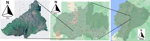
The study area covers an area of ⁣⁣173.81 km2, which represents 5% of the territory of the province of Tungurahua, at coordinates 1° 22’ 35'’ South Latitude and 78° 36'21'’ West Longitude (Figure 1), the altitude of the territory of the district ranges from 2,760 m.a.s.l, with an average altitude of 3,038 m.a.s.l and reaches up to 4,500 meters above sea level in the paramo. This phenomenon allows temperatures to be recorded on average of 10 - 12 degrees C ° (see Figure 1).

Figure 1. Geographical location of the Quero distric in the Ecuadorian highlands.

The main activity of the district is agriculture, forestry, and livestock, which represents 66.96% of the economic activities to which its inhabitants are dedicated; due to this peculiarity, several productive activities are carried out in the high area's activities such as livestock are used, since the climate and its characteristics allow the planting of grass. Short-cycle crops such as potatoes and onions are planted in the middle zone where the boundary zone with the paramo begins and in the lower zone broad beans, carrots, and peas, among others.

2.2. Data

This was obtained using Google Earth Engine (GEE), a cloud-based platform that enables access to satellite images which can then be quickly processed (Gorelick et al. 2017). Sentinel 2A images with a resolution of 10  m and a temporal frequency of 10 days were used, these provide 13 different bands that are orthorectified with refraction levels below the atmosphere, which allows them to be more realistic and sharp, they were obtained from the repository from GEE ee.ImageCollection bank (COPERNICUS/S2 SR). To carry out the classification generated a composite image of images that were filtered according to the region of interest, in this case, the Quero district, with a start and end date from 01-01-2020–12-31-2020, a percentage of cloud cover of no more than 20%, cloud masking is also used by a function created in GEE using the QA band, which is a bitmask band with cloud mask information. Later, it was obtained a medium pixel image for the selected bands of the mosaic of images that meet these conditions to add to this composition the NDVI that is related to the amount of chlorophyll concentrated in the leaves and the variations in biomass productivity (Polykretis et al. 2020). For the calculation, the following formula is used: (1) $NDVI={\displaystyle \frac{NIR-RED}{NIR+RED}}$(1) Where: NIR (Near Infrared) = band 8, RED =  band 4

As well as this the BSI (Bare Soil Index) was obtained, which is used principally to differentiate agricultural land from bare or fallow land, generating a final compound data set. BSI is obtained using the following formula: (2) $BSI={\displaystyle \frac{GREEN+NIR}{GREEN-NIR}}$(2) Where: NIR =  band 8, GREEN =  band 3

The initial composition of the resulting image includes bands B1, B2, B3, B4, B5, B6, B7, B8, B8A, B9, B11, B12, QA10, QA20, QA60, NDVI, BSI, which will be used as input data for the classification algorithms.

3. Methodology

3.1. Classification

With the aim of determining which is the best method for classification in the paramo three different approaches were developed, with distinct input parameters. The following options were used:

• PBIA includes NDVI and BSI indices.

• PBIA includes NDVI and BSI indices, as well as altitude and slope information.

• GEOBIA includes NDVI and BSI indices and texture information.

• GEOBIA includes NDVI and BSI indices as well as texture, altitude, and slope information.

• DNN includes spectrum bands as well as NDVI and BSI indices.

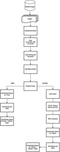
For the classification, seven classes of training points were selected: paramo, pasture, crops, herbaceous vegetation, urban, shrub, and forestry plantations (see Figure 2). This was conducted with the help of visual interpretation with local experts using georeferencing with Global Positioning Systems (GPS), orthophotos, Google Earth Pro, and classification reference maps (Teran et al. 2019). For the PBIA and GEOBIA, the methodology shown in Figure 3 was used.

Figure 2. Distribution of samples of the seven classes to classify.

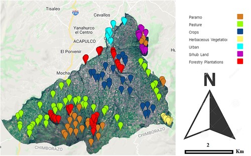
Figure 3. Methodology for pixel and object-based classification using GEE.

3.1.1. Pixel-Based Image Analysis with NDVI and BSI

In GEE, the PBIA is performed using the composite image created previously, which includes spectral bands typical of the Sentinel-2 B1-B12 image, in addition to the NDVI and BSI spectral indices. In this type of classification, the pixels use their spectral information to compare themselves with the spectral signatures of the LULC classes of the training data.

Random Forest (RF) is a supervised classification method it is built based on many decision trees, it requires two adjustment parameters such as the number of trees (ntree) and the number of variables in each division (mtry). It has been shown to be highly effective with the use of satellite images (Gislason et al. 2006; Amani et al. 2017; Mi et al. 2019; Talukdar et al. 2020; Umarhadi et al. 2022).

RF provides a metric of varying importance, is resistant to outliers, and is capable of handling high-dimensional data and uncovering nonlinear relationships (Breiman 2001). RF uses bootstrap aggregation (bagging) to build multiple decision trees, it also has a great ability to discriminate variables that are not very relevant it has been determined that increasing the size of the trees does not increase the performance of this algorithm, rather it only increases the capacity computational required when the number of trees reaches a certain threshold (Oshiro et al. 2012), GEE can analyze the number of trees needed to reach instances out-of-bag with which it was determined that the optimal number of trees is 50 mtry, was set to the square root of the input variables, once this algorithm was applied classified image is obtained to which a morphological operation reduction to minimize the salt and pepper effect.

3.1.2. Pixel based Image Analysis with nDVI, BSI, altitude and slope

This classification is also based on pixels; apart from the indexes already indicated elevation and slope information is added to improve the classification because the moors are over 3500  m.a.s.l, these data were obtained from the repository SRTMGL1_003 produced by the Shuttle Radar Survey Mission(SRTM) that generated the first totally free Digital Elevation Model (DEM), almost globally they have a spatial resolution of 30  m and an altitude accuracy of 16  m (Farr et al. 2007) these data are found available at GEE. This dataset differs from other versions because it has been gap-filled with open-source data, and not with commercial applications or in other cases that continue to have inconsistencies.

In the same way, to perform the classification, a GEE RF algorithm is used, with several trees of 50 established with the methods described above morphological operation to reduce the salt and pepper effect.

3.2. Geographic Object-Based Image Analysis

3.2.1. Geographic Object-Based Image Analysis with nDVI, BSI, and texture

Texture is an important feature used in the identification of objects or regions in an image. In the 70s, 14 measures of texture were proposed based on the spatial dependence of grey tones (Haralick et al. 1973). The use of texture in an image is done visually, but it can be measured mathematically utilizing the grey level co-occurrence matrix or for its acronym in English GLCM (Grey Level Co-occurrence Matrix). GLCM has become a method of obtaining features in remote sensing data (Ozdemir et al. 2008) and has been used, for instance, to estimate the structure of the tropical forest (Castillo-Santiago et al. 2010)and land cover classification (Wan & Chang, 2018; Jin et al. 2018).

Seven GLCM metrics suggested by (Hall-Beyer 2017) were used which were: second angular momentum (ASM), contrast, correlation, entropy, difference, inverse differential momentum (IDM), and average sum (SAVG).

For the conversion of RGB image to grayscale, the equation proposed by (Ge & Liu, 2020) was used, using the bands B3, B4, B5 and thus generating the input for GLCM as follows: (3) $\mathrm{Gray}=(0.3\times \mathrm{B}5)+(0.59\times \mathrm{B}4)+(0.11\times \mathrm{B}3)$(3) A Principal Components Analysis (PCA) was then applied to obtain a single representative band (the first PC) that usually contains the largest amount of contextual information. Next, select the clusters band from the output of the Simple Non-Iterative Clustering (SNIC), and the PC1 taken from the PCA data is added and the average of each segment is calculated concerning that group.

SNIC algorithm improves computational efficiency, memory consumption, and segmentation quality compared to the Simple Linear Iterative Clustering (SLIC) algorithm (Achanta & Susstrunk, 2017). Initializes the pixels from the centroid in a regular image grid, based on this centroid determines the dependency of each pixel using its five-dimensional color distance and spatial coordinates, uses these distances to produce effective, compact, and approximately uniform super pixels. The parameters of the SNIC algorithm are the following: “compactness factor”; It affects the clusters’ shape while these values are higher the compacts are clusters, “connectivity” defines the contiguity type to merge adjacent groups and “neighborhood size” to avoid mosaic boundary artifacts.

Considering the characteristics of the area, and carrying out experiments with the parameters, they were established as follows: a compactness factor of 0, connectivity of 8, and a neighborhood size of 16.

To carry out the GEOBIA, it is taken as a reference the algorithm proposed by (Tassi & Vizzari, 2020); where the Gray Level Co-occurrence Matrix (GLCM) is merged with the SNIC algorithm, in addition to applying a component analysis that simplifies a band of texture information, the classification is done using an RF algorithm.

3.2.2. Geographic Object-Based Image Analysis with nDVI, BSI, texture, altitude, and slope

As in the preliminary classification, the object-based methodology is used with NDVI, BSI, and texture indices, to which the slope and altitude are added also using the DEM data with an RF algorithm with several trees of 50 obtained in the same way as in the previous examples, a new classification is obtained.

3.3. Deep Neural Network based classification

Figure 4 shows the steps to follow to perform the LULC classification in the moors using deep learning through DNN. The following classification was done in a cloud environment using a combination of GEE with TensorFlow, Google Collaborative, and Google Cloud Storage (GCS).

Figure 4. The methodology used for the LULC classification is a DNN.

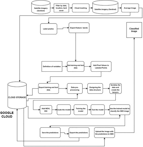
An image is created in GEE filtered with the same criteria: date, region of interest, and the same degree of cloudiness, adding part of the spectral bands typical of the Sentinel 2 images, the NDVI and BSI indices, this base image is stored in a CGS repository.

The training and test data are divided by 70% and 30% respectively. The data is processed so that they can have a suitable format and be read by the tensors, and the image to be classified is exported from the GEE assets base, storing them in GCS.

Neural networks are based on biological networks represented by a mathematical structure. They are mainly used to solve non-linear problems, they learn, memorize and generalize complex problems, they generally have three layers: input, output, and hidden layers.

Sentinel surface reflectance images, bands 1-12, are used as input data, in the same way, that in the previous examples a filter is performed by coverage, area, and date with a percentage of cloudiness that does not exceed 20%, also performs a cloud masking to subsequently obtain a medium pixel image, these data are labelled with the respective classes with coverage points of the seven classes to be classified that are exported from GEE to a repository. Each labelled point has a property that defines the type of class to which it belongs, then the points are superimposed on the images to obtain predictor variables together with the labels; additional features are added in this case the NDBI and BSI.

Next, a DNN is implemented that consists of an input of 64 neurons, two intermediate layers of, 32, and 16 neurons respectively, with a batch size of 16 with an activation function relu, a dropout of 0.2 between each layer to avoid overfitting; a softmax output function to that discriminates the seven characteristics for each of the coverages as an optimizer was used and as a metric the accuracy as a loss function, the cross-entropy was used. The model was trained for 1232 epochs as shown in Figure 5.

Figure 5. The architecture of the DNN to carry out the LULC classification in the paramo.

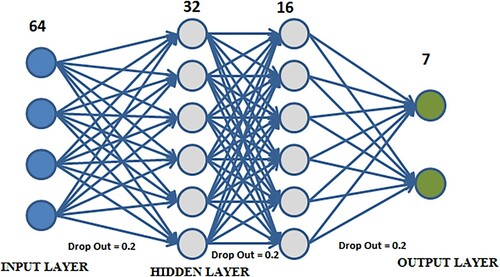
The number of neurons in each layer was selected by trial error tests until reaching the optimal values. Subsequently, using the resulting model predictions on the image that was stored in GCS, these predictions are exported to the GEE repository to be displayed.

4. Results

To determine the classification accuracy of the presented models, the overall accuracy was taken into account, which is measured by dividing the total number of correctly labelled samples by the total number of test samples. It was also evaluated using the kappa coefficient, which indicates the degree of agreement between the real field data and the predicted values. To measure the accuracy of each of the classes in the different classifications, the F1-Score metric was used, which indicates the relationship between accuracy and completeness.

In the present investigation, three methods of LULC classification were analysed in the paramo and its surroundings, it is observed that the classification utilizing a DNN obtains the best results at a general level, followed by the GEOBIA with NDVI, BSI, altitude and slope, obtaining a kappa index of more than 80%.

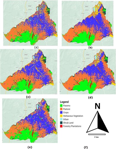
For data validation, one hundred data points were used for each class. Through a confusion matrix, the omission errors are obtained, which are the elements of a class that do not appear in it; and commission errors which are elements that do not belong to a class and appear in it. The map classifications with their respective legend is shown in Figure 6.

Figure 6. (a) PBIA+ NDVI +BSI, (b) PBIA + NDVI + BSI + Altitude + Slope (c), GEOBIA + NDVI + BSI + Texture, (d) GEOBIA + NDBI + BSI + Texture + Altitude + Slope, (E) Sorting by RNN, (f) LULC Classification Legend.

Figures 7–11 show the results obtained from the precision of the classifications obtained through confusion matrices.

Figure 7. Omission error, commission error, overall precision for PBIA + NDVI +BSI.

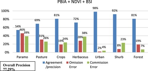
Figure 8. Omission error, commission error, overall precision for PBIA + NDVI +BSI + altitude + slope.

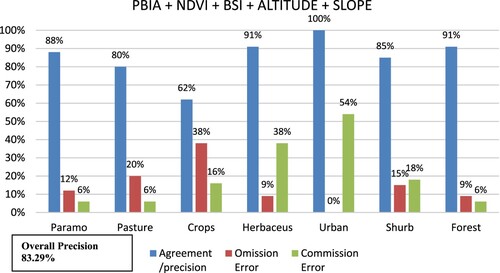
Figure 9. Omission error, commission error, overall precision for GEOBIA + NDVI + BSI + texture.

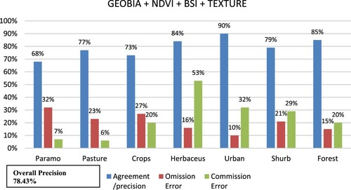
Figure 10. Omission error, commission error, overall precision for GEOBIA + NDVI + BSI + texture + altitude + slope.

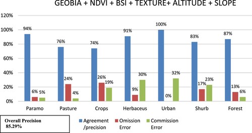
Figure 11. Omission error, Commission error, overall precision for classification using DNN + NDVI + BSI.

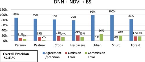
Table 1 shows the summary of the general accuracy and the kappa index for each of the classifications made in this study. The best results were obtained for DNN with an overall precision of 87.43% and a kappa index of 86.96%, then the GEOBIA with NDVI, BSI, texture, altitude, and slope with an overall precision of 85.29%, and a kappa index of 84.74%, followed by the PBIA with texture, altitude and slope with a general accuracy of 83.29% and a kappa index of 86.67%, then the GEOBIA with a general accuracy percentage of 78.43% and a kappa index of 77.63%, leaving back to PBIA with an overall accuracy of 77.29% and a kappa index of 73.44%.

Table 1. General accuracy indices and kappa of the PBIA, GEOBIA and DNN approaches.

	PBIA +NDVI + BSI	GEOBIA + NDVI + BSI + Texture	PBIA +NDVI + BSI + Texture + Altitude + Slope	GEOBIA +NDVI + BSI + Texture + Altitude+ Slope	Deep Neural Network
Overall Accuracy	77.29%	78.43%	83.29%	85.29%	87.43%
Kappa Index	76.44%	77.63%	82.67%	84.74%	86.96%

Then, the highest values of omission and commission errors for each classifier in the classes are shown below.

In the PBIA + NDBI + BSI, there are 46% omission errors in the paramo class and 39% commission errors for this same class, also for the pasture class there are 28% omission errors and 38% commission errors.

In PBIA + NDVI + BSI + altitude+ slope there are commission errors with 54% in the urban class, also 38% of commission errors in the herbaceous class, and 38% of commission errors in the crop class.

GEOBIA + NDVI + BSI + texture, presents omission errors of 32% in the paramo class, commission errors of 53% in the herbaceous class, and 32% of commission errors in the urban class.

GEOBIA + NDBI + BSI + texture + altitude + slope, presents commission errors in the herbaceous class of 30%, commission errors with 32% in the urban class.

The PBIA + NDVI + BSI with the PBIA + NDBI + BSI + altitude + texture + slope, shows the confusion of pixels in the herbaceous classes with the crop class, and also in the moorland class with the pasture and crop class. The PBIA and the GEOBIA are similar to each other. The PBIA with the GEOBIA + altitude + texture + slope have differences, especially in the moorland class, which is confused with the crops and pasture classes. The PBIA with the DNN has confusion mainly in the moorland class with the crop and pasture class, in addition to the fact that the herbaceous class with the forest class is similarly confused.

The PBIA + altitude + texture + slope with the GEOBIA mainly shows confusion between the paramos class and the crop, pasture class, and the crop class with the herbaceous class. The PBIA + altitude + texture + slope with the DNN show confusion in the herbaceous class with the crop class and the forest class with the herbaceous class.

The GEOBIA with the GEOBIA + altitude + texture + slope shows confusion in the paramo class with the crop and pasture classes, as well as confusion in the crop class with the herbaceous class.

The DNN and GEOBIA show confusion in the bush and forest classes, as well as in the herbaceous and pasture classes.

At the class level, the F1-Score calculated based on Accuracy and Recall was considered to measure the accuracy of the classifiers, with DNN being the best for the classes: pasture, crop, herbaceous, shrub with 91%, 84%, 82% and 88%, respectively. GEOBIA with NDVI, BSI, texture, altitude, and slope for the paramo class with 95%. PBIA with NIDVI and BSI for the urban class with 98%. PBIA with NDVI, BSI, altitude, and slope for the forest class with 93% (see Tables 2–6).

Table 2. Accuracy, recall and F1-Score for PBIA + NDVI + BSI

	PARAMO	PASTURE	CROPS	HERBACEUS	URBAN	SHURB	FOREST
Precision	61%	74%	76%	72%	98%	77%	93%
recall	54%	69%	81%	62%	98%	92%	81%
F1-SCORE	57%	71%	78%	66%	98%	83%	86%

Table 3. Accuracy, recall and F1-Score for PBIA + NDVI + BSI + Altitude + Slope.

	PARAMO	PASTURE	CROPS	HERBACEUS	URBAN	SHURB	FOREST
Precision	94%	94%	84%	62%	73%	82%	94%
recall	88%	80%	62%	91%	100%	85%	91%
F1-SCORE	91%	87%	72%	74%	84%	84%	93%

Table 4. Accuracy, recall and F1-Score for GEOBIA + NDVI + BSI + Texture.

	PARAMO	PASTURE	CROPS	HERBACEOUS	URBAN	SHURB	FOREST
Precision	93%	94%	80%	47%	84%	71%	80%
recall	68%	77%	73%	84%	90%	78%	85%
F1-SCORE	79%	85%	77%	60%	87%	75%	83%

Table 5. Accuracy, recall and F1-Score for GEOBIA + NDVI + BSI + Texture + Altitude + Slope.

	PARAMO	PASTURE	CROPS	HERBACEOUS	URBAN	SHURB	FOREST
Precision	95%	96%	81%	70%	84%	70%	94%
recall	94%	76%	74%	90%	100%	83%	87%
F1-SCORE	95%	85%	77%	79%	91%	76%	90%

Table 6. Accuracy, Recall and F1-Score for DNN Based Classification.

	PARAMO	PASTURE	CROPS	HERBACEOUS	URBAN	SHURB	FOREST
Precision	93%	98%	86%	85%	87%	80%	83%
recall	89%	85%	82%	79%	99%	100%	83%
F1-SCORE	91%	91%	84%	82%	93%	88%	83%

5. Discussion

As far as we know, it is the first work carried out in which the comparison of different algorithms has been done and an evaluation of each algorithm has been carried out in a paramo ecosystem in Ecuador, these sites are located in the Andean region, that is why, it is difficult to obtain images without clouds that allow good classifications to be made, in addition to the computational capacity necessary to do so, so it is necessary to obtain annual image composites.

The LULC classification has been carried out in the Andean paramo, identifying seven classes: paramo, pasture, vegetation, herbaceous, urban, vegetation, shrub, and forest plantations, using three types of classifications: PBIA, GEOBIA, and a DNN adding different characteristics such as own bands from Sentinel 2 satellite images, NDBI, BSI indices, DEM-derived data such as elevation and slope.

The difficult access and the few reference maps have been a challenge for carrying out this research since it has had to collect data in situ with the help of experts, reference maps, and orthophotos, to determine the sample points that allow the carrying out the classification.

GEE has been used in all the classifications due to its versatility and processing speed compared to other methods, in addition to the fact that it has different algorithms to perform classifications based on pixels and objects. The implementation of the GEOBIA algorithms in this platform is relatively new, and it was implemented through the combination of SNIC and GLCM that are included in GEE, this platform also allows data to be exported to cloud repositories in suitable formats to be able to perform classifications using deep learning, using Google Collaboratory and TensorFlow.

It should also be mentioned that an evaluation of each algorithm was carried out to determine which is the best for each class, and it was found that DNN is the best classifier for pasture, crop, herbaceous and shrubby classes, GEOBIA with NDVI, BSI, texture, altitude, and slope for the paramo class; PBIA with NIDVI and BSI for the urban class and PBIA with NDVI, BSI, altitude, and slope for the forest class.

Due to the topology zone classification, adding morphometric features such as elevation and slope improve accuracy, especially in the paramo class found in high areas, significantly reducing commission errors.

In the GEOBIA and PBIA algorithms that did not add these characteristics, there are mixtures of pixels or commission errors because the paramo is over 3500 meters high, and for these cases, they are shown in the lower parts, being confused mainly with the areas of crop and pasture.

In a previous study, a classification was made using the maximum likelihood algorithm, determining the classes scrub, grassland, bare soil, ice, urban, crops and pasture, obtaining an accuracy of 84% (Thompson et al. 2021). On the other hand (García et al. 2019), the authors propose the classifications of the classes, water, forest, native herbaceous moorland, anthropogenic herbaceous moorland, and snow. It uses a CART algorithm, with satellite images and various vegetation indices derived from Landsat 8 bands and topographic indices derived from DEM, such as slope altitude and curvature, obtaining an accuracy of 93.03%.

The present study can be useful to determine the extension of the paramo. Besides, to determine the causes of its deterioration due to the advance of the agricultural boundary or the implantation of pasture for cattle; identify areas at elevated risk of degradation and the causes that generate it in order to implement conservation and regeneration policies.

6. Conclusions

In this work LULC classification was carried out in the Quero district, using different approaches: PBIA, GEOBIA, and a DNN, with the addition of predictive variables such as NDVI, BSI, texture, altitude, and slope.

The overall level, the best result for the LULC classification was the DNN, since it obtained Overall Accuracy and the kappa the highest index from the rest of the classifiers.

By class type, the best classifiers were: GEOBIA with NDVI, BSI, texture, altitude, and slope for paramo. For the categories pasture, crops, herbaceous, and shrub categories, better results were obtained with DNN with NDVI and BSI indexes. PBIA with NDVI and BSI proved to be better for the urban category. Finally, PBIA with NDVI, BSI, altitude, and slope was better for the forest class.

It should be noted that it is the first research study that makes a comparison of different algorithms for the LULC classification in areas of the paramo.

The paramo and the Ecuadorian highlands, in general, are covered in cloud for much of the time, and therefore it was necessary to carry out image composition based on average pixel values to create a suitable cloud free image using the GEE platform.

The study rendered excellent results in the classification of the Paramo region; in future works, the aim is to delve more deeply into new classifiers based on Deep Learning to improve precision and enable the generation of models which foster machine learning. Moreover, the intention is to incorporate other parameters so that in the future it will be possible to carry out a time series analysis, which would enable the prediction of short and long-term changes. Such changes may be decisive for the continued existence of the paramo and the protection of their ecosystem.

Acknowledgment(s)

This work was funded by the EU ERDF and the Spanish Ministry of Economy and Competitiveness (MINECO) under AEI Project TIN2017-83964-R and the Directorate-General for Research and Knowledge Transfer - Junta de Andalucia under Project UrbanITA P20 00809.

Disclosure statement

No potential conflict of interest was reported by the author(s).

Data availability

The data that support the findings of this study are openly available in fig share at url https://doi.org/10.6084/m9.figshare.18480680.v5

References

- Achanta, Radhakrishna, and Sabine Susstrunk. 2017. “Superpixels and Polygons Using Simple Non-Iterative Clustering.” 2017 IEEE conference on computer vision and Pattern Recognition (CVPR). https://doi.org/10.1109/cvpr.2017.520.
- Amani, Meisam, Bahram Salehi, Sahel Mahdavi, Jean Elizabeth Granger, Brian Brisco, and Alan Hanson. 2017. “Wetland Classification Using Multi-Source and Multi-Temporal Optical Remote Sensing Data in Newfoundland and Labrador, Canada.” Canadian Journal of Remote Sensing 43 (4): 360–73. https://doi.org/10.1080/07038992.2017.1346468.
- Ayala-Izurieta, Johanna, Carmen Márquez, Víctor García, Celso Recalde-Moreno, Marcos Rodríguez-Llerena, and Diego Damián-Carrión. 2017. “Land Cover Classification in an Ecuadorian Mountain Geosystem Using a Random Forest Classifier, Spectral Vegetation Indices, and Ancillary Geographic Data.” Geosciences 7 (2): 34. https://doi.org/10.3390/geosciences7020034.
- Beltrán Karla. 2009. Distribución Espacial, Sistemas Ecológicos y Caracterización fLorística De Los Páramos En El Ecuador. Quito: EcoCiencia.
- Breiman, Leo. 2001. Machine Learning 45 (1): 5–32. https://doi.org/10.1023/a:1010933404324.
- Buytaert, Wouter, Rolando Célleri, Bert De Bièvre, and Felipe Cisneros. 2012. Facultad Nacional De Agronomía Medellín 2: 8–27.
- Buytaert, Wouter, Rolando Célleri, Bert De Bièvre, Felipe Cisneros, Guido Wyseure, Jozef Deckers, and Robert Hofstede. 2006. “Human Impact on the Hydrology of the Andean Páramos.” Earth-Science Reviews 79 (1-2): 53–72. https://doi.org/10.1016/j.earscirev.2006.06.002.
- Castillo-Santiago, Miguel Angel, Martin Ricker, and Bernardus H. de Jong. 2010. “Estimation of Tropical Forest Structure from Spot-5 Satellite Images.” International Journal of Remote Sensing 31 (10): 2767–82. https://doi.org/10.1080/01431160903095460.
- Célleri, Rolando, and Jan Feyen. 2009. “The Hydrology of Tropical Andean Ecosystems: Importance, Knowledge Status, and Perspectives.” Mountain Research and Development 29 (4): 350–55. https://doi.org/10.1659/mrd.00007.
- Colby, J. D., and P. L. Keating. 1998. “Land Cover Classification Using Landsat TM Imagery in the Tropical Highlands: The Influence of Anisotropic Reflectance.” International Journal of Remote Sensing 19 (8): 1479–1500. https://doi.org/10.1080/014311698215306.
- Curatola Fernández, Giulia, Wolfgang Obermeier, Andrés Gerique, María López Sandoval, Lukas Lehnert, Boris Thies, and Jörg Bendix. 2015. “Land Cover Change in the Andes of Southern Ecuador—Patterns and Drivers.” Remote Sensing 7 (3): 2509–42. https://doi.org/10.3390/rs70302509.
- Farley, Kathleen A., Eugene F. Kelly, and Robert G. Hofstede. 2004. “Soil Organic Carbon and Water Retention After Conversion of Grasslands to Pine Plantations in the Ecuadorian Andes.” Ecosystems 7 (7): 729–39. https://doi.org/10.1007/s10021-004-0047-5.
- Farr, Tom G., Paul A. Rosen, Edward Caro, Robert Crippen, Riley Duren, Scott Hensley, Michael Kobrick, et al. 2007. “The Shuttle Radar Topography Mission.” Reviews of Geophysics 45 (2), https://doi.org/10.1029/2005rg000183.
- García, Víctor J., Carmen O. Márquez, Tom M. Isenhart, Marco Rodríguez, Santiago D. Crespo, and Alexis G. Cifuentes. 2019. “Evaluating the Conservation State of the Páramo Ecosystem: An Object-Based Image Analysis and CART Algorithm Approach for Central Ecuador.” Heliyon 5 (10), https://doi.org/10.1016/j.heliyon.2019.e02701.
- Ge, Jianyue, and Haoting Liu. 2020. “Investigation of Image Classification Using Hog, GLCM Features, and SVM Classifier.” Man-Machine-Environment System Engineering, 411–17. https://doi.org/10.1007/978-981-15-6978-4_49.
- Gislason, Pall Oskar, Jon Atli Benediktsson, and Johannes R. Sveinsson. 2006. “Random Forests for Land Cover Classification.” Pattern Recognition Letters 27 (4): 294–300. https://doi.org/10.1016/j.patrec.2005.08.011.
- Gorelick, Noel, Matt Hancher, Mike Dixon, Simon Ilyushchenko, David Thau, and Rebecca Moore. 2017. “Google Earth Engine: Planetary-Scale Geospatial Analysis for Everyone.” Remote Sensing of Environment 202: 18–27. https://doi.org/10.1016/j.rse.2017.06.031.
- Hall-Beyer, Mryka. 2017. “Practical Guidelines for Choosing GLCM Textures to Use in Landscape Classification Tasks Over a Range of Moderate Spatial Scales.” International Journal of Remote Sensing 38 (5): 1312–38. https://doi.org/10.1080/01431161.2016.1278314.
- Haralick, Robert M., K. Shanmugam, and Its'Hak Dinstein. 1973. “Textural Features for Image Classification.” IEEE Transactions on Systems, Man, and Cybernetics SMC-3 (6): 610–21. https://doi.org/10.1109/tsmc.1973.4309314.
- Hofstede, Robert, Juan Calles, Víctor López, Rocío Polanco, Fidel Torres, Janett Ulloa, Adriana Vásquez, and Marcos Cerra. 2014. “Essay.” In Los Paramos Andinos ¿Qué Sabemos?, 53–59. Quito, Ecuador: UICN.
- Hofstede, R. G., E. J. Chilito, and E. M. Sandovals. 1995. “Vegetative Structure, Microclimate, and Leaf Growth of a Páramo Tussock Grass Species, in Undisturbed, Burned and Grazed Conditions.” Vegetatio 119 (1): 53–65. https://doi.org/10.1007/bf00047370.
- Hofstede, Robert, Pool Segarra, and Patricio Mena. 2003. Los Pá ramos Del Mundo: Proyecto Atlas Mundial De Los Pá ramos 2003. Quito, Ecuador: UICN.
- Hofstede, Robert, and Mena Patricio. 1996. Los Beneficios Escondidos Del Páramo: Servicios Ecológicos e Impacto Humano.” Proyecto Páramo. Proyecto Atlas Mundial de los Páramos Global Peatland Initiative/NC-IUCN/EcoCiencia. Accessed March 30, 2022. https://core.ac.uk/download/pdf/48035247.pdf.
- Jin, Yuhao, Xiaoping Liu, Yimin Chen, and Xun Liang. 2018. “Land-Cover Mapping Using Random Forest Classification and Incorporating NDVI Time-Series and Texture: A Case Study of Central Shandong.” International Journal of Remote Sensing 39 (23): 8703–23. https://doi.org/10.1080/01431161.2018.1490976.
- Martinuzzi, Sebastián, William A. Gould, and Olga M. Ramos Gonzalez. 2007. “Creating Cloud-Free Landsat ETM+ Data Sets in Tropical Landscapes: Cloud and Cloud-Shadow Removal,”. https://doi.org/10.2737/iitf-gtr-32.
- Mi, Jiaxin, Yongjun Yang, Shaoliang Zhang, Shi An, Huping Hou, Yifei Hua, and Fuyao Chen. 2019. “Tracking the Land Use/Land Cover Change in an Area with Underground Mining and Reforestation via Continuous Landsat Classification.” Remote Sensing 11 (14): 1719. https://doi.org/10.3390/rs11141719.
- Minaya, Verónica, Gerald Corzo, Hugo Romero-Saltos, Johannes van der Kwast, Egbert Lantinga, Remigio Galárraga-Sánchez, and Arthur Mynett. 2015. “Altitudinal Analysis of Carbon Stocks in the AntisanaPáramo, Ecuadorian Andes.” Journal of Plant Ecology 9 (5): 553–63. https://doi.org/10.1093/jpe/rtv073.
- Oshiro, Thais Mayumi, Pedro Santoro Perez, and José Augusto Baranauskas. 2012. “How Many Trees in a Random Forest?” Machine Learning and Data Mining in Pattern Recognition, 154–68. https://doi.org/10.1007/978-3-642-31537-4_13.
- Ozdemir, Ibrahim, David Norton, Ulas Ozkan, Ahmet Mert, and Ozdemir Senturk. 2008. “Estimation of Tree Size Diversity Using Object Oriented Texture Analysis and Aster Imagery.” Sensors 8 (8): 4709–24. https://doi.org/10.3390/s8084709.
- Perez, Francisco L., and Robert G. Hofstede. 1996. “Effects of Burning and Grazing on a Colombian Paramo Ecosystem.” Arctic and Alpine Research 28 (1): 125. https://doi.org/10.2307/1552097.
- Polykretis, Christos, Manolis Grillakis, and Dimitrios Alexakis. 2020. “Exploring the Impact of Various Spectral Indices on Land Cover Change Detection Using Change Vector Analysis: A Case Study of Crete Island, Greece.” Remote Sensing 12 (2): 319. https://doi.org/10.3390/rs12020319.
- Talukdar, Swapan, Pankaj Singha, Shahfahad Susanta Mahato, Swades Pal, Yuei-An Liou, and Atiqur Rahman. 2020. “Land-Use Land-Cover Classification by Machine Learning Classifiers for Satellite Observations—a Review.” Remote Sensing 12 (7): 1135. https://doi.org/10.3390/rs12071135.
- Tassi, Andrea, and Marco Vizzari. 2020. “Object-Oriented LULC Classification in Google Earth Engine Combining SNIC, GLCM, and Machine Learning Algorithms.” Remote Sensing 12 (22): 3776. https://doi.org/10.3390/rs12223776.
- Terán, Andrea, Esteban Pinto, Edwin Ortiz, Edison Salazar, and Francisco Cuesta. 2019. Conservación y Uso Sostenible De Los Páramos De Tungurahua. Conocer ParaManejar. Quito, Ecuador: Proyecto EcoAndes - CODESAN.
- Thompson, Jennifer B., Leo Zurita-Arthos, Felix Müller, Segundo Chimbolema, and Esteban Suárez. 2021. “Land Use Change in the Ecuadorian Páramo: The Impact of Expanding Agriculture on Soil Carbon Storage.” Arctic, Antarctic, and Alpine Research 53 (1): 48–59. https://doi.org/10.1080/15230430.2021.1873055.
- Umarhadi, Deha Agus, Wirastuti Widyatmanti, Pankaj Kumar, Ali P. Yunus, Khaled Mohamed Khedher, Ali Kharrazi, and Ram Avtar. 2022. “Tropical Peat Subsidence Rates Are Related to Decadal LULC Changes: Insights from Insar Analysis.” Science of The Total Environment 816: 151561. https://doi.org/10.1016/j.scitotenv.2021.151561.
- Vargas, Orlando, and Silvio Zuluaga. January 1986. “Clasificación y Ordenación De Comunidades Vegetales De Páramo.” Revista Del Jardín Botánico De Panamá 1 (2): 124–43.
- Wan, Shiuan, and Shih-Hsun Chang. 2018. “Crop Classification with Worldview-2 Imagery Using Support Vector Machine Comparing Texture Analysis Approaches and Grey Relational Analysis in Jianan Plain, Taiwan.” International Journal of Remote Sensing 40 (21): 8076–92. https://doi.org/10.1080/01431161.2018.1539275.