An unsupervised heterogeneous change detection method based on image translation network and post-processing algorithm

ABSTRACT

The change detection (CD) of heterogeneous remote sensing images is an important but challenging task. The difficulty is to obtain the change information by directly comparing the different statistical characteristics of the images acquired by different sensors. This paper proposes an unsupervised method for heterogeneous image CD based on an image domain transfer network. First, an attention mechanism is added to the Cycle-generative adversarial networks (Cycle-GANs) to obtain a more consistent feature expression by transferring bi-temporal heterogeneous images to the common domain. The Euclidean distance of the corresponding pixels is calculated in the common domain to form a difference map, and a threshold algorithm is applied to get a rough change map. Finally, the proposed adaptive Discrete Cosine Transform (DCT) algorithm reduces the noise introduced by false detection, and the final change map is obtained. The proposed method is verified on three real heterogeneous CD datasets and compared with the current state-of-the-art methods. The results show that the proposed method is accurate and robust for performing heterogeneous CD tasks.

KEYWORDS:

• Unsupervised change detection
• heterogeneous images
• cycle-generative adversarial networks (Cycle-GANs)
• attention mechanism
• domain transfer

1. Introduction

Change detection (CD), an important method in remote sensing, aims to study remote sensing images acquired at different times in a specific geographic location and identify change areas by analyzing ground information (Gong et al. 2019). With rapid developments in remote sensing science and technology, real-time images of the earth’s surface can be obtained easily, resulting in wider use of CD method for applications, such as urban change monitoring (Ji et al. 2019; Zhang et al. 2019b; Wu et al. 2021), natural disaster assessment (Luppino et al. 2019; Qiao et al. 2020; Kim and Lee 2020), a survey of geological resources (Hou, Wang, and Liu 2017; Yokoya, Chan, and Segl 2016), etc.

The traditional CD methods usually generate a change map using two images of the same location but at different times through arithmetic operations such as difference (Singh 1986) or ratio (Howarth P and Wickware G 1981), or use algorithms such as Change Vector Analysis (CVA) (Singh and Talwar 2015) or Slow Feature Analysis (SFA) (Wu, Du, and Zhang 2014), etc., to calculate the region and changing features. However, traditional methods are difficult to deal with the noise caused by pseudo-changing pixels, and the extracted features have a weak expression in the image, resulting in poor CD performance in complex scenarios. At present, the availability of many homogeneous remote sensing data samples has received extensive attention from researchers. Due to the flexibility of neural networks, different types of changing features can be learned through nonlinear transformations. Therefore, researchers use complex networks instead of simple mathematical operations to obtain more robust and effective detection results (Luppino et al. 2021).

Current works on remote sensing CD is mainly devoted to homogeneous CD, homogeneous CD has achieved competitive results with the development of deep learning technology (e.g. Zhang et al. 2020; Chen and Shi 2020; Daudt, Le Saux, and Boulch 2018; Gong et al. 2016; Samadi, Akbarizadeh, and Kaabi 2019; Wang et al. 2021). The homogeneous CD method relies on homogeneous data, a set of images acquired by the same or similar sensors, such as optic to optic or synthetic aperture radar (SAR) to SAR (Gong et al. 2019). Heterogenous images compared to homogenous images have different domains, statistical distributions, and inconsistent category features (Luppino et al. 2020), making the CD task difficult. However, in practical applications, the acquisition speed of multi-temporal homogeneous images is limited, making it difficult to detect and effectively evaluate real-time changes caused by emergencies and natural disasters, but the more convenient availability of heterogeneous data provides solutions to such problems. For example, when geological disasters or building damages occur, it is necessary to assess the disaster situation quickly. In such cases, remote sensing images that are homogeneous with the previously archived data may not be available, so the change information can only be obtained through bi-temporal heterogeneous images. Therefore, the CD method based on heterogeneous remote sensing images is particularly important in dealing with real-time tasks.

According to the steps, most of the bi-temporal heterogeneous CD methods based on deep learning can be classified mainly into post-feature extraction and post-domain transfer comparisons. 1). The principle of post-feature extraction comparison is direct and simple to implement. First, perform spectral classification or target segmentation on the images at different time instances after registration. Then, compare the classification or segmentation results pixel by pixel to determine the distribution and characteristics of the change information (e.g. Wu et al. 2017; Hedhli et al. 2016; Wan, Xiang, and You 2019), or perform deep feature extraction on two kinds of images through the neural network, and then compare their differences to generate change maps (e.g. Saha, Ebel, and Zhu 2022; Zhang et al. 2016). However, the results of post-feature extraction comparison largely depend on the type of features and the accuracy of classification. Different ground objects have different feature expressions, and parameters need to be adjusted according to experience to achieve the best results (Shi et al. 2020). 2). The method based on post-domain transfer comparison transfers the bi-temporal heterogeneous images into the same feature domain and generates the final change map according to the homogeneous CD methods. Domain transfer is generally regarded as a generalized problem of texture synthesis, extracting texture and transferring it from the source domain to the target domain (Jing et al. 2020), which modifies the style of the image while retaining its content. In the existing heterogeneous CD methods based on domain transfer, the frequently used models mainly include auto-encoders (AE), generative adversarial networks (GANs), and their variant networks. AE is an unsupervised deep learning model that can be effectively applied to data dimensionality reduction and feature extraction (Hinton and Salakhutdinov 2006). Under different task requirements, different variants of AE have been proposed, such as denoising auto-encoder (DAE), stacked denoising auto-encoders (SDAE), and variational auto-encoders (VAE) (Doersch 2016). Liu et al. (2018) proposed an unsupervised deep convolutional coupling network (SCCN) using two SDAEs for CD based on two heterogeneous images acquired on different dates using optical sensors and radar. Zhao et al. (2017) proposed an approximate symmetrical deep neural network (ASDNN) by improving SCCN and building the network with SDAE. Luppino et al. (2022) designed a Code-Aligned Auto-encoder (CAA) to transform heterogeneous remote sensing images into the same code space. The change prior is derived in an unsupervised manner from the cross-domain comparable pixel pair affinity extracts the relational pixel information captured by the specific field affinity matrix at the input, effectively realizing the CD of heterogeneous data such as multi-spectral and multi-polarization images. Zhan et al. (2018) proposed an unsupervised CD method for heterogeneous SAR and optical images based on a logarithmic transformation feature learning framework using SDAE.

One of the most important methods in the domain adaptation and data transfer literature is GAN (Goodfellow et al. 2014), an unsupervised deep learning model that realizes the transfer of two feature spaces through the mutual game between the generator and the discriminator. Gong et al. (2019) proposed a coupling translation network (CPTN) based on GAN, which converts heterogeneous images into homogeneous images and detects changes in the observation space. Niu et al. (2019) used conditional GANs to transform heterogeneous SAR and optical images into a space where the information has a more consistent representation for CD. Luppino et al. (2021) proposed a new heterogeneous CD network architecture based on Cycle-GANs, named Adversarial Cyclic Encoder Network (ACE-Net), guaranteeing the correlation between the potential space and the original space by adding cyclic consistency loss. Saha, Bovolo, and Bruzzone (2019) also achieved CD between multi-sensor and multi-temporal data in an unsupervised manner using CycleGAN consisting of two generators. However, these methods almost directly use GANs or their variants for the domain transformation step of heterogeneous remote sensing images, and it is difficult to extract the potential change details with few learning samples completely. The domain transfer-based method combined with deep learning technology gives promising results amongst the existing heterogeneous CD methods. The domain transfer in the above method is mainly divided into two types: 1) Both bi-temporal heterogeneous images are transferred to the third public space and compared. 2) Two bi-temporal heterogeneous images are transferred to the feature space where each other is located and compared the difference information. We noticed that mapping the heterogeneous image to the third latent space produces an inevitable error; these errors accumulate in the next step when the comparison is made, and the change map is generated, affecting the CD result. However, the domain transfer between heterogeneous images in the existing literature is only suitable for simple data, such as visible optic, infrared, and SAR (Gong et al. 2019; Niu et al. 2019), etc. For performing the domain transfer on heterogeneous images of SAR vs. multi-spectral, it is necessary to design a more complex network. In addition, almost all of the existing methods directly compare the transferred heterogeneous images and generate the final change map through a threshold algorithm. The lack of adequate noise processing techniques and the errors caused by domain transfer makes the change area not precise and compact.

In order to solve the above problems, based on the domain transfer method Cycle-GANs, this paper proposes a new CD method for bi-temporal heterogeneous remote sensing images. First, the heterogeneous image is converted to the same feature domain using the style transfer network. An attention mechanism is added to the generator and the discriminator of Cycle-GANs to speed up model convergence and effectively complete the transfer of the heterogeneous space. Secondly, the Euclidean distance between the bi-temporal images in the same feature domain is calculated channel by channel, called the feature difference matrix. Then, the maximum value of the channel dimension is taken as the difference map, and finally, a series of threshold calculations and noise reduction operations generate the CD map. The heterogeneous CD framework proposed in this paper is unsupervised, as collecting labeled data takes much time and effort (Zhan et al. 2018b) in supervised learning. Unsupervised deep learning methods are usually preferred because they do not require any supervised information about the change.

The rest of the paper is organized as follows: Section 2 reviews the theoretical background of domain transfer methods. Section 3 introduces the structure and process of the proposed method in detail. Section 4 introduces the datasets and other state-of-the-art (SOTA) methods, conducts experimental comparison and analyses the results, and conducts ablation experiments for the proposed attention and adaptive DCT module. Section 5 discusses the experimental results and Section 6 summarizes the work done in the paper.

2. Related works

This section mainly introduces the principle and structure of GANs and their variants, which are commonly used deep learning models in domain transfer and style transfer. In the GANs model, the powerful nonlinear expression of the neural network is used to fit functions with different functions, and back-propagation is performed through the feedback of the loss function to continuously learn more reliable features to generate data close to the target domain.

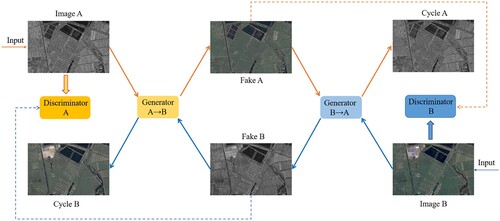
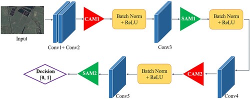
The GANs model mainly includes a generator and a discriminator, which generally uses deep neural networks in practical applications. The generator learns the distribution of the actual image to generate realistic images. The purpose is to deceive the discriminator, and the discriminator needs to judge the authenticity of the received images. With the development of GANs in domain transfer and image generation (Isola et al. 2017), researchers have proposed Cycle GAN (Zhu et al. 2017) with a bidirectional network to achieve efficient transfer. Considering that the cycle consistency of Cycle GAN can improve the efficiency of domain transfer (Luppino et al. 2021; Luppino et al. 2022), Cycle-GANs is used with the attention mechanism as the transfer network of heterogeneous images, and its structure is shown in Figure 1. The entire network is a dual structure, including two generators: Generator (A→B) and Generator (B→A), and two discriminators: Discriminator A and Discriminator B. The model obtains the input Image A from domain A, which is passed to the first generator (A→B). Its task is to transfer a given image from domain A to an image in target domain B. Discriminator B of domain B is used to judge its authenticity. This newly generated image is passed through another generator (B→A), whose task is to transfer the original domain A back to the image Cycle A so that Cycle A is similar to the original input image. This process satisfies the cycle consistency. The entire network is trained continuously until all generators and discriminators reach a dynamic balance; the transformation of heterogeneous images is completed. This model has three main losses: adversarial loss, cyclic consistency loss, and identity loss.

Figure 1. Heterogeneous image transfer network structure.

The adversarial loss is applied to two mapping functions to match the generated image’s distribution with the target domain’s data distribution (Zhu et al. 2017). For the Generator (A→B) and Discriminator B, the target is expressed as: (1) $L_{GAN}(G_{AB},D_B,A,B)={\mathrm{E}}_{y\sim p_{data}\left(y\right)}[\log D_B(y\left)\right]+{\mathrm{E}}_{x\sim p_{data}\left(x\right)}[\log (1-D_B\left(G_{AB}\right(x\left)\right)\left)\right]$(1) Among them $G_{AB}$ is the generator that transforms the image of domain A into the image of domain B, x and y are the input images corresponding to domain A and B, respectively, and $D_B$ aims to distinguish the translation sample $G_{AB}\left(x\right)$ from the real sample y. The training process $G_{AB}$ and $D_B$ compete against one another to minimize this goal, that is $\underset{G_{AB}}{min}\underset{D_B}{max}{L}_{GAN}(G_{AB},D_B,A,B)$. A similar adversarial loss is introduced for the generator and its discriminator that maps from the B to A domain: $\left(\underset{G_{BA}}{min}\underset{D_A}{max}{L}_{GAN}\right(G_{BA},D_A,B,A\left)\right)$.

The adversarial loss alone does not guarantee that the learned function can accurately map the image from domain A to B. The cyclic consistency loss prevents the learned mapping $G_{AB}$ and $G_{BA}$ from contradicting each other. For domain A, the image translation cycle should enable x to remap back to the original image, namely $x$→$G_{AB}\left(x\right)$→$G_{BA}\left(G_{AB}\right(x\left)\right)$≈$x$. Therefore, the cyclic consistency loss is used to incentivize this mapping: (2) $L_{cyc}(G_{AB},G_{BA})={\mathrm{E}}_{x\sim p_{data}\left(x\right)}[\Vert G_{BA}\left(G_{AB}\right(x\left)\right)-x{\Vert }_1]+{\mathrm{E}}_{y\sim p_{data}\left(y\right)}[\Vert G_{AB}\left(G_{BA}\right(y\left)\right)-y{\Vert }_1]$(2) The generator $G_{AB}$ is used to generate the domain B style image. To prevent the change in the tone of the generated image, $G_{AB}\left(y\right)$ and $y$ should be as close as possible. Therefore, the introduction of Identity loss is as follows: (3) $L_{Identity}(G_{AB},G_{BA})={\mathrm{E}}_{x\sim p_{data}\left(x\right)}[\Vert G_{BA}\left(x\right)-x{\Vert }_1]+{\mathrm{E}}_{y\sim p_{data}\left(y\right)}[\Vert G_{AB}\left(y\right)-y{\Vert }_1]$(3) Combining the above losses, the final objective function in this transfer network is: (4) $G_{AB}^{\ast },G_{BA}^{\ast }=\arg \underset{G_{AB},G_{BA}}{min}\underset{D_x,D_y}{max}\left(L_{GAN}\right(G_{AB},D_B,A,B)+\alpha L_{cyc}(G_{AB},G_{BA})+\text{β}{L}_{Identity}(G_{AB},G_{BA}\left)\right)$(4) Among them $\alpha$ and $\text{β}$ are the proportions of the control cycle consistency loss and the identity loss, whose values are 10 and 5, respectively.

3. Methodology

3.1. Details of proposed transformation network

The Transformation Network proposed in this paper has two sub-networks of Generator and Discriminator. A lightweight attention module is added to these two sub-networks, aiming to accelerate the convergence of the model and improve the efficiency of the heterogeneous image domain transfer.

1. Attention module: The attention mechanism refers to a method that pays attention to the important information of the current task while ignoring irrelevant information. In recent years, it has been used widely in various deep learning tasks (Hu 2020; Zeyer et al. 2018; Wang et al. 2020), and it has achieved good results. In the image translation method based on the GAN series, the attention mechanism is introduced to realize the efficient transfer of image style, which has been confirmed in the literature (Chen et al. 2018; Emami et al. 2020; Zhang et al. 2019a). Since our method is unsupervised and has little data, it is difficult to guarantee that the transformation of the entire feature domain is fully realized in Cycle GAN. Therefore, the efficiency of domain transformation is improved by adding an attention module and, at the same time, can accelerate the convergence of the model. Inspired by the work of (Woo et al. 2018), a lightweight attention module is designed from two dimensions, channel, and space. This has been applied to the generator and the discriminator of the above transfer network to achieve more accurate transfer effects. Figure 2 shows the proposed attention module structure used in the transfer network, (a) is the channel attention module, and (b) is the spatial attention module.

Figure 2. The attention module is used in the image transfer network. (a) Channel attention module, (b) Spatial attention module.

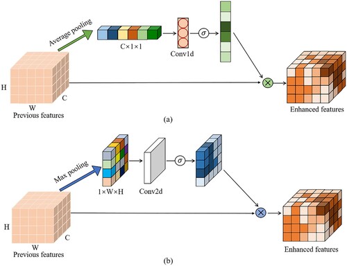
Channel Attention Module (CAM) aims to extract meaningful information from each channel in the feature map. First, each channel in the feature block is averaged and pooled to compress the original feature into a $C\times 1\times 1$ vector. A one-dimensional convolution operation is then applied, followed by the activation function to find the channel weights. The original feature is multiplied by the weight coefficient in the channel dimension to obtain a globally enhanced channel attention feature map (M_C), whose expression is as follows: (5) $M_C=\sigma \left(conv1d\right(Avgpool\left(F\right)\left)\right)\otimes F$(5) where F is the original feature map, $\otimes$represents channel-by-channel multiplication, $\sigma \left(\cdot \right)$is the sigmoid activation function, $conv1d$and$Avgpool$represents one-dimensional convolution and average pooling operations, respectively.

Spatial Attention Module (SAM) aims to extract meaningful information from each pixel in the feature map. First, the spatial elements in each feature block are subjected to maximized pooling on the channel dimension, and the feature block is compressed into a $1\times W\times H$feature map. The spatial weight coefficient is formed using the two-dimensional convolution operation and the activation function. Each position pixel in the original feature is multiplied by the spatial weight coefficient to obtain a locally enhanced spatial attention feature map (M_S), whose expression is as follows: (6) $M_S=\sigma \left(conv2d\right(Maxpool\left(F\right)\left)\right)\otimes F$(6) where$\otimes$represents element multiplication$conv2d$and$Maxpool$represents two-dimensional convolution and maximum pooling operations, respectively.

In the designed CAM and SAM, the average pooling and maximum pooling methods are used to reduce the space and channel dimensions. The two modules obtain the change information after the global and local enhancements. To achieve a better image translation effect, they connect in different ways with the generator and the discriminator.

(B) Generator: The generator is constructed using encoding, transformation, and decoding. The structure of the generator proposed in this paper is shown in Figure 3. First, Features are extracted from the input image (real image) through convolution and downsampling operations, and then the image’s feature vector in the A domain is transferred to the feature vector in the B domain in the attention-based ResNet module. Finally, the deconvolution layer is used for upsampling the feature vector to generate the transferred image (fake image).

Figure 3. The generator’s structure is based on the attention mechanism in the transformation network.

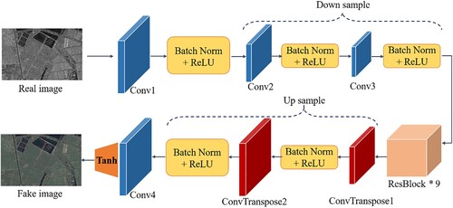
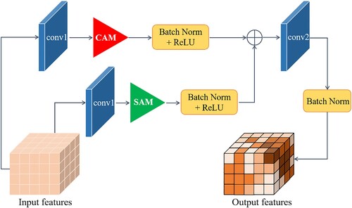
In Figure 3, ‘ResBlock’ is the key module to realize feature transformation. Resblock is the basic unit of the ResNet backbone (He et al. 2016), which is divided into two parts: direct mapping and residual. We add channel and spatial attention to these two places, respectively. Subsequently, two parts are added and sent to the next resblock to perform feature transformation, forming a residual module based on the attention mechanism. Its structure is shown in Figure 4. By fusing the feature maps that have passed through the channel and spatial attention, the global and local information can be taken into account, and the convergence of the generator model can be accelerated while the image transfer is accurately completed. Nine resblocks are connected in series by deepening the number of network layers to extract high-dimensional features and increasing the number of attention modules to enhance useful information and suppress irrelevant information.

Figure 4. Resblock structure based on attention mechanism.

(C) Discriminator: The role of the discriminator is to take an image as input and predict whether it is the original image (Real image) or the output image (Fake image) of the generator. Figure 5 shows the proposed discriminator network based on the attention mechanism, which extracts features from the input image through a simple convolutional neural network to determine whether the image belongs to the specific category (real image or fake image). The essence of a discriminator is a binary classifier, in which an attention mechanism is added to improve the classification accuracy.

Figure 5. Discriminator structure based on attention mechanism in transformation network.

3.2. CD framework for transformed images

In the transformation network proposed in this paper, two heterogeneous images are transformed from a lower-dimensional feature domain to a higher-dimensional feature domain and then obtain the changed regions in the high-dimensional feature space. Since the high-dimensional feature domain contains additional information, it is helpful to detect more changed features, so the high-dimensional feature domain in the heterogeneous image pair is selected as the common domain for subsequent change detection.

Although the above transfer network can transform heterogeneous images into similar feature domains, their pixel differences may still be significant, and unnecessary noise will be introduced during the transformation process. Therefore, a three-step post-processing algorithm is proposed to obtain an accurate heterogeneous change map.

1. Calculate the difference map: According to the channel dimension, we calculate the Euclidean distance of the corresponding spatial position from the image transferred to domain B (Generate image) and the real image of domain B (Image B). And then, the maximum distance in each channel is taken as the difference values of spatial pixels to generate a single-channel difference map.

2. Threshold segmentation: Determine the segmentation threshold of pixel intensity, and only retain the pixels with intensity higher than the threshold in the difference map, and convert the difference map into a binary change map. The maximum between-class variance method (OTSU) (Otsu 1979) is primarily used to determine the threshold value. It divides the image into two parts: background and foreground, according to the grayscale characteristics of the image. Variance is a measure of the uniformity of gray distribution. The larger the inter-class variance between the background and the foreground, the greater the difference between the two parts of the image. So the segmentation with a large inter-class variance indicates a low probability of misclassification. OTSU is computationally simple, not affected by image brightness and contrast, and does not require additional parameters compared with other segmentation methods. This method has been proven to have excellent segmentation effects in literatures (Luppino et al. 2022; Luppino et al. 2022).

3. Reduce false detection noise: Since the change area of interest in CD tasks is usually large, we filter out high-frequency noise to remove isolated small points in the binary change map to generate a more accurate final change map. A Discrete Cosine Transform (DCT)-based filter is used to remove the false detection noise from the binary change map. The DCT-based filtering method has a good noise suppression effect in the homogeneous area of the image and can retain the edges and detailed features (Ning and Ke 2012). Moreover, the calculation speed of the DCT transform is fast. Therefore, for image noise filtering with unknown noise-related parameters and non-stationary conditions, the adaptive denoising technology of the DCT transform can get excellent results.

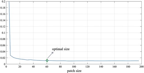
DCT is a special form of Discrete Fourier Transform (DFT) (Oktem and Ponomarenko 2007). If in the Fourier series expansion, the function to be expanded is a real even function, then only the cosine term is included in the Fourier series, and thus the DCT transform can be obtained. After DCT, the binary change map forms the DCT coefficient map. The upper left corner represents the low-frequency part. The farther away from the upper left corner, the higher the frequency. The position where the more prominent value component appears represents the frequency distribution of the image. A patch proportional to the image size is used to intercept the low-frequency part of the DCT coefficients to filter out high-frequency noise. For the size of the image patch, a series of reference values are set. According to experiments, it is found that the smaller the size of the selected image patch, the more pronounced the noise removal, but the more the loss in the details of the changed image. The larger the selected image patch, the more details of the changed image are retained, but the noise removal effect is poor. Therefore, the image patch size has become an important factor in the quality of the generated change map.

In order to select the appropriate image patch size, an adaptive method is proposed based on the pixel intensity ratio to determine this parameter, i.e. the initial patch size is 1/100 of the original image, and the proportion of white pixels in the patch is calculated and recorded. The patch size is then expanded outwards in units of five pixels. The above steps are repeated for each expansion, and the proportion of white pixels in the patch is recorded until the patch size reaches half of the original image. During this process, the aspect ratio of the patch is always consistent with the original image. Finally, the value obtained by each expansion is plotted, as shown in Figure 6. The abscissa represents the size of the patch, and the ordinate represents the proportion of white pixels in the patch. It can be seen that when the patch is small, the white pixels account for more, and the change is drastic. As the patch size increases, the proportion decreases and tends to stabilize. The point marked in Figure 6 is where the polyline begins to flatten. Before this, the proportion of low-frequency information in the image decreases before becoming constant. The expansion of the patch size did not add new meaningful low-frequency information; instead, high-frequency noise was introduced. Therefore, the patch size corresponding to the point where the slope of the broken line tends to stabilize is considered the optimal value for restoring the low-frequency part of the image. Finally, the DCT coefficients in the window are retained, and the others are set to zero, and then the DCT inverse transformation is performed to obtain the change map for removing high-frequency noise (false detection noise).

Figure 6. Line chart of pixel intensity ratio in the patch.

The above-mentioned heterogeneous CD post-processing algorithm is summarized in Algorithm 1, A, and B, respectively represent the spatial domain of the heterogeneous bi-temporal image, W, H, C are the length, width, and channel number of the image, respectively, the patch is the image block determined according to the DCT coefficient.

Table

Algorithm 1 Post-processing

1 Compute $DI=\Vert G_{AB}\left(x\right)-y{\Vert }_1$, $x\subset A,y\subset B$

for all pixels $(x,y)\in \left\{\right(1,2,\cdots ,W),(1,2,\cdots ,H\left)\right\}$

for all channels $c\in \{1,2,\cdots ,C\}$, do

Compute $D{I}^{\mathrm{\prime }}(x,y)=max\left[DI\right(x,y,c\left)\right]$

end for

end for

2. Compute $T=OTSU\left(D{I}^{\mathrm{\prime }}\right)$

for all pixels $(x,y)$ in $D{I}^{\mathrm{\prime }}$, do

$D{I}^{\mathrm{\prime }}(x,y)=\left\{\begin{array}{c}1,\begin{array}{c}\end{array}D{I}^{\mathrm{\prime }}(x,y)\ge T\\ 0,\begin{array}{c}\end{array}D{I}^{\mathrm{\prime }}(x,y)<T\end{array}\right\}$

3. Compute $CM=DCT\left(D{I}^{\mathrm{\prime }}\right)$

Compute $C{M}^{\mathrm{\prime }}(x,y)=\left\{\begin{array}{c}C{M}^{\mathrm{\prime }}(x,y),\begin{array}{c}\end{array}(x,y)\subseteq patch\\ 0,\begin{array}{c}\end{array}\begin{array}{c}\end{array}\begin{array}{c}\end{array}\begin{array}{c}\end{array}\begin{array}{c}\end{array}\begin{array}{c}\end{array}\begin{array}{c}\end{array}(x,y)\not\subset patch\end{array}\right\}$

Compute $CM=iDCT\left(C{M}^{\mathrm{\prime }}\right)$

4. Experiments

In this section, the effectiveness of the proposed method is verified using three groups of typical datasets with bi-temporal heterogeneous images. 4.1 Section introduces the experimental details. 4.2 Section introduces the bi-temporal heterogeneous dataset used in this paper for remote sensing CD. 4.3 Section introduces several excellent heterogeneous CD methods and the related evaluation metrics. A comprehensive comparative analysis of the experimental results is shown in Section 4.4, and Section 4.5 conducts the ablation studies.

4.1. Implementation details

The proposed domain transformation network is trained and tested on a server powered by a Titan RTX GPU and an Intel(R) Xeon(R) W-2245 CPU (3.9 GHz, 256GB RAM). In order to reduce the computational pressure, the entire image is cropped into small-sized patches as the input of the network. 32×32, 64×64, 128×128, and 256×256 patches were used for training, and the optimal patch size was obtained according to the experimental results. We use the Pytorch deep learning framework with batch size set to 16, and training epochs set to 200. The training process uses a stochastic gradient descent (SGD) algorithm with momentum set to 0.99 and weight decay to 0.0005 to optimize the model. The initial learning rate is 0.01, and the learning rate decreases linearly as the number of iterations increases.

4.2. Datasets introduction

The CD experiments are conducted on three heterogeneous datasets, among which the California dataset is an actual case of heterogeneous CD for emergency situations. It is not easy to obtain short-term heterogeneous bi-temporal images in public datasets, so we use the proposed method to conduct experiments on two heterogeneous datasets with a long interval, Shuguang and Toulouse. It is found that the proposed method achieves excellent CD results (Section 4.4). In addition, before the CD of heterogeneous images, the co-registration of images is an indispensable work. The publisher has co-registered all datasets in this section, and the proposed method directly performs CD experiments on the registered bi-temporal heterogeneous images.

1. California dataset: Figure 7 shows the heterogeneous remote sensing images before and after the floods in the area near California, between January to February 2017. (a) is a multi-spectral image collected by Landsat 8 before the flood, including 11 spectral bands from dark blue to thermal infrared. (b) is a SAR image collected by Sentinel-1A after the flood. The three channels are polarization VV, VH, and the ratio between the two intensities. (a) and (b) are all pseudocolor images for the convenience of visualization. The two temporal images have undergone preprocessing, including resampling, registration, and cropping. Both the images are 3500 × 2000 pixels with a spatial resolution of 30 meters. (c) is the Ground truth map provided by Luppino et al. (2019).

2. Shuguang dataset: Figure 8 shows the bi-temporal heterogeneous remote sensing image of Shuguang Village, Dongying City, China, (a) is the SAR image taken by the RADARSAT-2 satellite in June 2008, (b) is the optical image of the same area taken by the Quick bird satellite in September 2012, (c) is the Ground truth map of the changing situation. The images in two temporal are registered, and both are 593×921 pixels, with a spatial resolution of 8 meters. This pair was obtained from Liu et al. (2018).

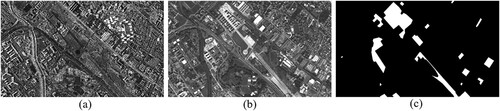
3. Toulouse dataset: Figure 9 shows the bi-temporal heterogeneous remote sensing image of Toulouse, France, (a) is the SAR image taken by TerraSAR-X satellite in February 2009, (b) is the optical panchromatic image taken by Pleiades satellite in July 2013. (c) is the Ground truth map of the changing situation. Two of the temporal images were registered to 4404 × 2604 pixels, and the SAR images were resampled and registered by Prendes (2015) using optical imagery with a spatial resolution of 2 m.

Figure 7. California dataset. (a) Landsat 8 image at time T1, (b) Sentinel-1A image at time T2, (c) Ground truth map.

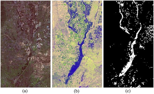
Figure 8. Shuguang dataset. (a) SAR image at time T1, (b) optical image at time T2, (c) Ground truth map.

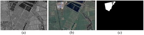
Figure 9. Toulouse dataset. (a) SAR image at time T1, (b) optical panchromatic image at time T2, (c) Ground truth map.

4.3. Benchmark methods and evaluation metrics

In order to evaluate the effectiveness of the proposed method, we use the following benchmark methods to perform heterogeneous CD and compare their performance on the above four datasets:

1. CVA (change vector analysis) (Johnson and Kasischke 1998): A classic method for pre-classification CD. The magnitude of the change is indicated by the magnitude of the vector between the two temporals, and the threshold for the separation determines the area of change/unchanged between the two temporals.

2. SCCN (symmetric convolutional coupling network) (Liu et al. 2018): An unsupervised deep convolution coupling network for heterogeneous image CD. The symmetric network is trained to transform two images into a common feature space. The bi-temporal feature maps are directly compared in this feature space, and the final change map is obtained according to the threshold algorithm.

3. NPSG (nonlocal patch similarity-based graph) (Sun et al. 2021): A new CD method based on the similarity measurement between heterogeneous images. First, a map is constructed for each patch based on the similarity of nonlocal patches to establish the connection between heterogeneous data, and then the change area is detected by measuring the degree of conformity between the map structures of the two images.

4. INLPG (improved nonlocal patch-based graph) (Sun et al. 2022): A CD method based on structural consistency. This method detects changes by comparing the structure of the two images instead of comparing the pixel values of the images. The structural comparison is achieved by constructing and mapping an improved nonlocal patch-based map (NLPG).

5. CAA (code-aligned autoencoders) (Luppino et al. 2022): A heterogeneous CD method based on affinity matrix alignment code space. Extracting the pixel relationship information captured at the input using the field-specific affinity matrix forces the code space’s alignment and reduces the impact of changing pixels on the learning target.

Four evaluation metrics are used to evaluate the performance of the proposed CD method, namely Precision (Pr), Recall (Re), F1 score (F1 Score), and Kappa coefficient (Kappa). In the CD task, the Pr indicates the accuracy of detecting the changed pixels, and the Re indicates the completeness of the changed pixels detected by the model. They use true positives (TP), true negatives (TN), false positives (FP), and false negatives (FN) to describe. F1 Score and Kappa reflect the model’s overall performance, and a more significant value reflects the better performance of the model. The four evaluation metrics are described as: (7) $Pr={\displaystyle \frac{TP}{TP+FP}}$(7) (8) $Re={\displaystyle \frac{TP}{TP+FN}}$(8) (9) $\frac{{\displaystyle F1Score=2Pr\times Re}}{Pr+Re}$(9) (10) $Kappa={\displaystyle \frac{P_o-P_e}{1-P_e}}$(10)

Among them, the Kappa calculation formula $P_o$represents the overall accuracy (OA), $P_e$represents the ratio of expected consistency between the true value and the predicted value under a given category distribution (El Amin, Liu, and Wang 2017). The expression of $P_o$ and $P_e$ is as follows, where N is the total number of image pixels. (11) $P_o={\displaystyle \frac{TP+TN}{N}}$(11) (12) $P_e={\displaystyle \frac{(TP+FP)(TP+FN)+(FN+TN)(FP+TN)}{N^2}}$(12)

4.4. Comparison of experimental results

4.4.1. Experiments on California dataset

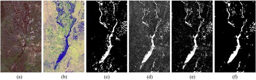
Figure 10 shows the CD process of our method on the California dataset, where (a), (b), and (c) are T1 image, T2 image, and Ground truth map, respectively. After passing through an image transfer network based on the attention mechanism, the Euclidean distance of the corresponding pixel space between the transferred image and the original image is found, and it is converted into a single-channel difference map as shown in Figure 10 (d). (e) is the binary change map after OTSU threshold segmentation, (f) is the final change map after DCT noise reduction. Compared to figure (e), the final change figure (f) has significantly reduced false detection pixels, reduced noise, and can more accurately detect the change area of the SAR and multi-spectral bi-temporal images.

Figure 10. The CD process of the proposed method on dataset 1 (California). (a) Landsat 8 image at time T1, (b) Sentinel-1A image at time T2, (c) Ground truth map, (d) difference map, (e) binary change map, (f) final change map after DCT noise reduction.

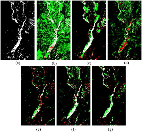
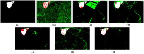
Figure 11 shows the CD results obtained by different methods on the California dataset, (a) is the Ground truth map, (b)-(g) are the change maps obtained by CVA, SCCN, NPSG, INLPG, CAA, and the method proposed in this paper, respectively. A comparison shows that CVA (Figure 11 (b)) has the worst results, barely able to handle the noise from spurious changes. The results of SCCN (Figure 11 (c)) can correctly detect a large-area change, but there are both false and missed detections for small changes. NPSG (Figure 11 (d)) failed to detect the shape of the change area, missed large area change pixels, and has incorrectly detected the subtle background pixels as changed pixels. INLPG (Figure 11 (e)) significantly reduces the number of incorrect detections but still does not detect a few small areas of change. CAA (Figure 11 (f)) and the proposed method (Figure 11 (g)) are similar, and both can detect large areas of change covered by floods, but it is difficult to detect smaller flood areas correctly. The difference is that using the proposed method, the boundary of the change area is more compact, but it merges closely located small change areas into a connected domain, resulting in more incorrectly detected pixels.

Figure 11. The CD results of different methods on dataset 1 (California). (a) Ground truth map. Change maps produced by (b) CVA, (c) SCCN, (d) NPSG, (e) INLPG, (f) CAA and (g) Proposed method. In the figure, Black: TN; White: TP; Green: FP; Red: FN.

In order to quantitatively evaluate the performance of the detection results of the above methods, Table 1 shows the evaluation metrics of the experimental results obtained by different methods on the California dataset. The proposed method achieves the best detection performance with the highest Re (0.7231), F1 Score (0.6099), and Kappa (0.5764). Similarly, the deep learning-based methods, SCCN, CAA, and the proposed method perform better on the California dataset than NPSG and INLPG. This shows that for multi-spectral heterogeneous images with a large amount of data, deep learning networks for CD are more competitive. Compared to the suboptimal methods CAA and SCCN, the F1 Score metric of the proposed method has increased by 1.41% and 4.57%, respectively, and the Kappa has increased by 1.06% and 6.04%, respectively. However, for the Pr metric, the proposed method is 0.17% lower than the CAA. This is because some falsely detected pixels caused by the small filter window in the adaptive DCT algorithm are not filtered out, but the Re metric of the proposed method is significantly improved, reflecting the comprehensive metrics F1-Score and Kappa make up for the lack of Pr decline to a certain extent. The CVA method takes the least CD time in terms of computation time, while the INLPG method takes the longest, and the three deep learning-based CD methods, SCCN, CAA, and the proposed method, require similar time (including the sum of training and testing time).

Table 1. Quantitative results of different methods on dataset 1 (California).

Different methods	Pr	Re	F1-Score	Kappa	Time (s)
CVA	0.2428	0.1540	0.1885	0.1194	4.92
SCCN	0.4729	0.6992	0.5642	0.5160	952.18
NPSG	0.4173	0.1408	0.2106	0.1554	6.93
INLPG	0.4359	0.4189	0.4272	0.4004	3981.94
CAA	0.5291	0.6818	0.5958	0.5658	838.52
Proposed method	0.5274	0.7231	0.6099	0.5764	1017.60

4.4.2. Experiments on Shuguang dataset

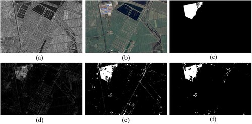
Figure 12 shows the CD process of the proposed method on the Shuguang dataset, where (a) and (b) are the SAR and visible optical image, respectively, (c) is the Ground truth map, (d) is the difference map obtained after the transfer network, (e) (f) are the change maps obtained after the post-processing steps proposed in this paper.

Figure 12. The CD process of the proposed method on dataset 2 (Shuguang). (a) SAR image at time T1, (b) optical image at time T2, (c) Ground truth map, (d) difference map, (e) binary change map, (f) final change map after DCT noise reduction.

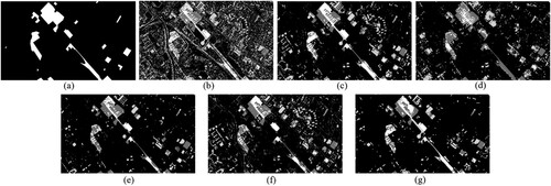
Figure 13 shows the CD results obtained using different methods on the Shuguang dataset, (a) is the Ground truth map, (b)-(g) are the change maps obtained by CVA, SCCN, NPSG, INLPG, CAA and proposed in this paper, respectively. In the change map, black represents TN, white represents TP, green represents FP, and red represents FN. This comparison shows that CVA (Figure 13 (b)) has the most false and missed pixels. SCCN (Figure 13 (c)) has a high false detection rate, and some pixels are missed. NPSG (Figure 13 (d)) has the least missed pixels and has a higher recall rate, but the false detection rate is high. INLPG (Figure 13 (e)) has fewer false detection pixels, but it misses many real change pixels, missing the shape of the change area, and the change from farmland to building cannot be recognized properly. CAA can detect the boundary of the changed area (Figure 13 (f)), but many unchanged pixels are misidentified, and it lacks effective post-processing steps to remove the misdetection noise of some details. The proposed method (Figure 13 (g)) has fewer missed pixels and fewer false detections for changing pixels, and the obtained change area has a complete boundary and compact interior. The consistency of the change map and the ground truth map is optimal in the above method.

Figure 13. The CD results of different methods on dataset 2 (Shuguang). (a) Ground truth map. Change maps produced by (b)CVA, (c) SCCN, (d) NPSG, (e) INLPG, (f) CAA and (g) Proposed method.

In order to quantitatively evaluate the performance of the detection results of the above methods, Table 2 shows the evaluation metrics of the experimental results obtained by different methods on the Shuguang dataset. The proposed method achieves the best detection performance with the highest Pr (0.8115), F1 Score (0.8314), and Kappa (0.8241). NPSG has the highest Re (0.9297), but its Pr is significantly lower, decreasing overall performance. Due to insufficient network fitting, the methods based on deep learning, SCCN, and CAA result in poor image transform effect, and they lack effective post-processing steps, resulting in poor performance of these two methods. Compared with the sub-optimal method INLPG, the proposed method achieved 9.02% and 9.35% improvements on the comprehensive metrics F1 Score and Kappa, respectively. From Table 2, CVA and NPSG methods are computationally faster, the CAA method is the slowest, and the computational complexity of SCCN, CAA, and the proposed method are approximately the same.

Table 2. Quantitative results of different methods on dataset 2 (Shuguang).

Different methods	Pr	Re	F1-Score	Kappa	Time (s)
CVA	0.1048	0.6365	0.1800	0.1183	2.16
SCCN	0.2940	0.8760	0.4402	0.4015	403.71
NPSG	0.4944	0.9297	0.6455	0.6256	3.97
INLPG	0.7641	0.7196	0.7412	0.7306	199.02
CAA	0.4347	0.8831	0.5826	0.5585	412.53
Proposed method	0.8115	0.8523	0.8314	0.8241	387.65

4.4.3. Experiments on Toulouse dataset

Figure 14 shows the CD process of the proposed method on the Toulouse dataset, where (a) and (b) are the SAR, and optical panchromatic image, respectively, and (c) is the Ground truth map, (d) is the difference map obtained after the transfer network, (e) (f) are the change maps obtained after the post-processing steps proposed in this paper.

Figure 14. The CD process of the proposed method on dataset 3 (Toulouse). (a) SAR image at time T1, (b) optical panchromatic image at time T2, (c) Ground truth map, (d) difference map, (e) binary change map, (f) final change map after DCT noise reduction.

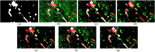
Figure 15 shows the CD results obtained by different methods on the Toulouse dataset, (a) is the Ground truth map, (b)-(g) are the change maps obtained by CVA, SCCN, NPSG, INLPG, CAA, and the proposed method, respectively. The changing targets in the Toulouse dataset are mainly buildings and roads. Since both SAR and panchromatic images are single-band images, the spectral information is not rich enough, so the CD on the Toulouse dataset is challenging. By comparison, it can be seen that the change map generated by the proposed method has the least number of falsely detected pixels and significantly removes the high-frequency noise from the image. In terms of detection integrity, the proposed method almost completely detects the small changes in the road (below Figure 15 (f)), while other benchmark methods miss this detail. In addition, the proposed method has a higher recall rate for the change areas with many buildings, as in the upper left of the image, which is significantly higher than that of CVA (Figure 15 (b)), NPSG (Figure 15 (d)), INLPG (Figure 15 (e)), and CAA (Figure 15 (f)), while SCCN (Figure 15 (c)) has significantly higher false-detection pixels in other regions than the proposed method. Due to the small filter window of the adaptive DCT denoising algorithm in the Toulouse experiment, some small change areas are not detected in the obtained change map.

Figure 15. The CD results of different methods on the dataset 3 (Toulouse). (a) Ground truth map. Change maps produced by (b) CVA, (c) SCCN, (d) NPSG, (e) INLPG, (f) CAA and (g) Proposed method. In the figure, Black: TN; White: TP; Green: FP; Red: FN.

In order to quantitatively evaluate the performance of the above methods, Table 3 shows the evaluation metrics of the experimental results obtained by different methods on the Toulouse dataset. The proposed method achieved the best results in all four evaluation metrics compared to other benchmarks. Compared with the suboptimal method SCNN, F1-Score and Kappa are improved by 3.26% and 6.52%, respectively. It can be seen that the proposed method can also achieve competitive detection results on the challenging dataset Toulouse. Facing the Toulouse dataset with a larger size, the CD time of both NPSG and INLPG exceeds 50 min, while the proposed method’s total training and testing time are about 15 min.

Table 3. Quantitative results of different methods on dataset 3 (Toulouse).

Different methods	Pr	Re	F1 Score	Kappa	Time (s)
CVA	0.1428	0.5367	0.2256	0.1142	7.54
SCCN	0.3359	0.5085	0.4071	0.3370	962.17
NPSG	0.3058	0.2290	0.2618	0.1879	3371.42
INLPG	0.3391	0.3962	0.3654	0.3151	4696.05
CAA	0.2526	0.4048	0.3111	0.2327	568.93
Proposed method	0.3621	0.5597	0.4397	0.4023	908.76

4.5. Ablation studies

4.5.1. Parameter analysis

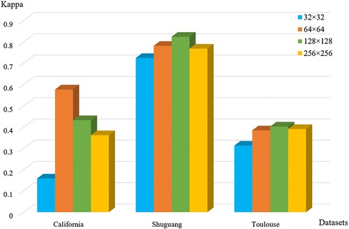
In the proposed transfer network for heterogeneous images, the difference in the size of the input image patch will lead to the difference in the transfer effect. Therefore, for different datasets, image patches of different sizes are used to train the transfer network to determine the size of the image patch by testing the final CD effect. Four patches of sizes 32×32, 64×64, 128×128, and 256×256 are used for training, respectively. The final CD metric Kappa obtained on the three datasets is shown in Figure 16. It is found that training the network using a 64×64 patch on the California dataset gives the best results. 128×128 patch on the Shuguang dataset gives the best results. Similarly, using the 128×128 patch on the Shuguang and Toulouse dataset gives the best results. By analyzing the change details of the original dataset, it is considered that the size of the patch selected is related to the area and concentration of the change part. The Shuguang dataset has only one change part, the change area is relatively large, and the overall image is small (593×921). Similarly, the Toulouse dataset has relatively regular change areas, and the size of the whole image and the changed areas are larger. Therefore, both use 128×128 patches to capture multiple change details to achieve a complete CD map. The California dataset has the most scattered change part, a relatively small area, making the CD task difficult, so the 64×64 patch is most suitable.

Figure 16. Comparison results of CD metric Kappa obtained using different patch training networks.

In our method, the difference map of the transferred image must be a single channel to form a binary change map, which requires converting the multi-channel difference map into a single channel. Usually, the reduction of channel dimensions uses simple methods, such as the maximum, the minimum, and the average value of each channel. In order to determine which method to use, the effect of the change map was obtained by each dimensionality reduction method on four datasets. The comprehensive metrics F1 Score and Kappa are shown in Table 4. Through comparison, it was found that the effect of the change map obtained by the maximum sampling method is the best of the three datasets. The large Euclidean distance between two images indicates that the pixel is likely to change, and the accuracy of the CD is ensured by taking the maximum value in the channel. The corresponding pixels will be very different, especially in heterogeneous CD, regardless of whether it is changed or not. If the minimum sampling is selected, many incorrectly detected pixels will be added. Therefore, the change map obtained using the maximum sampling has a more competitive effect.

Table 4. Comparison of different dimensionality reduction methods for the difference map on the three datasets.

Datasets	Average sampling		Minimum sampling		Maximum sampling
	F1-Score	Kappa	F1-Score	Kappa	F1-Score	Kappa
California	0.3186	0.2853	0.3940	0.3647	0.6099	0.5764
Shuguang	0.6683	0.6446	0.5687	0.5372	0.8314	0.8241
Toulouse	0.3998	0.3679	0.4020	0.3891	0.4397	0.4023

4.5.2. Effect of adaptive DCT

The DCT denoising algorithm is improved in the post-processing step of heterogeneous CD, enabling it to adaptively determine filtering parameters according to the difference map properties. The CD results are compared with other classical denoising methods (original DCT, Gaussian filtering, Mean filtering, Wavelet transform) and Morphological filtering (Open and Close operations) on three datasets to verify the effectiveness of the adaptive DCT method. The F1-Score and Kappa metrics obtained from the CD experiment are shown in Table 5. Since it takes many experiments to determine the optimal parameters of each algorithm, in order to reduce the time cost, we set the parameters in these four denoising methods empirically. By comparison, it can be found that the proposed adaptive DCT method is excellent in removing pseudo-change pixels and obtaining a change map that is closer to the Ground Truth. Since the parameters of other algorithms are determined by empirical values, it means that the denoising performance may not be optimal. However, in practical applications, it is expected to perform CD automatically and quickly, and accurately, instead of consuming much time by manually adjusting parameters. In addition, it was noticed that the F1-Score obtained by Adaptive DCT in the California dataset is not as good as that of the Open operation method. This is because some small change areas in the California dataset make Adaptive DCT misjudge it as noise and filter it, resulting in low Recall of the generated change map. In future research, the proposed algorithm will be improved to detect small changed regions.

Table 5. Comparative experimental results of the proposed adaptive DCT denoising method with other denoising methods.

Denoising methods		F1-Score / Kappa (%)
		California	Shuguang	Toulouse
Filter denoising	DCT	56.77 / 54.38	82.37 / 81.86	38.62 / 34.97
	Gaussian filter	55.29 / 53.41	77.94 / 75.24	41.35 / 38.62
	Mean filter	51.08 / 47.10	78.35 / 79.69	35.94 / 30.50
	Wavelet transform	57.49 / 55.75	82.04 / 81.70	40.09 / 38.28
Morphological denoising	Open operation	61.22 / 57.58	81.26 / 78.41	37.96 / 35.17
	Close operation	54.88 / 50.27	82.24 / 80.29	32.88 / 29.43
Proposed	Adaptive DCT	60.99 / 57.64	83.14 / 82.41	43.97 / 40.23

4.5.3. Effects of attention and post-processing algorithm

This paper has two main contributions: one is to propose an image transfer network based on the attention mechanism, and the other is to design a post-processing algorithm for CD based on adaptive DCT. In order to verify the role of the proposed attention module and post-processing algorithm in the detection of heterogeneous changes, an ablation experiment is carried out in this section.

Different models are considered with and without the attention module and the post-processing algorithm. These models are trained and tested using the three datasets. Furthermore, the Kappa metric is calculated for each model, as shown in Table 6. It can be seen that after adding the attention module and post-processing algorithm, the CD performance of the model has been significantly improved. In addition to the Shuguang dataset, the post-processing algorithm contributes slightly more to improving the model performance than the attention module. This means that the proposed post-processing step of heterogeneous CD is important to improve detection accuracy. The introduction of the attention module makes the domain transfer network pay more attention to the essential features of images, ensuring the reliability of domain transfer between heterogeneous images. Therefore, the attention mechanism and the DCT noise reduction algorithm, proposed in this paper jointly improve the model’s performance in detecting changes with heterogeneous images at the domain transfer and post-processing aspects and make the model more robust.

Table 6. Ablation experiment results of attention module and post-processing algorithm. The Kappa metric is reported.

Attention module	Post-processing Algorithm	Datasets
		California	Shuguang	Toulouse
×	×	0.4265	0.5896	0.2317
√	×	0.4328	0.7623	0.3079
×	√	0.4837	0.7594	0.3268
√	√	0.5764	0.8241	0.4023

5. Discussion

In this Section, we discuss the experimental results of the proposed method on the above three datasets. It mainly includes CD performance on heterogeneous images with different spatial resolutions and different spectrum, and the relationship between CD effect and time cost. Table 7 shows the spatial resolution of the three datasets and the spectral numbers of the corresponding optical images and the performance metrics of the proposed method on these three datasets.

Table 7. The relationship between the proposed method’s CD results and the datasets’ characteristics.

Datasets	Spatial resolution	Spectral number	Time cost	F1 Score	Kappa
Dataset 1(California)	30 m	11	1017.60 s	0.6099	0.5764
Dataset 2 (Shuguang)	8 m	3	387.65 s	0.8314	0.8241
Dataset 3 (Toulouse)	2 m	1	908.76 s	0.4397	0.4023

CD performance at different spatial resolutions. The spatial resolutions of the three heterogeneous datasets selected in this paper after registration are 30, 8 and 2 m, respectively. Combined with the Kappa metric in Tables 1–3, it is found that the proposed method has more advantages than other methods on the datasets with 8 and 2 m resolution. The Kappa of the proposed method in dataset 1 (30 m resolution) is 1.06% higher than that of the suboptimal method, while the Kappa in dataset 2 (8 m resolution) and dataset 3 (2 m resolution) outperforms the suboptimal method by 9.35% and 6.53%, respectively. This is because in the process of domain transformation, higher spatial resolution provides the transformation network with rich ground object information, which improves the efficiency of spatial domain transformation. Therefore, our method is more competitive for CD in medium to high resolution heterogeneous images.

CD performance of different spectral features. In the three heterogeneous datasets, the spectral numbers of the optical images were 11 (multi-spectral), 3 (RGB), and 1 (panchromatic). According to the experimental results, it is found that our method performs well in the dataset 2 with the three bands spectrum. Generally speaking, spatial resolution and spectral resolution are mutually restricted, and the method in this paper can achieve optimal CD results when the two tend to balance. In addition, it can be seen from the reference change map of the three datasets that the shape of the change area in dataset 2 is the most regular, and the distribution of the change pixels in the other two datasets is more scattered, so our method conforms to the subjective judgment of the change area by humans. That is, the dataset 2 with the simplest change distribution has the best CD performance.

The relationship between CD effect and time cost. The time cost of the proposed method on the three datasets is 1017.60s, 387.65s, and 908.76s, respectively. Combined with the time cost of other methods in Tables 1–3, we find that the proposed method’s time cost is generally higher. Except for dataset 2, our method’s time cost is higher than the CAA method, but the F1 Score and Kappa are the best on the three datasets. Compared with the CAA method, the proposed method adds a series of post-processing steps, among which the process of dimensionality reduction and denoising will reduce the speed of the algorithm to a certain extent, so we believe that it is reasonable to trade a small amount of time cost for the improved accuracy of CD results.

6. Conclusions

This work mainly studies the CD of bi-temporal heterogeneous remote sensing images. Due to the different imaging mechanisms of heterogeneous data, the image features are not in the same feature domain. So it is difficult to detect the changes between two temporally heterogeneous images through direct comparison. An unsupervised method was proposed for heterogeneous CD based on Cycle-GANs image transfer network. First, by introducing an attention mechanism, the domain transfer effect of Cycle-GANs is improved so that heterogeneous images can be compared in the same feature domain. Secondly, a post-processing algorithm is designed, and the final change map is obtained through the steps of dimensionality reduction of the difference map, threshold segmentation, and adaptive DCT noise reduction method. Experimental verification was performed on three different types of heterogeneous image datasets, and competitive detection results were obtained. This means that the proposed method can effectively detect the change information of optical and SAR heterogeneous images. Comparing current SOTA algorithms, it is found that the proposed heterogeneous CD method has higher accuracy and stronger robustness. Finally, the optimal patch size of the training transfer network and the dimensionality reduction way of the difference map are obtained through parameter analysis. In the ablation experiments, we further verified the denoising effectiveness of the proposed adaptive DCT and the effectiveness of the attention module and post-processing algorithm. In the future work, we will focus on reducing the time cost of the algorithm, and study the CD method more suitable for medium and low resolution heterogeneous images, and further improve the efficiency of heterogeneous CD.

Acknowledgment

This study is supported by Military Commission Science and Technology Committee Leading Fund of China, grant number 18-163-00-TS-004-080-01.

We would like to express our gratitude to EditSprings (https://www.editsprings.com/) for the expert linguistic services provided.

Disclosure statement

No potential conflict of interest was reported by the author(s).

Data Availability Statement

The datasets used during the current study are available in website (https://www.jianguoyun.com/p/DSJQW_EQ0uCBChjwgZoE).

Additional information

Funding

This work was supported by Military Commission Science and Technology Committee Leading Fund of China: [Grant Number 18-163-00-TS-004-080-01].

References

- Chen, H., and Z. Shi. 2020. “A Spatial-Temporal Attention-Based Method and a new Dataset for Remote Sensing Image Change Detection.” Remote Sensing 12 (10): 1662 (pp. 1–23). doi:10.3390/rs12101662.
- Chen, X., C. Xu, X. Yang, and D. Tao. 2018. “Attention-gan for Object Transfiguration in Wild Images.” In Proceedings of the European Conference on Computer Vision (ECCV), 164–180. doi:10.1007/978-3-030-01216-8_11.
- Daudt, R. C., B. Le Saux, and A. Boulch. 2018. “Fully Convolutional Siamese Networks for Change Detection.” 25t. H IEEE International Conference on Image Processing (ICIP). pp. 4063-4067. doi:10.1109/icip.2018.8451652.
- Doersch, C. 2016. “Tutorial on variational autoencoders.” arXiv preprint arXiv:1606.05908.
- El Amin, A. M., Q. Liu, and Y. Wang. 2017. “Zoom out CNNs Features for Optical Remote Sensing Change Detection.” 2nd International conference on image, vision and computing (ICIVC). (pp. 812-817). doi:10.1109/icivc.2017.7984667.
- Emami, H., M. M. Aliabadi, M. Dong, and R. B. Chinnam. 2021. “Spa-gan: Spatial Attention gan for Image-to-Image Translation.” IEEE Transactions on Multimedia 23: 391–401. doi:10.1109/TMM.2020.2975961.
- Gong, M., X. Niu, T. Zhan, and M. Zhang. 2019. “A Coupling Translation Network for Change Detection in Heterogeneous Images.” International Journal of Remote Sensing 40 (9): 3647–3672. doi:10.1080/01431161.2018.1547934.
- Gong, M., J. Zhao, J. Liu, Q. Miao, and L. Jiao. 2016. “Change Detection in Synthetic Aperture Radar Images Based on Deep Neural Networks.” IEEE Transactions on Neural Networks and Learning Systems 27 (1): 125–138. doi:10.1109/TNNLS.2015.2435783.
- Goodfellow, I., J. Pouget-Abadie, M. Mirza, B. Xu, D. Warde-Farley, S. Ozair, … Y. Bengio. 2014. “Generative Adversarial Nets.” Advances in Neural Information Processing Systems 27: 1–9.
- He, K., X. Zhang, S. Ren, and J. Sun. 2016. “Deep Residual Learning for Image Recognition.” Proceedings of the IEEE Conference on Computer Vision and Pattern Recognition, 770–778. ). doi: 10.1109/cvpr.2016.90
- Hedhli, I., G. Moser, J. Zerubia, and S. B. Serpico. 2016. “A new Cascade Model for the Hierarchical Joint Classification of Multitemporal and Multiresolution Remote Sensing Data.” IEEE Transactions on Geoscience and Remote Sensing 54 (11): 6333–6348. doi:10.1109/TGRS.2016.2580321.
- Hinton, G. E., and R. R. Salakhutdinov. 2006. “Reducing the Dimensionality of Data with Neural Networks.” science 313 (5786): 504–507. doi:10.1126/science.1127647.
- Hou, B., Y. Wang, and Q. Liu. 2017. “Change Detection Based on Deep Features and low Rank.” IEEE Geoscience and Remote Sensing Letters 14 (12): 2418–2422. doi:10.1109/LGRS.2017.2766840.
- Howarth P, J., and M. Wickware G. 1981. “Procedures for Change Detection Using Landsat Digital Data.” International Journal of Remote Sensing 2 (3): 277–291. doi:10.1080/01431168108948362.
- Hu, D. 2020. “Advances in Intelligent Systems and Computing.” Cham, doi:10.1007/978-3-030-29513-4_31.
- Isola, P., J. Y. Zhu, T. Zhou, and A. A. Efros. 2017. “Image-to-image Translation with Conditional Adversarial Networks.” In Proceedings of the IEEE Conference on Computer Vision and Pattern Recognition, 1125–1134. doi:10.1109/cvpr.2017.632.
- Ji, S., Y. Shen, M. Lu, and Y. Zhang. 2019. “Building Instance Change Detection from Large-Scale Aerial Images Using Convolutional Neural Networks and Simulated Samples.” Remote Sensing 11 (11): 1343 (pp. 1–20). doi:10.3390/rs11111343.
- Jing, Y., Y. Yang, Z. Feng, J. Ye, Y. Yu, and M. Song. 2020. “Neural Style Transfer: A Review.” IEEE Transactions on Visualization and Computer Graphics 26 (11): 3365–3385. doi:10.1109/TVCG.2019.2921336.
- Johnson, R. D, and E. S. Kasischke. 1998. “Change Vector Analysis: A Technique for the Multispectral Monitoring of Land Cover and Condition.” International Journal of Remote Sensing 19 (3): 411–426. doi:10.1080/014311698216062.
- Kim, Y., and M. J. Lee. 2020. “Rapid Change Detection of Flood Affected Area After Collapse of the Laos Xe-Pian Xe-Namnoy Dam Using Sentinel-1 GRD Data.” Remote Sensing 12 (12): 1978 (pp. 1–14). doi:10.3390/rs12121978.
- Liu, J., M. Gong, K. Qin, and P. Zhang. 2018. “A Deep Convolutional Coupling Network for Change Detection Based on Heterogeneous Optical and Radar Images.” IEEE Transactions on Neural Networks and Learning Systems 29 (3): 545–559. doi:10.1109/TNNLS.2016.2636227.
- Luppino, L. T., F. M. Bianchi, G. Moser, and S. N. Anfinsen. 2019. “Unsupervised Image Regression for Heterogeneous Change Detection.” IEEE Transactions on Geoscience and Remote Sensing 57 (12): 9960–9975. doi:10.1109/TGRS.2019.2930348.
- Luppino, L. T., M. A. Hansen, M. Kampffmeyer, F. M. Bianchi, G. Moser, R. Jenssen, and S. N. Anfinsen. 2022a. “Code-aligned Autoencoders for Unsupervised Change Detection in Multimodal Remote Sensing Images.” IEEE Transactions on Neural Networks and Learning Systems, 1–13. doi:10.1109/tnnls.2022.3172183.
- Luppino, L. T., M. Kampffmeyer, F. M. Bianchi, G. Moser, S. B. Serpico, R. Jenssen, and S. N. Anfinsen. 2022b. “Deep Image Translation with an Affinity-Based Change Prior for Unsupervised Multimodal Change Detection.” IEEE Transactions on Geoscience and Remote Sensing 60: 1–22. doi:10.1109/TGRS.2021.3056196.
- Ning, H. E., and L. U. A. Ke. 2012. “A non Local Feature-Preserving Strategy for Image Denoising.” Chinese Journal of Electronics 21 (4): 651–656.
- Niu, X., M. Gong, T. Zhan, and Y. Yang. 2019. “A Conditional Adversarial Network for Change Detection in Heterogeneous Images.” IEEE Geoscience and Remote Sensing Letters 16 (1): 45–49. doi:10.1109/LGRS.2018.2868704.
- Oktem, R., and N. N. Ponomarenko. 2007. “Image Filtering Based on Discrete Cosine Transform.” Telecommunications and Radio Engineering 66 (18): 1685–1701. doi:10.1615/TelecomRadEng.v66.i18.70.
- Otsu, N. 1979. “A Threshold Selection Method from Gray-Level Histograms.” IEEE Transactions on Systems, man, and Cybernetics 9 (1): 62–66. doi:10.1109/TSMC.1979.4310076.
- Prendes, J. 2015. “New Statistical Modeling of Multi-Sensor Images with Application to Change Detection.” Ph.D.” (dissertation). École supérieure d’électricité (Supélec), the Institut de Recherche en Informatique de Toulouse, Toulouse, France.
- Qiao, H., X. Wan, Y. Wan, S. Li, and W. Zhang. 2020. “A Novel Change Detection Method for Natural Disaster Detection and Segmentation from Video Sequence.” Sensors 20 (18): 5076 (pp. 1–20). doi:10.3390/s20185076.
- Saha, Sudipan, Francesca Bovolo, and Lorenzo Bruzzone. 2019. “Unsupervised Multiple-Change Detection in VHR Multisensor Images via Deep-Learning Based Adaptation.” Proceedings of IGARSS 2019), IEEE International Geoscience and Remote Sensing symposium. doi:10.1109/igarss.2019.8900173.
- Saha, Sudipan, Patrick Ebel, and Xiao Xiang Zhu. 2022. “Self-supervised Multisensor Change Detection.” IEEE Transactions on Geoscience and Remote Sensing 60: 1–10. doi:10.1109/tgrs.2021.3109957.
- Samadi, F., G. Akbarizadeh, and H. Kaabi. 2019. “Change Detection in SAR Images Using Deep Belief Network: A new Training Approach Based on Morphological Images.” IET Image Processing 13 (12): 2255–2264. doi:10.1049/iet-ipr.2018.6248.
- Shi, N., K. Chen, G. Zhou, and X. Sun. 2020. “A Feature Space Constraint-Based Method for Change Detection in Heterogeneous Images.” Remote Sensing 12 (18): 3057 (pp. 1–23). doi:10.3390/rs12183057.
- Singh, A. 1986. “Change Detection in the Tropical Forest Environment of Northeastern India Using Landsat.” Remote Sensing and Tropical Land Management 44: 273–254.
- Singh, S., and R. Talwar. 2015. “Assessment of Different CVA Based Change Detection Techniques Using MODIS Dataset.” Mausam 66 (1): 77–86. doi:10.54302/mausam.v66i1.368.
- Sun, Y., L. Lei, X. Li, H. Sun, and G. Kuang. 2021. “Nonlocal Patch Similarity Based Heterogeneous Remote Sensing Change Detection.” Pattern Recognition 109: 107598 (pp. 1–19). doi:10.1016/j.patcog.2020.107598.
- Sun, Y., L. Lei, X. Li, X. Tan, and G. Kuang. 2022. “Structure Consistency-Based Graph for Unsupervised Change Detection with Homogeneous and Heterogeneous Remote Sensing Images.” IEEE Transactions on Geoscience and Remote Sensing 60 (60): 1–21. doi:10.1109/tgrs.2021.3053571.
- Wan, L., Y. Xiang, and H. You. 2019. “An Object-Based Hierarchical Compound Classification Method for Change Detection in Heterogeneous Optical and SAR Images.” IEEE Transactions on Geoscience and Remote Sensing 57 (12): 9941–9959. doi:10.1109/TGRS.2019.2930322.
- Wang, D., X. Chen, M. Jiang, S. Du, B. Xu, and J. Wang. 2021. “ADS-Net:An Attention-Based Deeply Supervised Network for Remote Sensing Image Change Detection.” International Journal of Applied Earth Observation and Geoinformation 101: 102348 (pp. 1–17). doi:10.1016/j.jag.2021.102348.
- Wang, Q., B. Wu, P. Zhu, P. Li, W. Zuo, and Q. Hu. 2020. “ECA-Net: Efficient Channel Attention for Deep Convolutional Neural Networks.” Proceedings of the IEEE Conference on Computer Vision and Pattern Recognition (CVPR), pp. 1–12. doi:10.1109/cvpr42600.2020.01155.
- Woo, S., J. Park, J. Y. Lee, and I. S. Kweon. 2018. Cbam: Convolutional block attention module”. In Proceedings of the European conference on computer vision (ECCV) (pp. 3-19). doi: 10.1007/978-3-030-01234-2_1.
- Wu, C., B. Du, X. Cui, and L. Zhang. 2017. “A Post-Classification Change Detection Method Based on Iterative Slow Feature Analysis and Bayesian Soft Fusion.” Remote Sensing of Environment 199: 241–255. doi:10.1016/j.rse.2017.07.009.
- Wu, C., B. Du, and L. Zhang. 2014. “Slow Feature Analysis for Change Detection in Multispectral Imagery.” IEEE Transactions on Geoscience and Remote Sensing 52 (5): 2858–2874. doi:10.1109/TGRS.2013.2266673.
- Wu, J., B. Li, Y. Qin, W. Ni, H. Zhang, and Y. Sun. 2021. “A Multiscale Graph Convolutional Network for Change Detection in Homogeneous and Heterogeneous Remote Sensing Images.” International Journal of Applied Earth Observation and Geoinformation 105 (2021): 102615 (pp. 1–12). doi:10.1016/j.jag.2021.102615.
- Yokoya, N., J. C. W. Chan, and K. Segl. 2016. “Potential of Resolution-Enhanced Hyperspectral Data for Mineral Mapping Using Simulated EnMAP and Sentinel-2 Images.” Remote Sensing 8 (3): 172 (pp. 1–18). doi:10.3390/rs8030172.
- Zeyer, A., K. Irie, R. Schlüter, and H. Ney. 2018. “Improved Training of end-to-end Attention Models for Speech Recognition.” arXiv Preprint ArXiv, 1805.7. pp. 1–6. doi:10.21437/interspeech.2018-1616.
- Zhan, T., M. Gong, X. Jiang, and S. Li. 2018a. “Log-based Transformation Feature Learning for Change Detection in Heterogeneous Images.” IEEE Geoscience and Remote Sensing Letters 15 (9): 1352–1356. doi:10.1109/LGRS.2018.2843385.
- Zhan, T., M. Gong, J. Liu, and P. Zhang. 2018b. “Iterative Feature Mapping Network for Detecting Multiple Changes in Multi-Source Remote Sensing Images.” ISPRS Journal of Photogrammetry and Remote Sensing 146: 38–51. doi:10.1016/j.isprsjprs.2018.09.002.
- Zhang, Puzhao, et al. 2016. “Change Detection Based on Deep Feature Representation and Mapping Transformation for Multi-Spatial-Resolution Remote Sensing Images.” ISPRS Journal of Photogrammetry and Remote Sensing 116: 24–41. doi:10.1016/j.isprsjprs.2016.02.013.
- Zhang, H., I. Goodfellow, D. Metaxas, and A. Odena. 2019a. “Self-attention Generative Adversarial Networks.” In Proceedings of the International Conference on Machine Learning, Long Beach, California, PMLR 97, 2019, 7354–7363.
- Zhang, Z., G. Vosselman, M. Gerke, C. Persello, D. Tuia, and M. Y. Yang. 2019b. “Detecting Building Changes Between Airborne Laser Scanning and Photogrammetric Data.” Remote Sensing 11 (20): 2417 (pp. 1–17). doi:10.3390/rs11202417.
- Zhang, C., P. Yue, D. Tapete, L. Jiang, B. Shangguan, L. Huang, and G. Liu. 2020. “A Deeply Supervised Image Fusion Network for Change Detection in High Resolution bi-Temporal Remote Sensing Images.” ISPRS Journal of Photogrammetry and Remote Sensing 166: 183–200. doi:10.1016/j.isprsjprs.2020.06.003.
- Zhao, W., Z. Wang, M. Gong, and J. Liu. 2017. “Discriminative Feature Learning for Unsupervised Change Detection in Heterogeneous Images Based on a Coupled Neural Network.” IEEE Transactions on Geoscience and Remote Sensing 55 (12): 7066–7080. doi:10.1109/TGRS.2017.2739800.
- Zhu, J. Y., T. Park, P. Isola, and A. A. Efros. 2017. “Unpaired Image-to-Image Translation Using Cycle-Consistent Adversarial Networks.” In Proceedings of the IEEE Conference on Computer Vision and Pattern Recognition, 2223–2232. doi:10.1109/iccv.2017.244.