Global DEMs vary from one to another: an evaluation of newly released Copernicus, NASA and AW3D30 DEM on selected terrains of China using ICESat-2 altimetry data

ABSTRACT

A good understanding of the quality of digital elevation model (DEM) is a perquisite for various applications. This study investigates the accuracy of three most recently released 1-arcsec global DEMs (GDEMs, Copernicus, NASA and AW3D30) in five selected terrains of China, using more than 240,000 high-quality ICESat-2 (Ice, Cloud and land Elevation Satellite) ALT08 points. The results indicate the three GDEMs have similar overall vertical accuracy, with RMSE of 6.73 (Copernicus), 6.59 (NASA) and 6.63 m (AW3D30). While the accuracy varies considerably over study areas and among GDEMs. The results show a clear correlation between the accuracy and terrain slopes, and some relationship between the accuracy and land covers. Our analysis reveals the land cover exerts a greater impact on the accuracy than that of the terrain slope for the study area. Visual inspections of terrain representation indicate Copernicus DEM exhibits the greatest detail of terrain, followed by AW3D30, and then by NASADEM. This study has demonstrated that ICESat-2 altimetry offers an important tool for DEM assessment. The findings provide a timely and comprehensive understanding of the quality of newly released GDEMs, which are informative for the selection of suitable DEMs, and for the improvement of GDEM in future studies.

KEYWORDS:

• Copernicus DEM
• NASADEM
• AW3D30 DEM
• vertical accuracy
• terrain representation
• ICESat-2 altimetry

1. Introduction

Digital Elevation Model (DEM) is a quantitative representation of the topography. It is essential for a broad range of elevation-related studies, such as glacial mass balance (Berthier et al. 2007), flood inundation mapping (Saksena and Merwade 2015), landform classification (Li et al. 2012) and Earth surface process modeling (Tarolli 2014). With the rapid evolvement of DEM generation techniques, an increasing number of DEM datasets have been made available in the past two decades, ranging from localized high-resolution DEMs (i.e. LiDAR DEM) to middle-resolution global DEMs (GDEM) (Liu 2008; Grohmann 2018). Although high resolution DEMs are of high accuracy, they are only limited to relatively few developed countries, accounting for approximately 0.005% of the Earth’s land area (Hawker et al. 2018). Therefore, spaceborne GDEMs generated from radar and optical sensors are the only source of elevational information for most areas of the world.

Several 1-arcsec (∼30 m) GDEM products have become freely accessible to the public since 2000. Among these datasets, the Shuttle Radar Topography Mission (SRTM) DEM released in February 2003 is the most successful despite the presence of voids and non-negligible vertical errors (Farr et al. 2007). Another widely used GDEM is the Advanced Spaceborne Thermal Emission and Reflection radiometer (ASTER) DEM (Tachikawa et al. 2011), which is produced by stereo-photogrammetry using images acquired between 2000 and 2008. The two datasets and their improved versions have been used in various environmental and geological studies (Li et al. 2010; Heras, Saco, and Willgoose 2012; Vieceli et al. 2015; Ivanov and Yermolaev 2017). Due to intrinsic errors associated with the data acquisition technology, processing methodology and local terrain parameters, it is highly recommended that GDEMs should be evaluated prior to various applications (Hawker, Neal, and Bates 2019). Plenty of works have been conducted to evaluate the vertical accuracy of GDEMs over different locations around the world (Berry, Garlick, and Smith 2007; Yue et al. 2015; Satge et al. 2016; Mukul et al. 2017). In general, we have a good understanding of error characteristics of these GDEMs.

The most recent additions to the family of 1-arcsec GDEM include the global advance land observing satellite (ALOS) world 3D-30 m (AW3D30) DEM, the Copernicus DEM, and the National Aeronautics and Space Administration’s DEM (NASADEM). The AW3D30 DEM was made available by the Japan Aerospace Exploration Agency (JAXA) in May 2016, which is produced by the optical stereo matching technique (Tadono et al. 2015). The NASADEM was released by NASA in 2020, which is mainly based on the reprocessing of SRTM data by merging it with additional datasets to improve the accuracy (Buckley et al. 2020). The Copernicus DEM was made available in 2020 through the European Space Agency (ESA), which is based on high spatial resolution commercial radar data acquired during the TanDEM-X Mission (Fahrland et al. 2020). The newly released GDEMs are expected to provide better performances due to improved processing techniques and inclusion of more data, and will generate interest among users seeking for high-quality DEMs. While the validation work of these datasets is limited. Li and Zhao (2018) evaluated the AW3D30 DEM over five validation sites in China against the ICESat/GLAS (Ice, Cloud and land Elevation Satellite/Geoscience Laser Altimeter System) points. It indicated a RMSE of 4.81 m. Uuemaa et al. (2020) examined the accuracy of six freely available GDEMs, and found that the AW3D30 had the best performance in most of the tests. Nikolakopoulos (2020) found that the RMSE of AW3D30 DEM varied from only 2.69 m in low-relief regions to 14 m in areas with high relief. To date, only few works have examined vertical errors of NASA and Copernicus DEM due to the short period of availability. The assessment conducted by the NASADEM team indicated a RMSE of 5.5 m over the CONUS and southern Canada using ICESat data (Buckley et al. 2020). Uuemaa et al. (2020) found the accuracy of NASADEM was slightly better than SRTM. Guth and Geoffroy (2021) showed that Copernicus DEM was superior to all the other 1-arcsec GDEMs, and suggested it should become the first candidate for visual display and quantitative analysis.

Although some of the GDEMs have been assessed, most of the work focused on certain areas or specific GDEM products. There has been no comprehensive and comparative assessment of these datasets across regions with variability in topography and land cover. In the evaluation, terrain parameters are often investigated to determine their influences on the accuracy (Gorokhovich and Voustianiouk 2006). It is generally acknowledged that the accuracy increases with the decrease in slope (Uuemaa et al. 2020), and decreases as land covers change from non-vegetation to sparse vegetation, and to fully vegetated (Li and Zhao 2018). Recently, terrain representation has been considered in DEM evaluation (Guth and Geoffroy 2021), which is also known as ‘shape and topologic quality’ and is of significance for geomorphological interpretations (Polidori and El Hage 2020).

To assess the vertical accuracy of DEM, an accurate reference dataset is required. The highly accurate ground control points (GCPs) collected from differential Global Positioning System (GPS) measurements are a good source of reference data (González-Moradas and Viveen 2020). However, the collection of GCP is time-consuming and many remote rugged places are hard to access. In addition, GCPs usually distributed across relatively flat areas with limited land cover types, which may not account for the spatial variation of errors, and lead to considerable biases in assessment results (Unwin 1995; Guth and Geoffroy 2021). The accurate LiDAR DEM overcomes the disadvantages of surveyed GCPs, and serves as an excellent reference for the assessment. While these DEMs are only available over a very limited area of the earth surface (Hawker et al. 2018), alternatively, ICESat/GLAS provides globally distributed accurate land surface height information (Zwally et al. 2002), and has been used as an important reference for evaluating DEMs (Bhang, Schwartz, and Braun 2007). As a second-generation satellite, ICESat-2 mission was launched in 2018 with the Advanced Topographic Laser Altimeter System (ATLAS) onboard, which provided much denser and more accurate ground elevation observations than ICESat (Neuenschwander and Magruder 2019). ICESat-2 elevation measurements present us with the opportunity to generate a high-accuracy reference dataset for the evaluation of GDEMs over a large spatial extent.

This study aims to provide a timely and comprehensive evaluation of the quality of three recently released GDEMs over the selected terrains of China by referring to GCPs generated from ICESat-2 measurements, as well as to assess the dependence between vertical accuracy and terrain characteristics. We expect the findings to be helpful in understanding the error characteristics of datasets, as well as informative for the utilization of GDEM products and for the improvement of DEMs in future studies.

2. Study area and datasets

2.1. Study area

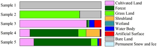
The evaluation of GDEM products is conducted over five selected areas in China, representing a broad range of geomorphological contexts, elevations and land cover types (Figure 1(f)). Each sample is defined by one 1° × 1° tile of analyzed GDEMs. Sample 1 is located at Taklamakan Desert in northwest China (Figure 1(a)). The area has a relatively flat topography with a mean terrain slope of 4.84°, and is covered by low dunes. This sample is nearly vegetation-free due to the extremely limited precipitation and high evaporation (Figure A1a), providing an ideal condition to compare the performances of GDEMs on the bare-earth surface. Sample 2 is situated at Qinghai-Tibet Plateau with an average altitude of more than 5000 m, characterized by steep mountains and broad valleys (Figure 1(b)). The area is mainly covered by grassland and bare land as well as sparse shrubs at relatively low elevations and permanent snow at high altitudes (Figure A1b). Sample 3 is located within the Jianghan Plain in central China, which is dominated by large-scale alluvium. It has a smooth and flat terrain with the lowest average elevation (30 m) among the five samples, with only a few gentle hills lying in the northwest region (Figure 1(c)). The agriculture is well developed and the cropland is the major land use type. The area is densely populated, with artificial surfaces and water bodies widely distributed (Figure A1c). Sample 4 and 5 are situated in the Hengduan Mountains in southwest China and southeast coastal areas of China, respectively. The vegetation in both samples is flourishing owing to the adequate rainfall and warm climate. Sample 4 has sheer and cliffy topography, with the greatest elevation range and average terrain slope (27.80°) among the five samples (Figure 1(d)). Because of the high latitude, the main land use types include forest, shrub, cropland and grass land (Figure A1d). Sample 5 is mountainous as well, though the topography is not as abrupt as sample 4, it has an average terrain slope of 22.77° (Figure 1(e)) and is mainly covered by dense forest (Figure A1e).

2.2. Datasets

2.2.1. Copernicus DEM

The Copernicus DEM is a 1-arcsec Digital Surface Model (DSM) based on the two radar satellite data acquired from December 2010 to January 2015 during the TanDEM-X mission. The primary goal of the mission is to create a worldwide, consistent and high-precision DSM using Synthetic Aperture Radar (SAR) interferometry (Fahrland et al. 2020). The mission provides DSM products at three resolutions (0.4″, 1″ and 3″). The 3″ Copernicus DEM was released in 2019, and 1″ DEM in late 2020, while the 0.4″ DEM was commercially available in 2016. The Copernicus DEM contains significant terrain correction and hydrological editing, such as spikes and holes removal, identification and filling of voids, edits of shore and coastlines, as well as correction of implausible terrain structures and random biases. The Copernicus DEM has been assessed against ICESat measurements, which indicates a vertical RMSE of 1.68 m (Leister-Taylor et al. 2020). The products are provided in Geographic Coordinates, with the horizontal reference datum of the World Geodetic System 1984 (WGS84), and the vertical reference datum of the Earth Gravitational Model 2008 (EGM2008).

2.2.2. NASADEM

The NASADEM is a void-free, near-global 1-arcsec elevation model that is generated by reprocessing of SRTM data. The main objective of the product is to eliminate voids and other limitations present in the SRTM by using datasets that are unavailable during the original processing. The improvements involve void reduction through improved phase unwrapping and better vertical control by referring to ICESat/GLAS elevations using a height error correction algorithm. Remnant voids are filled primarily by ASTER GDEM3 after merging the elevation data (Buckley et al. 2020). The NASADEM is supposed to be the successor of SRTM DEM, and expected to be more accurate and robust than the SRTM data (Crippen et al. 2016). The products are provided by 1° × 1° tiles with WGS84 geographic coordinates, and are relative to the Earth Gravitational Model of 1996 (EGM96).

2.2.3. AW3D DEM

The AW3D30 DEM is a free global optical stereoscopic DSM based on satellite images acquired by the Panchromatic Remote-sensing Instrument for Stereo Mapping (PRISM) onboard ALOS from January 2006 to April 2011 (Tadono et al. 2015). PRISM consists of three panchromatic radiometers that acquire along-track stereo images at nadir, forward and backwards, with a spatial resolution of 2.5 m. About 3 million images with cloud cover of less than 30% were used to produce the AW3D Standard DEM with a 5-m grid cell size (AW3D5) (Tadono et al. 2016). The AW3D30 is a resampled version of AW3D5 with a grid size of 1 arcsec, which was initially released in May 2016. The latest version 3.2 was made available in March 2021, which is adopted in this work. The data are provided in two formats: AVE (average) and MED (median), according to the different methods used for resampling from the 5-m mesh to the final released version. The AVE data are used for accuracy assessment, which are provided by 1° × 1° tiles with vertical reference to the EGM96 geoid and horizontal reference to the WGS84.

2.2.4. ICESAT-2

ICESat-2 is a follow-up mission to the successful ICESat mission. The spacecraft with ATLAS onboard operates in a 600 km orbit with a 91-day repeat cycle. The ATLAS is a photon counting lidar that transmits green (532 nm) laser with a detection sensitivity of individual photons. The instrument operates with three pairs of beams at a pulse repetition frequency of 10 kHz. Each pair is separated, approximately 3.3 km apart from each other with a pair spacing of 90 m, and consists of one high-energy beam and one low-energy beam (4:1 ratio) (Neuenschwander et al. 2020). Each of the beams generates overlapping footprints with a nominal diameter of 17 m, and an along-track sampling interval of 0.7 m (Neuenschwander and Magruder 2019). The configurations enable a much denser spatial sampling than its predecessor ICESat. The mission provides several geophysical products over various surface types. The land and vegetation height product (ATL08) is adopted in this work, which contains along-track heights for the ground and canopy surfaces. The slope corrected best-fit terrain height (h_te_bestfit) that represents the ground surface elevation is employed for the assessment. To ensure the quality of GCPs, the data acquired at night with the strong beam are used since they are less affected by the atmospheric scattering and solar background noise (Xiang et al. 2021). The product is processed in fixed 100 m segments, typically containing more than 100 signal photons. The ATL08 data (version 004) from October 2018 to July 2021 are downloaded from the National Snow and Ice Data Center (NSIDC) website, which are delivered in the WGS84 ellipsoidal and vertical datum.

3. Methods

3.1. Generation of reference dataset

The highly accurate GCP dataset is generated using ICESat-2/ATL08, which involves vertical datum conversion and outlier removal. As the ATL08 and GDEMs are referred to different vertical reference systems, a conversion has been applied to convert these datasets to a common orthometric system, the EGM96. For ATL08, the vertical datum is transformed from the WGS84 ellipsoid (h) to EGM96 heights (H) by using the geoid height (N), as follows: (1) $H=h-N$(1)

The ICESat-2 ATL08 data are then filtered to remove the outliers. ATL08 measurements are processed to exclude potential elevation anomalies which might result from cloud reflections using the cloud confidence flag. In addition, ATL08 points are compared with GDEM datasets to further exclude low-quality GCPs. For each point, the height difference $(\mathrm{\Delta }h)$ between the ATL08 and GDEM dataset is calculated. The ATL08 points are considered as outliers if the points with $\mathrm{\Delta }h$ outside the mean height difference $(\mathrm{\Delta }{h}_{mean})$ plus/minus three times standard deviation (STD) $(\mathrm{\Delta }{h}_{mean}\pm 3\ast STD)$. This approach is also known as the 3-sigma rule, which is widely used for outlier detection (Wessel et al. 2018; Hawker, Neal, and Bates 2019). As a result, more than 240,000 high-quality GCPs are generated for validating the GDEMs, with tens of thousands over each of the five study samples (Table 1, Figure 1).

Figure 1. Shaded relief maps of five studied tiles (a–e) based on Copernicus DEMs, showing landform features of different sites, and their locations in relation to China (f). The blue lines in each of the tiles are the high-quality ground control points used for the accuracy assessment, which are generated from ICESat-2 measurements.

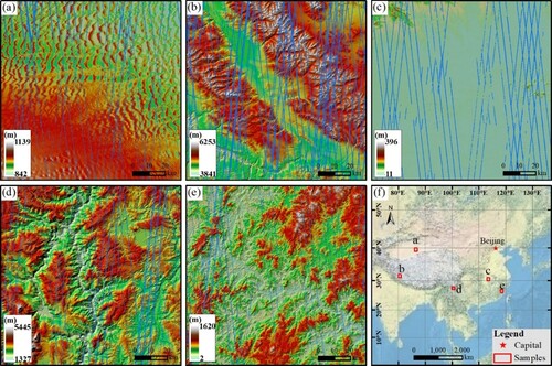
Table 1. The number of ICESat-2 GCPs generated for the GDEM assessment in the study samples.

GDEMs	Sample1	Sample2	Sample3	Sample4	Sample5	Total
Copernicus	35,748	82,109	34,510	57,129	30,888	240,384
NASA	35,961	81,634	34,707	57,297	30,901	240,500
AW3D30	35,853	82,002	34,632	57,296	30,895	240,678
Average	35,854	81,915	34,616	57,241	30,895

3.2. Accuracy assessment

The accuracy of GDEMs is assessed through both the visual inspection of terrain representation and the qualitative evaluation of vertical accuracy using generated GCPs. For some applications, the surface consistency and reliable rendering of terrain are important. These characteristics are referred to as a ‘shape and topologic quality’ (Polidori and El Hage 2020), also known as a ‘relative’ or ‘geomorphological’ accuracy (Szypuła 2019). However, standards for visually highlighting the problems in a DEM have not yet been formulized (Mesa-Mingorance and Ariza-López 2020). In this work, the colored shaded reliefs are generated for the GDEMs and then used to assess the geomorphological accuracy through visual analysis of certain landscape features, as suggested by previous studies (Guth and Geoffroy 2021). In addition, topographical profiles are also created to provide a comparison of elevation values.

Prior to the quantitative assessment, the vertical reference system of Copernicus DEM is transformed from EGM2008 to EGM96 to provide a consistent comparison. The conversion is carried out by calculating the geoid height differences between EMG96 and EGM2008 using the datum transformation tool (VDatum). As the value of DEM is referred to the elevation at the center of a pixel, which rarely corresponds to the location of GCP, the bilinear interpolation is applied to estimate the DEM elevation at the precise position of GCP. For each point, the error is calculated by subtracting the GCP elevation from that of the corresponding DEM. Positive values indicate areas where DEM is higher than the GCP, and vice versa. From these errors, three statistical metrics are reported, including the mean error (ME), standard deviation (STD), and RMSE, which are expressed as follows: (2) $\mathrm{ME}={\displaystyle \frac{{\sum }_{i=1}^n(Z_{DEM}-Z_{REF})}{n}}$(2) (3) $\mathrm{STD}=\sqrt{{\displaystyle \frac{{\sum }_{i=1}^n{[(Z_{DEM}-Z_{REF})-ME]}^2}{n-1}}}$(3) (4) $\mathrm{RMSE}=\sqrt{{\displaystyle \frac{{\sum }_{i=1}^n{(Z_{DEM}-Z_{REF})}^2}{n}}}$(4) where $Z_{DEM}$ refers to the elevation of GDEMs, $Z_{REF}$ refers to the reference elevation of ATL08 GCPs, and n is the number of points. In addition, the error histograms of the study samples are generated to illustrate the error distribution of GDEM.

To provide a better insight into the impact of terrain parameters on the vertical accuracy of GDEM, the error metrics are separately computed for individual slope ranges and land cover types. For this purpose, the slopes are derived from the DEM and then classified into seven ranges, including 0°–5°, 5°–10°, 10°–15°, 15°–20°, 20°–25°, 25°–30° and >30°. A 30-m global land cover dataset, GlobeLand30 V2020, is used to examine the effects of land cover (Chen et al. 2015). The dataset is derived from Landsat, HJ-1 and GF-1 images, which has a total of 10 land cover types and an overall classification accuracy of 85.72%. The GCPs are positioned within nine of these classes, including cultivated land, forest, grassland, shrub land, wetland, water body, artificial surfaces, bare land and permanent snow and ice. Moreover, the terrain-based land cover analysis is carried out to determine the predominant factor affecting the accuracy of DEM.

4. Results

4.1. Terrain representation

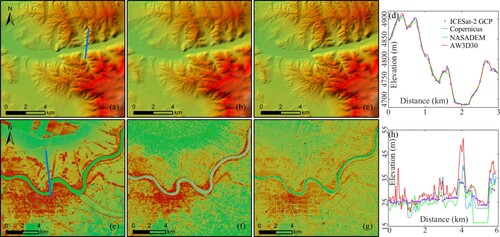
Figure 2 are the colorized shaded reliefs and topographic profiles of three GDEM subsets from a small rugged area in Sample 2 and a flat area in Sample 3. For the rugged terrain, all three GDEM subsets generally give a similar representation of relief (Figure 2(a–c)). A careful inspection shows that Copernicus DEM does the best job, with much sharper ridges and drainages, as well as much smoother valley floors, revealing the remarkable level of detail. AW3D30 comes in a close second, despite some noises present as artificial crests and sinks. Comparatively, NASADEM provides a blurry representation with low visual quality. The topographic profiles show that Copernicus and AW3D30 plot slightly above NASADEM, which is more consistent with ICESat-2 GCPs (Figure 2(d)). The flat terrain highlights the level of detail resolved by different GDEMs (Figure 2(e–g)). Located in a small city, it shows urban areas with a river flowing through. Some man-made features (e.g. elevated roads, canals, artificial levees, agricultural areas) can be identified in Copernicus and AW3D30 DEM, while they are barely seen in NASADEM. Similarly, AW3D30 DEM shows a noisy surface compared with Copernicus. The topographic profiles indicate that Copernicus DEM is most consistent with ICESat-2 GCPs, while AW3D30 overestimates and NASADEM underestimates the elevation in general (Figure 2(h)). The results reveal Copernicus and AW3D30 offer a high level of detail of terrain with an excellent representation while NASADEM provides a poor expression of terrain. This may be related to the original source of the products. The Copernicus DEM is derived from the 12 m resolution commercial TanDEM-X DEM, and the AW3D30 is a resampled version of the 5 m resolution AW3D5 DSM, while the NASADEM is produced from the 30 m SRTM DEM. Therefore, the effective spatial resolution of NASADEM is coarser than that of the other two GDEMs, which has also been addressed for SRTM by previous works (Guth 2006). The noises present in AW3D may be related to its source data, which have been reported to suffer from artificial noises (Purinton and Bookhagen 2017). The results reveal the differences of GDEMs in terrain representation and highlight its importance in quality assessment.

Figure 2. Visual assessment of terrain representation based on colorized shaded reliefs of three GDEM subsets from sample 2 (upper panel, elevation: 3840–6254 m) and sample 3 (bottom panel, elevation: 12–51 m), revealing different levels of detail resolved by GDEMs. (a, e) Copernicus DEM with indication of topographic profile location (blue line), (b, f) NASA and (c, g) AW3D30. Typical topographic profiles (north-south) and ICESat-2 GCPs are also plotted for the elevational comparison (d, h).

4.2. Vertical accuracy

Table 2 lists the error metrics of the three GDEMs and Figure 3 plots the corresponding error distributions. The results show that the three GDEMs have quite similar average vertical accuracy, with RMSE of 6.73, 6.59 and 6.63 m for Copernicus, NASA and AW3D30 DEM, respectively. The STD values are close to those of RMSE, which are 5.84, 6.34 and 5.59 m. The ME values are 3.35, 1.81 and 3.55 m, indicating that all the GDEMs overestimate the elevations compared to ICESat-2 GCPs. All three GDEMs show approximately narrow normal spread of errors with slightly positive biases, and the Copernicus has the narrowest peak with a bimodal distribution (Figure 3(f)). Although the DEMs have very similar overall accuracies, they vary considerably over the study areas and among GDEMs. All three GDEMs have better performances in Sample 1, 2 and 3 than those in Sample 4 and 5. Copernicus DEM performs the best in Sample 1, 2 and 3, and AW3D30 DEM is most accurate in Sample 4, while NASADEM provides the best accuracy in Sample 5. Error distributions indicate that all the DEMs have symmetric unimodal normal shapes in Sample 1, 2 and 3, while in Sample 4 and 5, they are right-skewed with a widespread of errors and the center of distribution shifted even further into positive values (Figure 3(a–e)). This is likely due to different combinations of slopes and land covers in the study areas (Figure A2-3), which will be investigated in detail in Section 4.3 and 4.4.

Figure 3. Histograms of vertical errors (GDEM - GCPs) for Copernicus, AW3D30 and NASA DEM by study samples. (a) Sample 1; (b) Sample 2; (c) Sample 3; (d) Sample 4; (e) Sample 5; (f) all five samples.

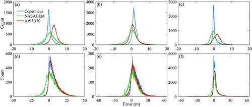
Table 2. Error metrics (in meters) of Copernicus, NASA and AW3D30 DEM for each of the five samples, including ME (Mean Error), STD (Standard Deviation), and RMSE (Root Mean Square Error).

Sites	Copernicus			NASA			AW3D30
	ME	STD	RMSE	ME	STD	RMSE	ME	STD	RMSE
Sample 1	−0.01	1.66	1.66	0.50	3.16	3.20	2.91	1.93	3.49
Sample 2	1.81	1.64	2.44	0.46	3.33	3.36	1.09	2.35	2.59
Sample 3	0.39	1.50	1.55	−0.39	1.72	1.77	1.78	2.20	2.83
Sample 4	6.78	7.52	10.12	4.48	9.06	10.10	6.79	7.17	9.87
Sample 5	8.32	8.52	11.91	4.43	9.16	10.17	6.82	8.59	10.97
Average	3.35	5.84	6.73	1.81	6.34	6.59	3.55	5.59	6.63

For Copernicus DEM, ME values range from −0.01 to 8.32 m with an average of 3.35 m. RMSE values vary from 1.55 to 11.91 m with an average of 6.73 m. The Copernicus DEM outperforms the other two DEMs in Sample 1, 2 and 3 with both low error values (Table 2) and narrow peaks in the error histograms (Figure 3(a–c)), where the study samples are sparsely vegetated with gentle slopes (Figure A2-3). However, Copernicus DEM shows the largest errors among the three GDEMs in Sample 4 and 5 with wide error distributions, suggesting its poor performance over rugged and densely vegetated areas. Although RMSE values of Copernicus DEM in Sample 1, 2 and 3 are the lowest, the average value is the highest among the three GDEMs.

For NASADEM, ME values range from −0.39 to 4.48 m with an average of 1.81 m. RMSE values vary from 3.20 to 10.17 m with an average of 6.34 m. The NASADEM has the lowest average ME and RMSE values among the three GDEMs. However, it has the largest STD values, revealing great uncertainties. Different from Copernicus, NASADEM has relatively small RMSE values in Sample 4 and 5, with the lowest RMSE of 10.17 m in Sample 5 among the three GDEMs, indicating that it performs better over vegetated and steep areas. Although the error distributions of NASADEM are the widest for four of the five samples (Figure 3(a–e)), the small error metrics in vegetated areas lead to the smallest average RMSE among the three GDEMs.

For AW3D30, ME values range from 1.09 to 6.82 m with an average of 3.55 m. The average ME of AW3D30 is the largest, suggesting that it is higher than the other two GDEMs. This is likely due to the weak penetration of optical sensors compared with that of the radar. The RMSE values vary from 2.59 to 10.97 m with an average of 6.63 m. Similar to NASADEM, AW3D30 has relatively small RMSE values in Sample 4 and 5, and performs best in Sample 4 with a RMSE of 9.87 m.

4.3. Terrain slope-based analysis

Figure 4 displays error measures of GDEMs for each slope class based on all the samples. The statistics are obtained using a sufficient number of GCPs, with over 20,000 for each of the classes. The results show an obvious relationship between the slope and DEM accuracy, with increasing slope leading to a worse accuracy compared with flatter areas. Accuracy variations are found among GDEMs. For NASADEM, it has the lowest ME values for all slope classes. While its STD values are the largest for all slope classes, it reveals the greatest uncertainties in NASADEM. For Copernicus DEM, it has lower ME values for areas with slope less than 10°, and larger values for slopes greater than 10° when compared with AW3D30. A similar trend is also observed in STD values. In terms of RMSE, Copernicus DEM is more accurate for gentle slopes (<10°) while NASA and AW3D30 DEM perform similarly better for slopes above 10°, and neither is consistently better than the other.

Figure 4. The vertical ME, STD, RMSE and the number of ICESat-2 GCPs for Copernicus, NASA and AW3D30 DEM by terrain slope classes based on all the five study samples (1: [0°–5°], 2: [5°–10°], 3: [10°–15°], 4: [15°–20°], 5: [25°–30°], 6: [25°–30°], 7: [>30°]).

Figure 5 presents error metrics of GDEMs by slope classes for each of the samples. It indicates that accuracy metrics vary greatly according to samples and GDEMs. For all the slope classes, all the GDEMs perform better in Sample 1, 2 and 3 than that in Sample 4 and 5, which are dominated by steep terrains (Figure A2). Although NASADEM has the lowest ME values for almost all the samples, it exhibits the largest STD values for four of the five samples. In terms of RMSE, Copernicus DEM performs the best for almost all the slope classes in Sample 1, 2 and 3 while only for flat areas (<5°) in Sample 4 and 5. AW3D30 DEM exhibits the worst accuracy in Sample 3 for all the slope classes. NASA and AW3D30 DEM show slightly better accuracies for slopes above 5° in Sample 4 and 5, and neither is consistently better than the other. For all the GDEMs, RMSE values increase slowly for gentle slopes but considerably for the steep. This is likely due to the additional effect of forests, which usually appears in rough mountain areas. The impact of land cover will be addressed in Section 4.4.

Figure 5. The vertical ME, STD, RMSE and the number of ICESat-2 GCPs for Copernicus, NASA and AW3D30 DEM by terrain slope classes over each of the five study samples (1: [0°–5°], 2: [5°–10°], 3: [10°–15°], 4: [15°–20°], 5: [25°–30°], 6: [25°–30°], 7: [>30°]).

4.4. Land cover-based analysis

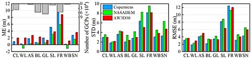
Figure 6 shows error metrics of GDEMs by land cover types based on all the samples. The statistics are derived from the GCPs that mainly fall in grassland, forest, bare land and cultivated land, with more than 40,000 for each of these types. The results exhibit some relationship between the accuracy and land covers. The ME values increase from negative for wetland and waterbody to more positive when vegetation is present. RMSEs also increase with vegetation, ranging from about 2 m for wetland, to about 11 m for forest. STDs exhibit a similar trend. Accuracies of GDEMs generally increase as the land cover changes from densely tall vegetation (forest) to moderate vegetation (shrub), and to sparsely low vegetation and open terrain (cultivated land, grassland, wetland, artificial surfaces, bare land). Accuracies are poor over dynamic land covers. For permanent snow and ice, errors of GDEMs are substantial for its rough terrain as well as variations in snow and ice cover. The accuracy of water body varies greatly, likely due to data voids and seasonal fluctuations. A similar trend is also observed for wetland, which exhibits seasonal hydrological cycles. The dynamic nature can be confirmed by ME values, which change from negative to positive for snow and ice, water body and wetland. Accuracy variations exist among GDEMs. NASADEM has the lowest ME and largest STD values for almost all the land cover types, which is the most accurate only for forest in terms of RMSE. Copernicus has the lowest STD values for almost all the land cover types, which is the most accurate for cultivated land, wetland, artificial surface, as well as waterbody and permanent snow and ice. AW3D30 provides the best accuracy for grassland and shrub land.

Figure 6. The vertical ME, STD, RMSE and the number of ICESat-2 GCPs for Copernicus, NASA and AW3D30 DEM by land cover types based on all five study samples (BL: bare land, CL: cultivated land, GL: grassland, WL: wetland, AS: artificial surfaces, SL: shrub land, FR: forest, WB: water body and SN: permanent snow and ice).

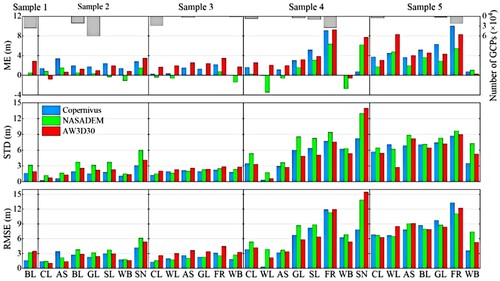
Figure 7 shows error statistics of GDEMs by land cover types for each of the samples. Accuracy metrics vary greatly according to both samples and GDEMs. For all the land cover types, all the GDEMs perform better in Sample 1, 2 and 3 than that in Sample 4 and 5. For permanent snow and ice, errors of GDEMs are the largest in the test sites (Sample 2 and 4). Errors of forest are substantial as the forest is mainly distributed in the steep mountains, adding more credit to its poor accuracy (Sample 4 and 5). NASADEM provides better accuracy than the other two GDEMs over the forest, despite the bad performance of the three GDEMs in this land cover. AW3D30 DEM exhibits the worst performance for all the land covers in Sample 3. It is noted that the sandy desert is considered as one of error sources that may affect the quality of interferometric SAR (InSAR) DEM, owing to weak backscattered returns from sandy regions (Rizzoli et al. 2017). However, it seems that this error is not significant as Copernicus and NASA DEM perform better than AW3D30 over sandy deserts in Sample 1. Overall, we can conclude that Copernicus DEM performs the best over bare land or sparsely low vegetation covers while NASADEM provides higher accuracy over the forest. It is observed that even for a specific land cover, performances of GDEMs vary among samples, which is likely due to variations in local terrain slopes. To identify the predominant factor, we further segment the results based on slope ranges, which will be addressed in Section 4.5.

Figure 7. The vertical ME, STD, RMSE and the number of ICESat-2 GCPs for Copernicus, NASA and AW3D30 DEM by land cover types over each of the five study samples (BL: bare land, CL: cultivated land, GL: grassland, WL: wetland, AS: artificial surfaces, SL: shrub land, FR: forest, WB: water body and SN: permanent snow and ice).

4.5. Terrain-based land cover analysis

Figure 8 shows the RMSE of major land cover types by slope classes for each of the GDEMs based on all the samples. For the major land cover types, accuracies of GDEMs generally decrease with the rise in slope classes. However, magnitudes are variable, revealing varying impacts of slope on accuracies of different land cover types. The accuracy of cultivated land is most impacted by slopes while bare land is least affected. RMSE values of cultivated land in Copernicus DEM increase by about 6 m when the slope class changes from 1 to 7, while a RMSE rise of only about 2 m for bare land (Figure 8(a)). For each of the slope classes, accuracies of GDEMs generally increase as land cover types change from forest to shrub land, cultivated land, grassland and bare land. Accuracies of land covers in each slope class are highly variable. In slope class 1 of Copernicus DEM, RMSEs range from about 2 m for cultivated land to a little bit over 8 m for forest, with a variation of approximately 6 m. While in class 7, RMSEs vary from 4 m for bare land to 14 m for forest, with a range of 10 m (Figure 8(a)). A similar trend can also be found in the other two GDEMs. Hence, the accuracy variation associated with land cover is much greater than that of the slope. This can also be confirmed by slope-based accuracy assessment results (Figure 5), where the accuracy of GDEM does not change significantly with the increase of slopes for bare land in Sample 1, suggesting the limited effect of terrain slopes. While it decreases greatly with the rise in slopes over densely vegetated areas (i.e. Sample 4), the importance of land covers is highlighted (Figure 5). It is worth noting that the influence of land cover varies among GDEMs. The land cover has a greater impact on the accuracy of Copernicus and AW3D30 than that of NASADEM (Figure 8). This is likely due to the stronger penetration capability of C-band waves, making NASADEM less impacted by various land covers. Overall, the results suggest that land cover has a greater influence on DEM accuracy than that of the slope in terms of our study area.

Figure 8. The vertical RMSE of major land cover types by slope classes for Copernicus (a), NASA (b) and AW3D30 DEM (c) based on all the study samples (FR: forest, SL: shrub land, CL: cultivated land, GL: grassland, BL: bare land; 1: [0°–5°], 2: [5°–10°], 3: [10°–15°], 4: [15°–20°], 5: [25°–30°], 6: [25°–30°], 7: [>30°]).

5. Discussions

5.1. ICESat-2 GCPs

It is generally acknowledged that the accuracy of the reference should be at least three times higher than that of the DEM under investigation (Athmania and Achour 2014). In this work, highly accurate ICESat-2 GCPs are generated from ICESat-2 ATL08 product. The product is the high-quality height estimates of topography (Neuenschwander and Pitts 2019). Validation results indicated that the accuracy of ATL08 terrain heights is within 0.70 m (Neuenschwander et al. 2020), compared to that of 2 m for ICESat (Huber et al. 2009). In the case of evaluated GDEMs, the vertical RMSEs are about 1.68 m (Copernicus), 5.5 m (NASA) and 4.4 m (AW3D30) according to the specifications of data producers (Leister-Taylor et al. 2020; Buckley et al. 2020; Tadono et al. 2016). In this work, additional procedures of quality filtering and outlier removal are applied to the generation of GCP dataset, which will provide even better accuracy and ensure a robust assessment. ICESat-2 ATL08 points have been increasingly used for DEM evaluation. Carabajal and Boy (2020) have shown that ICESat-2 ATL08 datasets are of sufficient accuracy to create global GCPs for the quality evaluation of DEM. Guth and Geoffroy (2021) have demonstrated that accuracy assessment results using ICESat-2 are comparable to those using LiDAR DEMs, which typically has a vertical accuracy of less than 20 cm. In addition, a large quantity of generated GCPs (more than 240,000) overcomes the frequent criticism that the accuracy is assessed by a limited number of surveyed GCPs (Höhle and Höhle 2009), and therefore makes the results less affected by pixel sparsity. Regarding this issue, Vassilaki and Stamos (2020) also suggest using LiDAR data rather than sparse points such as GPS observations to guarantee reliable conclusions. As for ICESat-2, the orbital configuration of monthly sub-cycles enables lateral data collection shift, which increases the coverage area and provides denser elevation measurements over time. Furthermore, the generated GCPs are evenly distributed across the study areas (Figure 1), allowing an unbiased assessment over various terrains and land covers. To this end, advantages of ICESat-2 as reference data are evident, providing a sufficient high accuracy and large quantity for a robust validation, as well as its global availability free of charge. In short, ICESat-2 altimetry has proven to be a valuable tool for DEM assessment, which highlights the discrepancies among the three newly released 1-arcsec GDEMs.

5.2. Overall accuracy

Our results suggest that the three GDEMs have nearly identical overall accuracy metrics with RMSE of about 6.6 m when considering all five samples, and the accuracies of GDEMs are highly variable, with RMSE ranging from 1.55 to 11.91 m (Table 2). Our findings are generally consistent with previous works, despite the fact that they are very limited for the three newly available GDEMs. Grohmann (2018) compared 30 m TanDEM-X, SRTM, ASTER GDEM and AW3D30 DEMs with 12 m TanDEM-X DEM over seven Brazilian sites. He found that TanDEM-X 30 m showed smaller deviations from the reference. SRTM 30 m showed the RMSE between 3.11 and 8.24 m and AW3D30 had RMSE ranging from 2.75 to 9.43 m. Uuemaa et al. (2020) conducted the vertical accuracy assessment of six GDEMs (ASTER, AW3D30, MERIT, TanDEM-X, SRTM and NASADEM) using LiDAR DEM as reference. Results showed that AW3D30 offered the most stable and accurate elevation data, with RMSE of 7.92, 7.18 and 11.42 m in study areas from Estonia, China, and New Zealand, respectively, while those of NASADEM were 6.39, 8.53 and 12.08 m, showing slightly better accuracy than SRTM DEM. González-Moradas and Viveen (2020) assessed the vertical accuracy of three 30 m DEMs (ASTER GDEM2, SRTM3, AW3D30) and one 12 m DEM (TanDEM-X) for the Peruvian Andes against 139 GCPs. The overall accuracy showed that the RMSE values were 6.91 (ASTER), 5.11 (SRTM3) and 6.25 m (AW3D30). Carrera-Hernández (2021) evaluated the vertical accuracy of eight DEMs available for Mexico (AW3D30, ASTER, SRTM, NASADEM and Mexico’s Continuous Elevation Model (CEM)) using LiDAR DEM as reference. Results indicated that the AW3D30 provided the best accuracy (MAE = 2.5 m), followed by NASADEM (3.1 m), SRTM (3.8 m), CEM (4.6 m) and ASTER GDEM3 (6.0 m). Most of the aforementioned studies suggest that both NASA and AW3D30 DEM have similar accuracy, with error metrics varying from a few (i.e. Carrera-Hernández 2021) to about 6 m (i.e. Uuemaa et al. 2020; González-Moradas and Viveen 2020), compared to that of ∼6.6 m in this work. The slight discrepancies between previous works and our study may be related to different study areas and different land covers (i.e. water body is excluded in some works) as well as different reference data.

Our study reveals that Copernicus DEM is more accurate over flat terrains featured by bare land or sparse vegetation, and offers the best representation of terrain with the highest level of detail (Figure 4, Figure 2). The accuracy assessment work of Copernicus DEM is very limited. Guth and Geoffroy (2021) compared five 1-arcsec GDEMs (Copernicus, AW3D30, ASTER, NASA and SRTM) against LiDAR point clouds, and found that Copernicus DEM outperformed the other four GDEMs because it had very few points outside the point cloud. However, the accuracy metrics were not provided in their work. Moreover, they found that Copernicus did the best job for terrain representation. Purinton and Bookhagen (2021) assessed inter-pixel variability of five 1- arcsec GDEMs (SRTM, ASTER, ALOS, TanDEM-X and Copernicus) in the arid steep Central Andes, and suggested that Copernicus DEM provided the highest quality of landscape representation. Our findings are in line with previous findings in terrain representation, and provide quantitative assessment results for Copernicus DEM with regards to various terrain slopes and land covers.

5.3. Terrain parameters

The terrain slope related accuracy variations of spaceborne GDEMs are likely due to geometric distortions of satellite images as well as errors caused by horizontal offsets. The distortions often occur over steep and irregular surfaces that are closely related to terrain slopes. The steeper the slope is, the more distorted the images will be. The distortions make the matching of stereo SAR and optical images more difficult and less accurate, and hence impact the accuracy of resultant GDEM (González-Moradas and Viveen 2020). In addition, the vertical accuracy may also be affected by horizontal errors. Small horizontal offsets are often observed in GCPs and among GDEMs (Neuenschwander et al. 2020; Li, Deng, and Wang 2017). The horizontal shift associated vertical error $({\epsilon }_{ZH})$ can be calculated by a function of local slope $(\alpha )$ and horizontal error $({\epsilon }_H)$, expressed as ${\epsilon }_{ZH}={\epsilon }_H\tan \alpha$ (Hodgson et al. 2005). The associated errors are insignificant when terrain slopes are gentle, but will increase rapidly if the slope is greater than 45°, and even reach infinity as slope approaches 90°. Overall, the accuracy of spaceborne DEM decreases with the increase of slope as a result of image matching errors and horizontal shift associated errors. Many of the previous works reported a similar relationship between terrain slope and DEM accuracy (Li and Zhao 2018; Grohmann 2018; Uuemaa et al. 2020; González-Moradas and Viveen 2020). Specifically, Wessel et al. (2018) also showed a considerable increase of RMSEs over slopes above 10° for TanDEM-X DEM, which has the same data source as Copernicus DEM.

The impact of land cover on the accuracy of GDEMs may be related to different penetration abilities of satellite sensors. For bare land and sparsely low vegetation, both optical and radar sensors as well as ICESat-2 photons can penetrate and track the ground surface (Neuenschwander et al. 2020). Hence, all three GDEMs exhibit high accuracies in these land covers (Figure 6). For tall and dense vegetation (i.e. forest), long C-band waves (5.6 cm in wavelength) are found to penetrate significantly into the canopy while short X-band (3.1 cm in wavelength) and optical signals show limited penetration capabilities (Walker, Kellndorfer, and Pierce 2007; Magruder, Neuenschwander, and Klotz 2021). In contrast, ICESat-2 photons can penetrate the canopy and track the ground surface (Neuenschwander and Pitts 2019). As a result, positions measured by X-band and optical waves are located somewhere around the top of canopy, while those detected by C-band are inside the vegetation layer, which are closer to the ground tracked by ICESat-2 photons. Therefore, NASADEM has the smallest ME values for most of the land covers, and performs the best over forest among the three GDEMs (Figure 6). Overall, accuracy variations caused by land covers can be largely explained by different penetration capacities of corresponding sensors. To this end, NASADEM is more likely to be regarded as a DTM (Digital Terrain Model) in the sense that the C-band signal can measure the surface close to the ground even in the forest canopy. AW3D30 and Copernicus DEM fail to depict the ‘bare’ ground in dense vegetated areas, and therefore can be referred to as a DSM rather than a DTM. Our results are coherent with previous findings. Carabajal and Boy (2020) found that SRTM DEM measured 0.76 m above the ICESat-2 defined surface for hard ground, and 8.41 m for broadleaf forest, with variability rising with the increased percentage of tree cover. Guth and Geoffroy (2021) revealed that accuracies of DEMs increased as the land cover changed from closed forest to open forest and short vegetation, due to variable penetration depths of sensors through different land covers.

The terrain-based land cover analysis suggests that land cover type is the predominant factor that affects the accuracy of DEM. However, previous studies found that terrain relief exerts a greater influence (Li and Zhao 2018; Liu et al. 2019). We argue that the discrepancies may be ascribed to different terrain characteristics of study sites. For areas without any land covers (i.e. desert), the terrain slope would exert a greater impact on the DEM accuracy. As for areas with very gentle slopes (i.e. plain), land cover type might play a bigger role. While for complex areas with both rugged reliefs and diverse land cover types, terrain-based land cover analysis allows a detailed investigation and determines the major contribution factor.

5.4. Limitation and recommendation

This work does not consider temporal changes among the reference and GDEM datasets, which span from the present ICESat-2 GCPs to the NASADEM of two decades ago. Some have very short intervals of data collection, such as NASADEM, while others take multiple years, such as Copernicus and AW3D30 DEM (Guth and Geoffroy 2021). Hence, considerable temporal inconsistencies exist among these datasets, and potential elevation changes in some areas may occur, especially over those with highly dynamic natures (i.e. snow and ice, water body and wetland) as well as urban areas (i.e. artificial surfaces), which would affect the assessment results. In this work, we only focus on the vertical accuracy and do not consider the horizontal displacement, which may impact the vertical accuracy. According to Li and Zhao (2018), the vertical accuracies are improved following the alignment of GDEMs, with the decrease of RMSE by 0.58 and 0.37 m for SRTM and ASTER GDEM, respectively. Thus, it is likely that the sub-pixel horizontal displacement has little impact on the vertical accuracy. It is noted that although the five study tiles in China might be geographically limited, they are diverse in terms of reliefs, vegetation and land covers, ranging from the gently sloping alluvial plain (Sample 3) to highly rugged mountains (Sample 4), and from the bare land in desert (Sample 1) to densely vegetated regions (Sample 5). The assessment results are therefore presumed to be a good indication of the performances of GDEMs over other regions of the world, providing a good understanding of the potential and limitations of the three products.

Although the three GDEMs have similar overall vertical accuracy, they vary highly from one another depending on local terrain parameters. Therefore, users should take into consideration terrain characteristics of the area under investigation when choosing a proper GDEM. If the area is mainly gentle terrains covered by bare ground, shrub land, urban areas and sparse vegetation, Copernicus DEM would be the most accurate. For areas with rugged reliefs dominated by dense vegetation, NASA and AW3D30 DEM provide similar and better accuracy. As for terrain representation, Copernicus DEM should be the first choice, followed by AW3D30 DEM. Our findings of relationships between GDEM accuracies and terrain parameters may have important implications for the improvement of GDEMs, which could be used to develop terrain-specific or land cover-orientated algorithms to correct the GDEMs.

6. Conclusion

This work presents a timely and comprehensive accuracy assessment of three newly released 1-arcsec global DEMs in the five selected study samples of China with distinct geomorphological contexts, vegetation and land cover, using more than 240,000 high-quality GCPs generated from the ICESat-2 ALT08 product. The results show that the three GDEMs provide the similar overall vertical accuracies, with RMSE of 6.73 (Copernicus), 6.59 (NASA) and 6.63 m (AW3D30). However, performances vary greatly from one to another in the five study areas, likely due to different combinations of terrain and land cover in each of the validation sites. Further investigation into the vertical accuracy and terrain parameters reveals a good correlation between the accuracy and terrain slope, with the rise in slope leading to a decrease in accuracy. Copernicus DEM outperforms NASA and AW3D30 DEM in the low-relief areas, while the latter two show better performances over steep areas. Results also indicate relevance between accuracy and land covers. Accuracy increases as the land cover type changes from densely tall vegetation to sparsely low vegetation and open terrain. NASADEM provides the best accuracy in dense forest, while Copernicus DEM performs the best in land covers of bare land and sparsely vegetation. This may be related to the fact that the C-band SAR of NASADEM can penetrate much deeper into vegetation canopies than those of X-band of Copernicus DEM and optical band of AW3D30. The terrain-based land cover analysis allows the determination of major factor affecting DEM accuracy, which reveals that the land cover type exerts greater influence than that of the terrain slope for the study area, and also suggests that the impact of land cover on accuracy varies among the three GDEMs. Visual inspection of terrain representation indicates that Copernicus DEM exhibits the greatest detail of terrain, followed by AW3D30, while NASADEM offers the worst topography presentation quality. The results obtained suggest that users should take into consideration terrain characteristics of the area under investigation when choosing a proper DEM. This work has also demonstrated that ICESat-2 altimetry is an important assessment tool for GDEMs, which highlights the differences among the GDEMs.

Acknowledgements

This work was supported by the National Natural Science Foundation of China (41201429, 42171375). The authors gratefully thank the data distribution agencies for providing the test data. We thank Ms Y. H. Liu for her assistance with English language editing. The authors would also like to thank the editors and the anonymous reviewers for their valuable suggestions, which helped us make major improvements to this manuscript.

Disclosure statement

No potential conflict of interest was reported by the author(s).

Additional information

Funding

This work was supported by the National Natural Science Foundation of China [grant number 41201429, 42171375].

Appendices

Figure A1. Land cover type maps for each of the five study tiles.

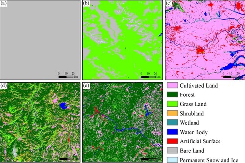
Figure A2. Combination of terrain slope classes for each of the study areas.

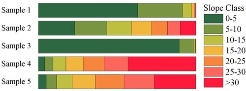
Figure A3. Combination of land cover types for each of the study areas.

References

- Athmania, D., and H. Achour. 2014. “External Validation of the ASTER GDEM2, GMTED2010 and CGIAR–CSI– SRTM v4.1 Free Access Digital Elevation Models (DEMs) in Tunisia and Algeria.” Remote Sensing 6 (5): 4600–4620. doi:10.3390/rs6054600.
- Berry, P. A. M., J. D. Garlick, and R. G. Smith. 2007. “Near-Global Validation of the SRTM DEM Using Satellite Radar Altimetry.” Remote Sensing of Environment 106 (1): 17–27. doi:10.1016/j.rse.2006.07.011.
- Berthier, E., Y. Arnaud, R. Kumar, S. Ahmad, P. Wagnon, and P. Chevallier. 2007. “Remote Sensing Estimates of Glacier Mass Balances in the Himachal Pradesh (Western Himalaya, India).” Remote Sensing of Environment 108 (3): 327–338. doi:10.1016/j.rse.2006.11.017.
- Bhang, K. J., F. W. Schwartz, and A. Braun. 2007. “Verification of the Vertical Error in C-Band SRTM DEM Using ICESat and Landsat-7, Otter Tail County, MN.” IEEE Transactions on Geoscience and Remote Sensing 45 (1): 36–44. doi:10.1109/tgrs.2006.885401.
- Buckley, S. M., P. S. Agram, J. E. Belz, R. E. Crippen, E. M. Gurrola, S. Hensley, M. Kobrick, et al. 2020. “NASADEM: User Guide.” NASA JPL: Pasadena, January. https://lpdaac.usgs.gov/documents/592/NASADEM_User_Guide_V1.pdf
- Carabajal, C. C., and J. P. Boy. 2020. “Icesat-2 Altimetry as Geodetic Control.” The International Archives of the Photogrammetry, Remote Sensing and Spatial Information Sciences XLIII-B3-2020: 1299–1306. doi:10.5194/isprs-archives-XLIII-B3-2020-1299-2020.
- Carrera-Hernández, J. J. 2021. “Not All DEMs Are Equal: An Evaluation of Six Globally Available 30 m Resolution DEMs with Geodetic Benchmarks and LiDAR in Mexico.” Remote Sensing of Environment 261, 112474. doi:10.1016/j.rse.2021.112474.
- Chen, J., J. Chen, A. Liao, X. Cao, L. Chen, X. Chen, C. He, et al. 2015. “Global Land Cover Mapping at 30 m Resolution: A POK-Based Operational Approach.” ISPRS Journal of Photogrammetry and Remote Sensing 103: 7–27. doi:10.1016/j.isprsjprs.2014.09.002.
- Crippen, R., S. Buckley, P. Agram, E. Belz, E. Gurrola, S. Hensley, M. Kobrick, et al. 2016. “NASADEM Global Elevation Model: Methods and Progress.” ISPRS - International Archives of the Photogrammetry, Remote Sensing and Spatial Information Sciences XLI-B4: 125–128. doi:10.5194/isprsarchives-XLI-B4-125-2016.
- Fahrland, E., P. Jacob, H. Schrader, and H. Kahabka. 2020. “Copernicus DEM Product Handbook.” June 25. https://spacedata.copernicus.eu/documents/20126/0/GEO1988-CopernicusDEM-SPE-002_ProductHandbook_I1.00.pdf.
- Farr, T. G., P. A. Rosen, E. Caro, R. Crippen, R. Duren, S. Hensley, M. Kobrick, et al. 2007. “The Shuttle Radar Topography Mission.” Reviews of Geophysics 45 (2): RG2004. doi:10.1029/2005rg000183.
- González-Moradas, M. D. R., and W. Viveen. 2020. “Evaluation of ASTER GDEM2, SRTMv3.0, ALOS AW3D30 and TanDEM-X DEMs for the Peruvian Andes Against Highly Accurate GNSS Ground Control Points and Geomorphological-Hydrological Metrics.” Remote Sensing of Environment 237: 111509. doi:10.1016/j.rse.2019.111509.
- Gorokhovich, Y., and A. Voustianiouk. 2006. “Accuracy Assessment of the Processed SRTM-Based Elevation Data by CGIAR Using Field Data from USA and Thailand and Its Relation to the Terrain Characteristics.” Remote Sensing of Environment 104 (4): 409–415. doi:10.1016/j.rse.2006.05.012.
- Grohmann, C. H. 2018. “Evaluation of TanDEM-X DEMs on Selected Brazilian Sites: Comparison with SRTM, ASTER GDEM and ALOS AW3D30.” Remote Sensing of Environment 212: 121–133. doi:10.1016/j.rse.2018.04.043.
- Guth, P. L. 2006. “Geomorphometry from SRTM.” Photogrammetric Engineering and Remote Sensing 72 (3): 269–277. doi:10.14358/pers.72.3.269.
- Guth, P. L., and T. M. Geoffroy. 2021. “LiDAR Point Cloud and ICESat-2 Evaluation of 1 Second Global Digital Elevation Models: Copernicus Wins.” Transactions in GIS 25 (5): 2245–2261. doi:10.1111/tgis.12825.
- Hawker, L., P. Bates, J. Neal, and J. Rougier. 2018. “Perspectives on Digital Elevation Model (DEM) Simulation for Flood Modeling in the Absence of a High-Accuracy Open Access Global DEM.” Frontiers in Earth Science 6: 233. doi:10.3389/feart.2018.00233.
- Hawker, L., J. Neal, and P. Bates. 2019. “Accuracy Assessment of the TanDEM-X90 Digital Elevation Model for Selected Floodplain Sites.” Remote Sensing of Environment 232: 111319. doi:10.1016/j.rse.2019.111319.
- Heras, M. M., P. M. Saco, and G. R. Willgoose. 2012. “A Comparison of SRTM V4 and ASTER GDEM for Hydrological Applications in Low Relief Terrain.” Photogrammetric Engineering and Remote Sensing 78 (7): 757–766. doi:10.14358/PERS.78.7.757.
- Hodgson, M. E., J. Jensen, G. Raber, J. Tullis, B. A. Davis, G. Thompson, and K. Schuckman. 2005. “An Evaluation of Lidar-derived Elevation and Terrain Slope in Leaf-off Conditions.” Photogrammetric Engineering and Remote Sensing 71 (7): 817–823. doi:10.14358/pers.71.7.817.
- Höhle, J., and M. Höhle. 2009. “Accuracy Assessment of Digital Elevation Models by Means of Robust Statistical Methods.” ISPRS Journal of Photogrammetry and Remote Sensing 64 (4): 398–406. doi:10.1016/j.isprsjprs.2009.02.003.
- Huber, M., B. Wessel, D. Kosmann, A. Felbier, V. Schwieger, M. Habermeyer, A. Wendleder, and A. Roth. 2009. “Ensuring Globally the TanDEM-X Height Accuracy: Analysis of the Reference Data Sets ICESat, SRTM and KGPS-Tracks.” Paper presented at the 2009 IEEE International Geoscience and Remote Sensing symposium, 12–17 July. doi:10.1109/igarss.2009.5418204.
- Ivanov, M. A., and O. P. Yermolaev. 2017. “Geomorphometric Analysis of River Basins of the Volga Federal District Using SRTM and ASTER GDEM Data.” Journal of Engineering and Applied Sciences 14 (2): 98–109. doi:10.21046/2070-7401-2017-14-2-98-109.
- Leister-Taylor, V., P. Jacob, H. Schrader, and H. Kahabka. 2020. “Copernicus DEM Validation Report.” November 9. https://spacedata.copernicus.eu/documents/20126/0/GEO1988-CopernicusDEM-RP-001_ValidationReport_I3.0.pdf.
- Li, H., X. Chen, J. Kyoung, X. Cai, and S. Myung. 2010. “Assessment of Soil Erosion and Sediment Yield in Liao Watershed, Jiangxi Province, China, Using USLE, GIS, and RS.” Journal of Earth Science 21 (6): 941–953. doi:10.1007/s12583-010-0147-4.
- Li, H., Q. Deng, and L. Wang. 2017. “Automatic Co-Registration of Digital Elevation Models Based on Centroids of Subwatersheds.” IEEE Transactions on Geoscience and Remote Sensing 55 (11): 6639–6650. doi:10.1109/TGRS.2017.2731048.
- Li, H., X. Huang, Q. Deng, T. M. Kusky, and X. Cai. 2012. “Mapping of Planation Surfaces in the Southwest Region of Hubei Province, China – Using the DEM-Derived Painted Relief Model.” Journal of Earth Science 23 (5): 719–730. doi:10.1007/s12583-012-0290-1.
- Li, H., and J. Zhao. 2018. “Evaluation of the Newly Released Worldwide AW3D30 DEM over Typical Landforms of China Using Two Global DEMs and ICESat/GLAS Data.” IEEE Journal of Selected Topics in Applied Earth Observations and Remote Sensing 11 (11): 4430–4440. doi:10.1109/JSTARS.2018.2874361.
- Liu, X. 2008. “Airborne LiDAR for DEM Generation: Some Critical Issues.” Progress in Physical Geography: Earth and Environment 32 (1): 31–49. doi:10.1177/0309133308089496.
- Liu, K., C. Song, L. Ke, L. Jiang, Y. Pan, and R. Ma. 2019. “Global Open-Access DEM Performances in Earth’s Most Rugged Region High Mountain Asia: A Multi-Level Assessment.” Geomorphology 338: 16–26. doi:10.1016/j.geomorph.2019.04.012.
- Magruder, L., A. Neuenschwander, and B. Klotz. 2021. “Digital Terrain Model Elevation Corrections Using Space-Based Imagery and ICESat-2 Laser Altimetry.” Remote Sensing of Environment 264: 112621. doi:10.1016/j.rse.2021.112621.
- Mesa-Mingorance, J. L., and F. J. Ariza-López. 2020. “Accuracy Assessment of Digital Elevation Models (DEMs): A Critical Review of Practices of the Past Three Decades.” Remote Sensing 12 (16): 2630. doi:10.3390/rs12162630.
- Mukul, M., V. Srivastava, S. Jade, and M. Mukul. 2017. “Uncertainties in the Shuttle Radar Topography Mission (SRTM) Heights: Insights from the Indian Himalaya and Peninsula.” Scientific Reports 7 (1): 41672. doi:10.1038/srep41672.
- Neuenschwander, A., E. Guenther, J. C. White, L. Duncanson, and P. Montesano. 2020. “Validation of ICESat-2 Terrain and Canopy Heights in Boreal Forests.” Remote Sensing of Environment 251: 112110. doi:10.1016/j.rse.2020.112110.
- Neuenschwander, A. L., and L. A. Magruder. 2019. “Canopy and Terrain Height Retrievals with ICESat-2: A First Look.” Remote Sensing 11 (14): 1721. doi:10.3390/rs11141721.
- Neuenschwander, A., and K. Pitts. 2019. “The ATL08 Land and Vegetation Product for the ICESat-2 Mission.” Remote Sensing of Environment 221: 247–259. doi:10.1016/j.rse.2018.11.005.
- Nikolakopoulos, K. G. 2020. “Accuracy Assessment of ALOS AW3D30 DSM and Comparison to ALOS PRISM DSM Created with Classical Photogrammetric Techniques.” European Journal of Remote Sensing 53 (sup2): 39–52. doi:10.1080/22797254.2020.1774424.
- Polidori, L., and M. El Hage. 2020. “Digital Elevation Model Quality Assessment Methods: A Critical Review.” Remote Sensing 12 (21): 2522. doi:10.3390/rs12213522.
- Purinton, B., and B. Bookhagen. 2017. “Validation of Digital Elevation Models (DEMs) and Comparison of Geomorphic Metrics on the Southern Central Andean Plateau.” Earth Surface Dynamics 5 (2): 211–237. doi:10.5194/esurf-5-211-2017.
- Purinton, B., and B. Bookhagen. 2021. “Beyond Vertical Point Accuracy: Assessing Inter-Pixel Consistency in 30 m Global DEMs for the Arid Central Andes.” Frontiers in Earth Science 9: 758606. doi:10.3389/feart.2021.758606.
- Rizzoli, P., M. Martone, C. Gonzalez, C. Wecklich, D. B. Tridon, B. Bräutigam, M. Bachmann, et al. 2017. “Generation and Performance Assessment of the Global TanDEM-X Digital Elevation Model.” ISPRS Journal of Photogrammetry and Remote Sensing 132: 119–139. doi:10.1016/j.isprsjprs.2017.08.008.
- Saksena, S., and V. Merwade. 2015. “Incorporating the Effect of DEM Resolution and Accuracy for Improved Flood Inundation Mapping.” Journal of Hydrology 530: 180–194. doi:10.1016/j.jhydrol.2015.09.069.
- Satge, F., M. Denezine, R. Pillco, F. Timouk, S. Pinel, J. Molina, J. Garnier, F. Seyler, and M. P. Bonnet. 2016. “Absolute and Relative Height-Pixel Accuracy of SRTM-GL1 over the South American Andean Plateau.” ISPRS Journal of Photogrammetry and Remote Sensing 121: 157–166. doi:10.1016/j.isprsjprs.2016.09.003.
- Szypuła, B. 2019. “Quality Assessment of DEM Derived from Topographic Maps for Geomorphometric Purposes.” Open Geosciences 11 (1): 843–865. doi:10.1515/geo-2019-0066.
- Tachikawa, T., M. Hato, M. Kaku, and A. Iwasaki. 2011. “Characteristics of ASTER GDEM Version 2.” Paper presented at the 2011 IEEE International Geoscience and Remote Sensing symposium, 24–29 July 2011. doi:10.1109/igarss.2011.6050017.
- Tadono, T., H. Nagai, H. Ishida, F. Oda, S. Naito, K. Minakawa, and H. Iwamoto. 2016. “Generation of the 30 M-Mesh Global Digital Surface Model by ALOS PRISM.” ISPRS - International Archives of the Photogrammetry, Remote Sensing and Spatial Information Sciences XLI-B4: 157–162. doi:10.5194/isprsarchives-XLI-B4-157-2016.
- Tadono, T., J. Takaku, K. Tsutsui, F. Oda, and H. Nagai. 2015. “Status of “ALOS World 3D (AW3D)” Global DSM Generation.” Paper presented at the 2015 IEEE International Geoscience and Remote Sensing Symposium (IGARSS), 26–31 July 2015. doi:10.1109/igarss.2015.7326657.
- Tarolli, P. 2014. “High-Resolution Topography for Understanding Earth Surface Processes: Opportunities and Challenges.” Geomorphology 216: 295–312. doi:10.1016/j.geomorph.2014.03.008.
- Unwin, D. J. 1995. “Geographical Information Systems and the Problem of ‘Error and Uncertainty’.” Progress in Human Geography 19 (4): 549–558. doi:10.1177/030913259501900408.
- Uuemaa, E., S. Ahi, B. Montibeller, M. Muru, and A. Kmoch. 2020. “Vertical Accuracy of Freely Available Global Digital Elevation Models (ASTER, AW3D30, MERIT, TanDEM-X, SRTM, and NASADEM).” Remote Sensing 12 (21): 3482. doi:10.3390/rs12213482.
- Vassilaki, D. I., and A. A. Stamos. 2020. “TanDEM-X DEM: Comparative Performance Review Employing LiDAR Data and DSMs.” ISPRS Journal of Photogrammetry and Remote Sensing 160: 33–50. doi:10.1016/j.isprsjprs.2019.11.015.
- Vieceli, N., T. A. Bortolin, L. A. Mendes, G. Bacarim, G. Cemin, and V. E. Schneider. 2015. “Morphometric Evaluation of Watersheds in Caxias do Sul City, Brazil, Using SRTM (DEM) Data and GIS.” Environmental Earth Sciences 73 (9): 5677–5685. doi:10.1007/s12665-014-3823-3.
- Walker, W. S., J. M. Kellndorfer, and L. E. Pierce. 2007. “Quality Assessment of SRTM C- and X-Band Interferometric Data: Implications for the Retrieval of Vegetation Canopy Height.” Remote Sensing of Environment 106 (4): 428–448. doi:10.1016/j.rse.2006.09.007.
- Wessel, B., M. Huber, C. Wohlfart, U. Marschalk, D. Kosmann, and A. Roth. 2018. “Accuracy Assessment of the Global TanDEM-X Digital Elevation Model with GPS Data.” ISPRS Journal of Photogrammetry and Remote Sensing 139: 171–182. doi:10.1016/j.isprsjprs.2018.02.017.
- Xiang, J., H. Li, J. Zhao, X. Cai, and P. Li. 2021. “Inland Water Level Measurement from Spaceborne Laser Altimetry: Validation and Comparison of Three Missions Over the Great Lakes and Lower Mississippi River.” Journal of Hydrology 597: 126312. doi:10.1016/j.jhydrol.2021.126312.
- Yue, L., W. Yu, H. Shen, L. Zhang, and Y. He. 2015. “Accuracy Assessment of SRTM V4.1 and ASTER GDEM V2 in High-Altitude Mountainous Areas: A Case Study in Yulong Snow Mountain, China.” Paper presented at the 2015 IEEE International Geoscience and Remote Sensing Symposium (IGARSS), 26–31 July 2015. doi:10.1109/igarss.2015.7326958.
- Zwally, H. J., B. Schutz, W. Abdalati, J. Abshire, C. Bentley, A. Brenner, J. Bufton, et al. 2002. “ICESat’s Laser Measurements of Polar Ice, Atmosphere, Ocean, and Land.” Journal of Geodynamics 34 (3): 405–445. doi:10.1016/S0264-3707(02)00042-X.