Variation of XCO₂ anomaly patterns in the Middle East from OCO-2 satellite data

ABSTRACT

The anthropogenic CO₂ emission is contributed to the rapid increase in CO₂ concentration. In the current study the anthropogenic CO₂ emission in the Middle East (ME) is investigated using 6 years column-averaged CO₂ dry air mole fraction (XCO₂) observation from Orbiting Carbon Observatory-2 (OCO-2) satellite. In this way, the XCO₂ anomaly ($\mathrm{\Delta }$XCO₂) as the detrended and deseasonalized term of OCO-2XCO₂ product, was computed and compared to provide the direct space-based anthropogenic CO₂ emission monitoring. As a result, the high positive and negative $\mathrm{\Delta }$XCO₂ values have corresponded to the major sources such as oil and gas industries, and growing seasons over ME, respectively. Consequently, the Open-source Data Inventory for Anthropogenic CO₂ (ODIAC) emission and the gross primary productivity (GPP) were utilized in exploring the $\mathrm{\Delta }$XCO₂ relation with human and natural driving factors. The results showed the capability of $\mathrm{\Delta }$XCO₂ maps in detecting CO₂ emission fluctuations in defined periods were detectible in daily to annual periods. The simplicity and accuracy of the method in detecting the man-made and natural driving factors including the main industrial areas, megacities, or local changes due to COVID-19 pandemic or geopolitical situations as well as the vegetation absorption and biomass burning is the key point that provides the environmental managers and policymakers with valuable and accessible information to control and ultimately reduce the CO₂ emission over critical regions.

KEYWORDS:

• Greenhouse gas
• remote sensing
• CO₂ emission
• ODIAC
• GPP

1. Introduction

Compared to the preindustrial era, our planet Earth is showing a sharp increase in atmospheric carbon dioxide (CO₂) concentration which is contributing to global warming (IPCC 2014; Ahlström et al. 2015). Carbon dioxide has many natural sources and sinks, while the anthropogenic CO₂ emission particularly fossil fuel (including coal, oil, and natural gas) combustion is attributed as the main source of CO₂ increase (Hakkarainen, Ialongo, and Tamminen 2016; Buchwitz et al. 2021). In addition, the other sources of anthropogenic CO₂ emission such as forest fires, road traffic, oil and gas companies or electricity generations have resulted in spatial and temporal variations which are depending on the time of day or year and can be located across regions of vastly different sizes (Kumar and Nagendra 2016). These variations have prevented climate scientists from gaining a clear enough picture of emission sources to keep track of their emissions (Oda, Maksyutov, and Andres 2018). Thus, to verify the global CO₂ emission and to check the effectiveness of reduction policies (such as the Paris agreement) accurate estimates are a vital need. The primarily CO₂ emission estimation is based on bottom-up inventories using statistical data (Reuter et al. 2020), however, inaccuracies in statistical data, as well as inaccuracies in the use of these data, make error quantification a critical step (Janardanan et al. 2016).

In this way, ground-based observation is the most accurate source of data, but the sparseness of these measurements has strengthened the need for space-based observation to compensate for this limitation. Global distribution of satellite measurements with the acceptable spatial and temporal resolution are the main advantages of space-based observation which are utilized in several studies (Gavrilov et al. 2014; Nguyen et al. 2014; Kountouris et al. 2018; Mousavi, Falahatkar, and Farajzadeh 2017; Falahatkar, Mousavi, and Farajzadeh 2017; Golkar et al. 2020; Golkar and Shirvani 2020; Mousavi and Falahatkar 2020; Mousavi et al. 2022). Column-averaged dry air mole fraction of CO₂ (XCO₂) is the product of satellites including the Scanning Imaging Absorption Spectrometer for Atmospheric Cartography (SCIAMACHY, from 2002 to 2012) on board the Environmental Satellite (Envisat) with a spatial resolution of about 60 × 30 km at nadir (Houweling et al. 2005; Gloudemans et al. 2006), the Thermal And Near-infrared Sensor for Carbon Observation (TANSO) on-board the Greenhouse Gases Observing Satellite (GOSAT, 2009-present) with a footprint of approximately 10.5 km diameter at nadir (Yokota et al. 2009; Yoshida et al. 2013), and the second Orbiting Carbon Observatory (OCO-2, 2014-present) with a spatial resolution of approximately 3 km² (Wunch et al. 2017; Kiel et al. 2019). The above mentioned satellites are grouped in SWIR (short-wavelength infrared) category which are sensitive to near-surface CO₂ concentration (Ishizawa et al. 2016) and contain information on anthropogenic CO₂ emission. Accordingly, in recent years the XCO₂ data has been widely considered in detecting and extracting the anthropogenic CO₂ emission from space. In this way, using SCIAMACHY data, Reuter et al. (2014) analyzed the emission ratio of CO₂-NO₂ in East Asia. Bovensmann et al. (2010) and Kort et al. (2012) estimated the fossil fuel CO₂ emissions from large point sources such as power plants and localized areas of high emissions such as large cities using GOSAT data. Janardanan et al. (2016) used GOSAT data to employ an atmospheric transport model to attribute XCO₂ to emissions in megacities. Using OCO-2 data in estimating CO₂ emission from individual power plants, and different energy-intensive industrial sources as well as detecting anthropogenic CO₂ emission for megacities such as Los Angeles has been reported in Nassar et al. (2017), Schwandner et al. (2017), Zheng et al. (2020(, Yang et al. (2020), Buchwitz et al. (2021), and Wu et al. (2018) studies.

From the above studies, it was concluded that satellite observations with finer spatial resolution have improved the capability of anthropogenic CO₂ emissions monitoring as well as analyzing the localized sources and their small fraction of the background values. In this regard, several recent studies have reported the capacity of OCO-2 XCO₂ data in estimating CO₂ emissions at urban, megacity, and continental scales (Hakkarainen et al. 2019; Buchwitz et al. 2021; Zheng et al. 2020). Thus, in the current study, the OCO-2 XCO₂ dataset (with the finest footprint of 2.25 km and precision of ∼1 ppm (Crisp et al. 2017)) has been considered in detecting the variation of CO₂ emission in the Middle East (ME). The body of this work is based on a novel and simple method developed by Hakkarainen, Ialongo, and Tamminen (2016, 2019) to isolate the CO₂ emission signals in the study region from the satellite XCO₂ by extracting the background corrections and calculating anomalies in different time scales. The XCO₂ anomalies ($\mathrm{\Delta }$XCO₂) are based on computing and subtracting XCO₂ background (CO_2-bg) values which simultaneously deseasonalized and detrended the original XCO₂ data. As a result, the △XCO₂ (including anthropogenic emissions and seasonal variability related to vegetation and biomass burning (Buchwitz et al. 2021)) with positive and negative values are often associated with critical carbon sources and sinks respectively (He et al. 2018). However, despite the subtraction of CO_2-bg concentration in $\mathrm{\Delta }$XCO₂, the combined impact of anthropogenic emissions and environmental variables such as biosphere and biomass burning (He et al. 2020; Shi et al. 2019; Pan, Xu, and Ma 2021) have resulted in various $\mathrm{\Delta }$XCO₂ characteristics in different regions, Such that, a significant decrease in △XCO₂ is reported in the Nile Delta in summertime (Shekhar et al. 2020), while the highest values are seen in the same season in the southwest China (Wang et al. 2021). Regarding the association of $\mathrm{\Delta }$XCO₂ with a complex interaction of human activity as anthropogenic CO₂ emission and environmental variables mainly the biosphere absorption (related to photosynthesis activity), exploring the sources of different variations of $\mathrm{\Delta }$XCO₂ in different regions, requires detailed consideration of these driving factors. Consequently, by taking ME as a research area, the Open Data Inventory for Anthropogenic Carbon Dioxide (ODIAC) related to fossil fuel CO₂ emission (Oda, Maksyutov, and Andres 2018) and the gross primary productivity (GPP) data as the absorptive capacity of vegetation were collected for the study period.

The Middle East is known as one of the main air polluted regions in the world and some countries in this region are among the top 10 CO₂ producers. Despite the importance of this region, only general space-based CO₂ emissions investigations have been conducted by a few global (Hakkarainen et al. 2019; Janardanan et al. 2016) or regional studies such as Yang et al. (2020) and Wu et al. (2018) studies for Mecca and Baghdad cities or Shekhar et al. (2020) study for Nile Delta region. Thus, the purpose of this study is focused on investigating the amplitude and variation patterns of $\mathrm{\Delta }$XCO₂ and its correspond to human and natural driving factors over ME from space including anthropogenic CO₂ emission and biosphere impacts, which is conducted as follows: Section 2 introduces the study area, the datasets, and the method to derive the $\mathrm{\Delta }$XCO₂ and statistical analysis, Section 3, investigating the annual and seasonal patterns of CO_2-bg and $\mathrm{\Delta }$XCO₂ and discussing them in relation with fossil fuel anthropogenic CO₂ emission and vegetation cover, and Sections 4, the main conclusions.

2. Material and methods

2.1. Study area

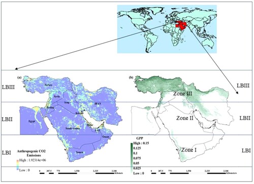
The Middle East region is located in the west of Asia and includes sixteen countries as Iran, Turkey, Egypt, Saudi Arabia, Iraq, Syria, Emirates, Kuwait, Qatar, Lebanon, Bahrain, Israel, Jordan, Oman, Palestine, and Yemen (Figure 1). The ME has a wild range of climate types but mainly arid and semi-arid with mild winter and low precipitation (Nandi, Bhattacharjee, and Chakraborty 2019). The population of ME is about 447.8 million, with an average of 1.65% population growth in 2020 (WDI 2021). Approximately more than 46% and 40% of the world's proven oil and gas reserves are located in the ME region, respectively (BP 2021), and more than 8% of the total world's anthropogenic CO₂ emissions are emitted from this area (Edgar 2020).

Figure 1. Spatial distribution of the annual mean of (a) ODIAC CO₂ emission and (b) GPP in ME from 2003 to 2019.

2.2. Datasets

2.2.1. OCO-2XCO₂ observations

NASA's OCO-2 is the first spacecraft devoted to CO₂ monitoring, which was successfully launched in July 2014 (Wunch et al. 2017). OCO-2 measures the CO₂ mole fraction in column-averaged dry air with the accuracy, resolution, and coverage needed to identify CO₂ sources and sinks on a regional and global scale (Crisp et al. 2004). This satellite operates in a Sun-synchronous orbit that flies at 705 km altitude with a local overpass time of 13:30 (Crisp et al. 2017). OCO-2 have a repeat cycle of 16 days and complete global XCO₂ coverage twice per month, with a spatial resolution of approximately 3 km². The validation results of OCO-2 data against high-precision measurements (ground-based or aircraft observations) indicate that precision is less than 0.5 ppm (Bi et al. 2018; Wang et al. 2021). In this research, the bias-corrected OCO-2 daily lite files (V10) from January 2015 to December 2020, with the quality flag as ‘0’ were utilized.

2.2.2. ODIAC CO₂ emissions

The monthly fossil fuel CO₂ emission from the open-source Data Inventory for Anthropogenic CO₂ (ODIAC) for January 2003 to December 2019 has been utilized to be compared with $\mathrm{\Delta }$XCO₂ variations. ODIAC is a monthly global anthropogenic CO₂ emission dataset based on estimates made by the Carbon Dioxide Information and Analysis Center (CDIAC) and satellite-observed nightlights and the power plant profile dataset, with a spatial resolution of 1 km × 1 km (Oda, Maksyutov, and Andres 2018). The climatology mean (CM) of annual ODIAC CO₂ emissions from 2003 to 2019 over ME is presented in Figure 1(a).

2.2.3. Vegetation absorption

Gross primary production (GPP) is a key measure of carbon mass flux in carbon cycle research, which is the total carbon fixation by terrestrial ecosystems through the photosynthesis of vegetation (Wang et al. 2012). In this study, GPP from Moderate-Resolution Imaging Spectroradiometer (MODIS; MOD17A2H) with a spatial resolution of 1 km × 1 km has been utilized as a parameter related to carbon uptake by vegetation photosynthesis (Figure 1b shows the CM of annual GPP in ME). The main vegetation cover in ME is observed in the west and north of Syria, Iran, and Iraq, along the Nile River in Egypt, and most parts of Turkey, with the maximum (minimum) average index in spring (winter).

2.3. Method

For extracting the CO₂ emission information from XCO₂, subtracting XCO_2-bg, to isolate the CO₂ source and sink signals, was considered based on the method described in Hakkarainen et al. (2019) study (Equation 1). The sensitivity of the method to the area for extracting medians, motivated the authors to calculate and compare the backgrounds in two different defined areas, the ME domain and the latitude bands (Figure 1). The day-to-day median from daily OCO-2XCO₂ in the ME domain was calculated in three zones with 10^◦ latitude widths from 11° to 22° (Zone I), 22° to 33° (Zone II) and 33° to 44° (Zone III), the daily median was also considered in three latitude bands from 11° to 22° (LB I), 22° to 33° (LB II) and 33° to 44° (LB III). The XCO_2-bg values in Zone I from 2015 to 2020 are presented in Figure 2. The XCO_2-bg in defined areas (ME domain and latitude bands) are compared in Section 3.1, and the daily $\mathrm{\Delta }$XCO₂ are then extracted from the individual XCO₂. Afterwards, the spatial daily $\mathrm{\Delta }$XCO₂ distribution maps with 0.25° × 0.25° grid cells were generated over ME using a space–time kriging prediction. The monthly, seasonal and annual $\mathrm{\Delta }$XCO₂ distribution maps to detect the spatial–temporal variations have been then extracted from daily maps. (1) $\mathrm{\Delta }\mathrm{XC}{\mathrm{O}}_2=\mathrm{XC}{\mathrm{O}}_2(\mathrm{individual})-\mathrm{XC}{\mathrm{O}}_2(\mathrm{dailybackground})$(1)

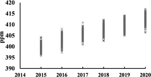
Figure 2. Daily XCO_2-bg in Zone I from 2015 to 2020.

The non-parametric Mann- Kendall trend test (MK) (Mann 1945; Kendall 1975) in analyzing time series trends and Mann–Whitney change point methods (MW) in detecting change points (CP) based on the differences in mean value (Ross 2015) are utilized for more detailed study in $\mathrm{\Delta }$XCO₂, GPP and ODIAC CO₂ emission time series. The assumption that the observations are independent (Von Storch and Zwiers 2001) is tested by the autocorrelation function (ACF) and if the time series of data are serially correlated, uncorrelated data is utilized by applying the pre-whitened data series (Shirvani, Arpe, and Jahandideh 2020). The autocorrelation function is the coefficient of correlation between two values in a time series, which describes the autocorrolation between an observation and the same observation at a prior time step (Box, Jenkins, and Reinsel 1994). Given measurements Y₁, Y₂, … , Y_N at time X₁, X₂, … , X_N, the lag k autocorrelation function with confidence bands of $(\pm 1.96/\sqrt{N})$ is defined as (Equation 2): (2) $rk={\displaystyle \frac{{\sum }_{i=1}^{N=k}(Y_i-\overline{Y})(Y_{i+k}-\overline{Y})}{{\sum }_{i=1}^N(Y_i-\overline{Y})}}$(2)

3. Results and discussions

3.1. XCO₂ backgrounds

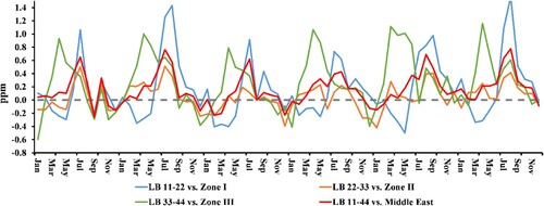
The time series of the monthly mean of CO_2-bg shows a strong seasonal cycle with an increasing trend (varying from 393 to 418 ppm) in all three zones as well as the whole ME domain and LBs (Figure 3). At the same time, the differences of CO_2-bg in ME (whole LB of 11° to 44°) from the CO_2-bg of study zones (LBs) were computed (Figures 4a and b). This comparison clearly shows the diversity in the CO_2-bg of Zone III against the other two zones, so that from April to September, the CO_2-bg shows fewer values than ME (positive values), and higher values in other months (negative values). However, Zone II shows a consistently higher CO_2-bg with the maximum values mostly in December and January and the minimum values in July and August. On the other hand, a similar comparison in LBs (Figure 4b) shows the same results, but with smoother fluctuations in LB II and LB III. In addition, the difference of the LBs CO_2-bg against the corresponding zones (Figure 5) shows that in general the LBs CO_2-bg have higher values than the corresponding zones. However, the graphs show an annual cycle with mostly positive values (referring to higher values of LBs CO_2-bg against the corresponding zones) especially in summertime (July and August) except for LB III vs. Zone III, which shows this maximum positive value almost in springtime (April and May). In addition, LB I vs. Zone I and then LB III vs. Zone III show the highest positive values particularly in August and April, respectively. However, the sharp negative values are seen in May in LB I vs. Zone I. Considering Figure 5 with the highest values in warm seasons (which is expected to have the lowest CO_2-bg based on Figure 3) and the lowest values in cold months (with the expectation of the highest CO_2-bg) or May in LB I vs. Zone I, guided the authors to believe the CO_2-bg which are extracted from the study zones can distinguish the sources of emission more clearly than the CO_2-bg in LBs. Thus, the further results will be based on the CO_2-bg values which are calculated over the three defined study zones. Furthermore, the sensitivity of CO_2-bg choice in local and regional studies is a critical step which is mentioned in previous studies in China or South Africa (Wang et al. 2018; Hakkarainen et al. 2019; Buchwitz et al. 2021; Fu et al. 2021).

Figure 3. Monthly mean of CO_2-bg in (a) the study zones and (b) the latitude bands.

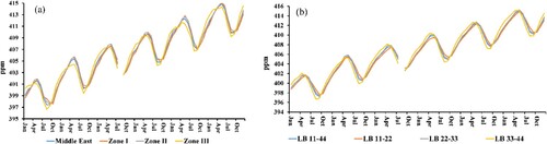
Figure 4. Monthly differences of CO_2-bg (a) zones vs. ME and (b) LBs vs. LB of 11°-44°.

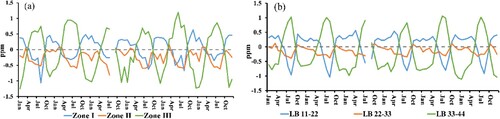
Figure 5. Monthly differences of CO_2-bg in LBs vs. the corresponding zones.

3.2. XCO₂ anomalies

For investigating the daily $\mathrm{\Delta }$XCO₂, the averages of daily $\mathrm{\Delta }$XCO₂ points were computed over the defined zones. The maximum and minimum in daily mean $\mathrm{\Delta }$XCO₂ shows both the most negative and positive values in Zone III for each month, while the fluctuations are the least in Zone II. The high fluctuation in Zone III can be explained by vegetation carbon sink (Figure 1b) and precipitation at especial periods which intensify the negative $\mathrm{\Delta }$XCO₂ values in Zone III, while large population, cold winter and utilizing heating systems and fossil fuels as well as industrial activities are the sources of CO₂ discharge. In addition, the maximum daily $\mathrm{\Delta }$XCO₂ values in Zones I and II are mostly recorded in cold months, while in Zone III the maximum $\mathrm{\Delta }$XCO₂ values are seen in both July and August as well as the cold months. Regarding the continuous days with relatively the highest $\mathrm{\Delta }$XCO₂ values in June, July or August in eastern Turkey and northwestern Iran in relation to high vegetation cover strengthens the possibility of biomass burning and its effect on high $\mathrm{\Delta }$XCO₂ values in the late springtime (June) and early/mid summertime (July and August). However, wildfire reports in 2015 and 2019 in northwestern to northeastern Iran and 2018–2020 in east, north and northeast Turkey emphasize this suspicion. In this regard, the importance of fire season in Africa is considered in $\mathrm{\Delta }$XCO₂ patterns in Hakkarainen et al. (2019) study. In addition, the westerly prevailing winds in this zone seem to play an important role in the general accumulation of carbon dioxide in the eastern regions of these countries. Nevertheless, in general the minimum $\mathrm{\Delta }$XCO₂ values are often seen in spring and summer.

In the following, the spatial mean in 0.25° × 0.25° grids as explained in Section 2.3 was considered for monthly, seasonal and annual periods. This leads to a spatial–temporal analysis of CO₂ sources and sinks over ME in defined periods as follows:

The CM of $\mathrm{\Delta }$XCO₂ for March and April as the months with approximately the most increase in vegetation cover show mostly the negative $\mathrm{\Delta }$XCO₂ values in eastern Iraq, Turkey, southern Oman and northern and northwestern Iran as well as Egypt, while the center and northeast of Iran as well as southern and southwestern of Saudi Arabia, show relatively positive $\mathrm{\Delta }$XCO₂ values (see Figure 6a for April). This is while in cold months by decreasing the role of photosynthesis and increasing the fossil fuel use, positive values are highlighted in Turkey and northwest Iran, however, Iraq and southwest Saudi Arabia, as well as southwest Iran, are the widest areas with constant positive $\mathrm{\Delta }$XCO₂ values during the year (see Figure 6b for December). These vast areas with constant positive $\mathrm{\Delta }$XCO₂ refer to the role of oil and gas extraction facilities as well as the role of megacities and the geopolitical situation of countries such as Iraq and Syria.

Figure 6. The CM for monthly $\mathrm{\Delta }$XCO₂ in 0.25° × 0.25° grids for (a) April and (b) December.

The CM for seasonal $\mathrm{\Delta }$XCO₂ shows the spatial displacement of positive and negative $\mathrm{\Delta }$XCO₂ values in different seasons, particularly in Turkey, western Iran, Iraq and Egypt. In this way, comparing the $\mathrm{\Delta }$XCO₂ in winter and spring shows a clear increase in the number of grids with positive anomalies in winter (Figure 7) for the mentioned areas. However, in Figure 8(a) the CM for annual $\mathrm{\Delta }$XCO₂ shows the highest values in Iraq as well as south regions of the Persian Gulf and south and southwest of Saudi Arabia, while despite the positive $\mathrm{\Delta }$XCO₂ values in Iran, generally less $\mathrm{\Delta }$XCO₂ values in comparison to the above mentioned areas are seen. At the same time, besides the areas with denser vegetation such as Turkey as well as north and northwest of Iran (Figure 1b), in the most defined periods, the minimum $\mathrm{\Delta }$XCO₂ or even the negative values are shown in Egypt, this is while by excluding the Nile Delta, the rest of the country is mostly classified as desert. However, more $\mathrm{\Delta }$XCO₂ values in Nile Delta in comparison to the surrounding desert go back to urbanization, dense population and irrigated farming which were mentioned in Shekhar et al. (2020) study. The latter reason refers to winter and summer as the peak of growing seasons which are receiving a high amount of carbon-rich water (Shekhar et al. 2020). This carbon-rich water will be then recycled and as a result causes CO₂ emission and thus higher $\mathrm{\Delta }$XCO₂ values in this region particularly in wintertime than in the surrounding desert (see Figure 7b). Recognizing the distinction in the Nile Delta emission by $\mathrm{\Delta }$XCO₂ in comparison to the surrounding area, as shown in Figures 6 and 7, clarifies the spatial capability and accuracy of the median method in determining the CO_2-bg and thus CO₂ emission, as resulted in Hakkarainen et al. (2019) study. However, the importance of CO₂ background choice in recognizing the local and regional emissions is mentioned in Buchwitz et al. (2021) study. In this regard, natural driving factors such as prevailing wind speed and direction as well as topography can be considered in a more detailed local investigation (Fu et al. 2021).

Figure 7. The CM for seasonal $\mathrm{\Delta }$XCO₂ from 2015 to 2020 for (a) spring and (b) winter in 0.25° × 0.25° grids.

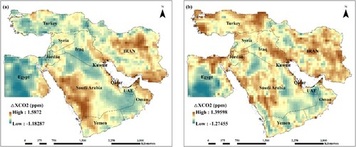
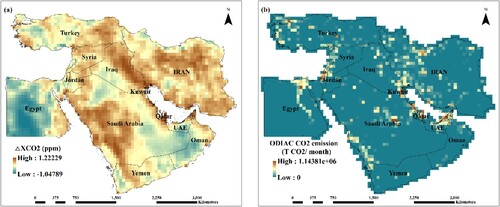
Figure 8. (a) The CM for annual $\mathrm{\Delta }$XCO₂ and (b) the CM for annual ODIAC CO₂ emission from 2015 to 2020 in 0.25° × 0.25° grids.

In the ME, deserts cover large areas including the Arabian Desert in Saudi Arabia, Dasht e Lut and Dasht e Kavir in the central part of Iran, which generally show less $\mathrm{\Delta }$XCO₂ values than the surrounding areas (Figures 6–8). However, in these countries, considering the significant role of wind (Fu et al. 2021), the transfer of CO₂ by the wind from major emission sources to surrounding areas reduces the $\mathrm{\Delta }$XCO₂ difference between deserts and the rest of the country.

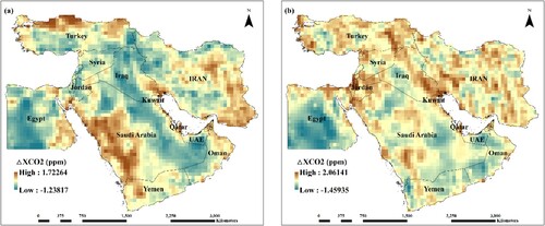
On the other hand, as a general effort to detect the changes in CO₂ emissions related to the COVID-19 pandemic, the $\mathrm{\Delta }$XCO₂ in March and April 2020 as the period with widespread lockdown were compared to the same month in the previous year. The results showed an increase in the number of pixels with less $\mathrm{\Delta }$XCO₂ values in March in comparison to the same month in 2019. In addition, for megacities such as Tehran, Istanbul, Ankara, Baghdad and Abu Dhabi in April 2020 relatively less $\mathrm{\Delta }$XCO₂ values were seen, compared to the same month in 2019 (Table 1). Figure 9 shows the $\mathrm{\Delta }$XCO₂ in March and April 2019 minus the same month of years 2020 and 2018. The negative values in Figures 9(a) and Figure 10(b) (March and April 2020 minus the same month of 2019) emphasize on $\mathrm{\Delta }$XCO₂ reductions while in the same comparison for 2019 and 2018, the general upward trend in CO₂ emission is dominant in major emission areas. Nevertheless, detailed information about the anthropogenic as well as natural CO₂ surface fluxes for more accurate and sophisticated analysis is suggested (Buchwitz et al. 2021).

Figure 9. The $\mathrm{\Delta }$XCO₂ difference in (a) March 2020 – March 2019 (b) April 2020 – April 2019 and for (c) March 2019 – March 2018 and (d) April 2019 – April 2018.

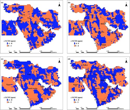
Figure 10. The monthly mean of GPP vs. the monthly total ODIAC CO₂ emission and monthly mean of $\mathrm{\Delta }$XCO₂ in Turkey.

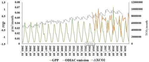
Table 1. The megacities $\mathrm{\Delta }$XCO₂ variation from 2015 to 2020 (ppm).

Megacities	2015	2016	2017	2018	2019	2020
Istanbul	0.921	0.373	1.149	0.057	0.799	0.714
Ankara	0.647	−0.774	0.187	0.240	1.520	0.917
Tehran	−0.723	−1.498	0.454	−0.337	0.478	−0.438
Riyadh	0.426	0.184	−0.159	−1.397	−0.493	1.382
Mecca	2.441	1.612	0.439	0.316	0.747	1.598
Doha	2.316	0.869	0.950	0.048	0.688	1.031
Abu Dhabi	−0.503	0.038	−0.881	−0.023	−0.028	−0.958
Baghdad	1.417	−0.812	0.954	−0.855	−1.432	−0.079

As described in the above paragraphs the combined effect of both human activities including the oil and gas industry, urbanization, population and transportation as well as natural features such as vegetation cover, is considerable and diagnostic in the spatial–temporal distribution of $\mathrm{\Delta }$XCO₂. So that in the following section, anthropogenic CO₂ emissions from ODIAC datasets and GPP is considered to further clarify the $\mathrm{\Delta }$XCO₂ variation in ME.

3.3. The $\mathrm{\Delta }$XCO₂ interaction with natural and anthropogenic driving factors

The CM for annual $\mathrm{\Delta }$XCO₂ (Figure 8a) comparison with the CM for annual anthropogenic CO₂ emission from the ODIAC dataset (Figure 8b) in the study period shows acceptable coordination between the regions with relatively the highest $\mathrm{\Delta }$XCO₂ values and the corresponding pixels with the highest anthropogenic emissions. On the other hand, the inter-annual $\mathrm{\Delta }$XCO₂ fluctuations over ME (Figures 6 and 7) particularly in Turkey, the Nile Delta region, the east of Iraq and the north and northwestern Iran emphasize on natural driving factors. In this way, the time series of monthly total ODIAC CO₂ emission, as well as the monthly mean of GPP in Saudi Arabia, Iran, Iraq, Turkey, Egypt and the regions of Syria, Lebanon, Israel and Palestine (as the countries with a complex interaction of geopolitical situations, oil and gas industry or vegetation cover), were extracted to compare the natural and anthropogenic driving factors against $\mathrm{\Delta }$XCO₂ fluctuations. In general, no significant trend is detected in $\mathrm{\Delta }$XCO₂ and GPP in mentioned countries as well as the whole ME area based on the MK test, while the ODIAC CO₂ emission shows a general upward trend. At the same time, the inverse relationship between $\mathrm{\Delta }$XCO₂ and ODIAC CO₂ emission with GPP is mostly observed in Turkey, Iran, Iraq and the regions of Syria, Lebanon, Israel and Palestine, while no clear inverse relationship is considered in Saudi Arabia and Egypt (with poor vegetation cover) particularly in GPP and ODIAC CO₂ emission comparison. However, a general one to two months lag is seen in a monthly maximum of GPP values versus monthly minimum values of $\mathrm{\Delta }$XCO₂ and ODIAC CO₂ emission (see Figure 10 for Turkey).

The ODIAC CO₂ emission seems to show two breaks in the general upward trend of Saudi Arabia in January 2007 and January 2016 respectively (Figure 11(. The monthly total ODIAC CO₂ emission versus the monthly mean of $\mathrm{\Delta }$XCO₂ and monthly mean of GPP for Saudi Arabia are shown in Figures 12(a and b), respectively. The short period in $\mathrm{\Delta }$XCO₂ values (available since 2015) in Figure 13(a), does not provide sufficient evidence in explaining these sharp changes. On the other hand, in Figure 12(b) despite the equal period of two datasets, the GPP time series with no significant upward nor downward trend does not explain the ODIAC CO₂ emission breaks. Accordingly, the proceedings such as pollutant filtering of oil and gas extraction industry, improving the public transportation, and changes in cooling facilities as well as planning to plant trees, probably is the reason for changes in ODIAC CO₂ emission changes since 2016. However, what is relevant to the present study is the insufficient length of $\mathrm{\Delta }$XCO₂ in justifying the changes in the anthropogenic CO₂ emission in Saudi Arabia. At the same time, CP detection in $\mathrm{\Delta }$XCO₂, GPP and ODIAC CO₂ emission time series are considered in ME as well as the mentioned countries. The ODIAC CO₂ emission shows the only significant CP in December 2015 for Saudi Arabia and January 2016 for ME. This is while the CP in GPP was detected only in Saudi Arabia (October 2015), and no significant CP in $\mathrm{\Delta }$XCO₂ was detected in studied countries as well as the whole ME area. The almost simultaneous CP in ME and Saudi Arabia for ODIAC CO₂ emission can refer to the significant and critical role of some industrial regions or countries in anthropogenic CO₂ emission, however, no significant upward nor downward trend in $\mathrm{\Delta }$XCO₂ emphasizes on an overall moderating effect of some driving factors against the intensifying effect of other factors in CO₂ emission.

Figure 11. The monthly total ODIAC CO₂ emission in some selected countries in ME.

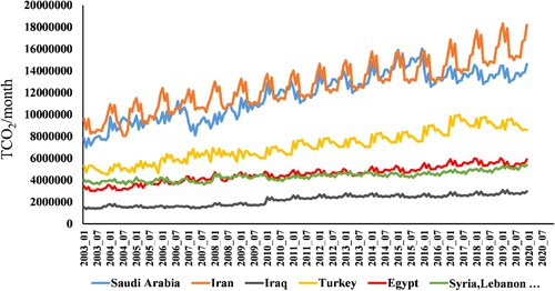
Figure 12. The monthly total ODIAC CO₂ emission vs. (a) $\mathrm{\Delta }$XCO₂ and (b) GPP in Saudi Arabia.

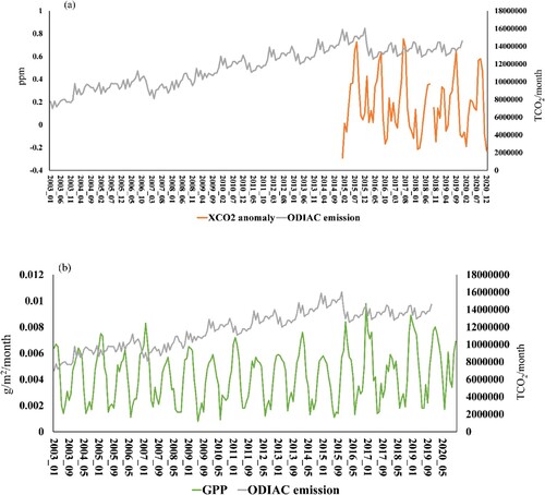
Figure 13. The six selected polygons in ME.

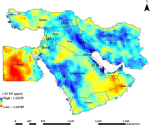
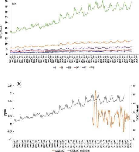
However, for a more detailed study the regions with relatively the highest $\mathrm{\Delta }$XCO₂ values (corresponded with the highest ODIAC CO₂ emissions (Figure 8)) were considered as individual polygons independent of political boundaries. Figure 13 shows the approximate location of selected polygons which are named Polygon I to VI. The time series of the monthly mean of CO₂ emissions from the ODIAC dataset is presented in Figure 14(a), which shows the highest level of the monthly mean of ODIAC CO₂ emission in Polygon VI (the southern margin of the Persian Gulf and Oman Sea). In this polygon, despite the small portion of the area in ME and as a result the lower total emissions, the monthly mean of CO₂ emissions show a clear higher value than other polygons. In addition, in ODIAC CO₂ emissions the only CP was detected in January 2015 in Polygon VI, while $\mathrm{\Delta }$XCO₂ shows sharp fluctuations in this polygon (Figure 14b). This confirms the capability of $\mathrm{\Delta }$XCO₂ values to detect the regions with high emissions and as a result detect the carbon cycle which is contributed to perturbation in CO₂ concentrations.

Figure 14. (a) The monthly mean of CO₂ Emission from ODIAC in 6 selected polygons and (b) ODIAC CO₂ emission vs. $\mathrm{\Delta }$XCO₂ in polygon VI.

4. Conclusions

In our study using 6 years of OCO-2XCO₂ product, the XCO₂ anomalies over the Middle East were computed based on the daily medians in each defined zones. The daily $\mathrm{\Delta }$XCO₂ values varied in the range of −4–5.5 ppm which were smoothed in monthly, seasonal or yearly time scales. The results showed the capability of space-based observation and as a result $\mathrm{\Delta }$XCO₂ in spatial and temporal analysis of regional CO₂ sources and sinks, including mainly the anthropogenic CO₂ emission as well as biomass burning and vegetation absorption.

The $\mathrm{\Delta }$XCO₂ variation pattern over ME detected the anthropogenic CO₂ emission mainly in areas with the oil and gas industry as well as populated areas and megacities. Furthermore, biomass burning in some regions of Turkey and Iran was detectible in months with high vegetation cover along with high air temperature and arid situation. In addition, the reduction in CO₂ emission during widespread lockdown in March and April 2020 was recognized in densely populated cities such as Tehran, Istanbul, Ankara, Baghdad and Abu Dhabi based on the $\mathrm{\Delta }$XCO₂ comparison with the same months in 2019. The impact of biomass absorption and photosynthesis activity as CO₂ sinks are highlighted in seasonal patterns of $\mathrm{\Delta }$XCO₂, particularly in Zone III with higher vegetation cover. In this regard, small countries such as Qatar and the United Arab Emirates or large countries with relatively small populations such as Saudi Arabia are recognized as the regions with constant and high $\mathrm{\Delta }$XCO₂ values, while the Nile Delta region, Turkey, north and northwestern Iran, and some parts of Iraq with high vegetation cover show more seasonal fluctuations in CO₂ anomalies.

The high consistency between $\mathrm{\Delta }$XCO₂ variation patterns and ODIAC as well as GPP datasets as fossil fuel CO₂ emission and biospheric contribution emphasizes on the spatial–temporal capability of the CO₂ anomaly method for detecting anthropogenic CO₂ emission patterns. However, according to the regional variation patterns of $\mathrm{\Delta }$XCO₂ and regional driving factors, additional study considering wind patterns along with topography is suggested.

Data availability statement

The data that support the findings of this study are available from the corresponding author upon reasonable request.

Acknowledgements

The authors thank the open sources data, the NASA Goddard Earth Science Data and Information Services Center for providing OCO-2 data products, the NASA Land Processes Distributed Active Archive Center (LP DAAC) for providing MODIS data products, and the National Institute for Environment Studies (NIES) for providing support to ODIAC.

Disclosure statement

No potential conflict of interest was reported by the author(s).

References

- Ahlström, A., M. R. Raupach, G. Schurgers, B. Smith, A. Arneth, M. Jung, and N. Zeng. 2015. “The Dominant Role of Semi-Arid Ecosystems in the Trend and Variability of the Land CO2 Sink.” Science 348 (6237): 895–899.
- Bi, Y., Q. Wang, Z. Yang, J. Chen, and W. Bai. 2018. “Validation of Column-Averaged Dry-Air Mole Fraction of CO2 Retrieved from OCO-2 Using Ground-Based FTS Measurements.” Journal of Meteorological Research 32 (3): 433–443.
- Bovensmann, H., M. Buchwitz, J. P. Burrows, M. Reuter, T. Krings, K. Gerilowski, and J. Erzinger. 2010. “A Remote Sensing Technique for Global Monitoring of Power Plant CO2 Emissions from Space and Related Applications.” Atmospheric Measurement Techniques 3 (4): 781–811.
- Box, G. E. P., G. M. Jenkins, and G. C. Reinsel. 1994. Time Series Analysis; Forecasting and Control. 3rd ed. Englewood Cliff: Prentice Hall.
- BP. 2021. “Statistical Review of World Energy 2021.” Accessed March 22, 2021 https://www.bp.com/en/global/corporate/energy-economics/statistical-review-ofworld-energy.html.
- Buchwitz, M., M. Reuter, S. Noël, K. Bramstedt, O. Schneising, M. Hilker, and D. Crisp. 2021. “Can a Regional-Scale Reduction of Atmospheric CO2 During the COVID-19 Pandemic be Detected from Space? A Case Study for East China Using Satellite XCO2 Retrievals.” Atmospheric Measurement Techniques 14 (3): 2141–2166.
- Crisp, D., R. M. Atlas, F. M. Breon, L. R. Brown, J. P. Burrows, P. Ciais, and C. E. Miller. 2004. “The Orbiting Carbon Observatory (OCO) Mission.” Advances in Space Research 34 (4): 700–709.
- Crisp, D., H. R. Pollock, R. Rosenberg, L. Chapsky, R. A. Lee, F. A. Oyafuso, and D. Wunch. 2017. “The on-Orbit Performance of the Orbiting Carbon Observatory-2 (OCO-2) Instrument and its Radiometrically Calibrated Products.” Atmospheric Measurement Techniques 10 (1): 59–81.
- Edgar. 2020. Accessed April 18, 2020. website: https://edgar.jrc.ec.europa.eu/overview.php?v = booklet2019.
- Falahatkar, S., S. M. Mousavi, and M. Farajzadeh. 2017. “Spatial and Temporal Distribution of Carbon Dioxide gas Using GOSAT Data Over IRAN.” Environmental Monitoring and Assessment 189 (12): 1–13.
- Fu, Y., W. Sun, F. Luo, Y. Zhang, and X. Zhang. 2021. “Variation Patterns and Driving Factors of Regional Atmospheric CO2 Anomalies in China.” Environmental Science and Pollution Research 29 (13): 19390–19403.
- Gavrilov, N. M., M. V. Makarova, A. V. Poberovskii, and Y. M. Timofeyev. 2014. “Comparisons of CH4 Ground-Based FTIR Measurements Near Saint Petersburg with GOSAT Observations.” Atmospheric Measurement Techniques 7 (4): 1003–1010.
- Gloudemans, A. M. S., M. C. Krol, J. F. Meirink, A. T. J. De Laat, G. R. Van der Werf, H. Schrijver, and I. Aben. 2006. “Evidence for Long-Range Transport of Carbon Monoxide in the Southern Hemisphere from SCIAMACHY Observations.” Geophysical Research Letters 33 (16): 1–5.
- Golkar, F., M. Al-Wardy, S. F. Saffari, K. Al-Aufi, and G. Al-Rawas. 2020. “Using OCO-2 Satellite Data for Investigating the Variability of Atmospheric CO2 Concentration in Relationship with Precipitation, Relative Humidity, and Vegetation Over Oman.” Water 12 (1): 101.
- Golkar, F., and A. Shirvani. 2020. “Spatial and Temporal Distribution and Seasonal Prediction of Satellite Measurement of CO2 Concentration Over Iran.” International Journal of Remote Sensing 41 (23): 8891–8909.
- Hakkarainen, J., I. Ialongo, S. Maksyutov, and D. Crisp. 2019. “Analysis of Four Years of Global XCO2 Anomalies as Seen by Orbiting Carbon Observatory-2.” Remote Sensing 11 (7): 850.
- Hakkarainen, J., I. Ialongo, and J. Tamminen. 2016. “Direct Space-Based Observations of Anthropogenic CO2 Emission Areas from OCO-2.” Geophysical Research Letters 43 (21): 11–400.
- He, Z., L. Lei, L. Welp, Z. Zeng, N. Bie, S. Yang, and L. Liu. 2018. “Detection of Spatiotemporal Extreme Changes in Atmospheric CO2 Concentration Based on Satellite Observations.” Remote Sens-Basel 10: 839. doi:10.3390/rs10060839.
- He, Z., L. Lei, Y. Zhang, M. Sheng, C. Wu, L. Li, and L. R. Welp. 2020. “Spatio-temporal Mapping of Multi-Satellite Observed Column Atmospheric CO2 Using Precision-Weighted Kriging Method.” Remote Sensing 12 (3): 576.
- Houweling, S., W. Hartmann, I. Aben, H. Schrijver, J. Skidmore, G. J. Roelofs, and F. M. Breon. 2005. “Evidence of Systematic Errors in SCIAMACHY-Observed CO2 due to Aerosols.” Atmospheric Chemistry and Physics 5 (11): 3003–3013.
- IPCC. 2014. “Climate Change 2014: Mitigation of Climate Change. Contribution of Working Group III to the Fifth Assessment Report of the Intergovernmental Panel on Climate Change.” In Edenhofer, O., R. Pichs-Madruga, Y. Sokona, E. Farahani, S. Kadner, K. Seyboth, A. Adler, I. Baum, S. Brunner, P. Eickemeier, B. Kriemann, J. Savolainen, S. Schlömer, C. von Stechow, T. Zwickel and J.C. Minx (eds.) Cambridge University Press, Cambridge. ISAAKS, E.H.; SRIVASTAVA R. M., An Introduction to Applied Geostatistics. Nova Iorque, Oxford University, 1989.
- Ishizawa, M., K. Mabuchi, T. Shirai, M. Inoue, I. Morino, O. Uchino, and S. Maksyutov. 2016. “Inter-annual Variability of Summertime CO2 Exchange in Northern Eurasia Inferred from GOSAT XCO2.” Environmental Research Letters 11 (10): 105001.
- Janardanan, R., S. Maksyutov, T. Oda, M. Saito, J. W. Kaiser, A. Ganshin, and T. Yokota. 2016. “Comparing GOSAT Observations of Localized CO2 Enhancements by Large Emitters with Inventory-Based Estimates.” Geophysical Research Letters 43 (7): 3486–3493.
- Kendall, M. G. 1975. Rank Correlation Methods. 4th ed, 272. London, UK: Charles Griffin.
- Kiel, M., C. W. O'Dell, B. Fisher, A. Eldering, R. Nassar, C. G. MacDonald, and P. O. Wennberg. 2019. “How Bias Correction Goes Wrong: Measurement of X CO 2 Affected by Erroneous Surface Pressure Estimates.” Atmospheric Measurement Techniques 12 (4): 2241–2259.
- Kort, E. A., C. Frankenberg, C. E. Miller, and T. Oda. 2012. “Space-Based Observations of Megacity Carbon Dioxide.” Geophysical Research Letters 39: 17.
- Kountouris, P., C. Gerbig, C. Rödenbeck, U. Karstens, T. F. Koch, and M. Heimann. 2018. “Atmospheric CO2 Inversions on the Mesoscale Using Data-Driven Prior Uncertainties: Quantification of the European Terrestrial CO2 Fluxes.” Atmospheric Chemistry and Physics 18 (4): 3047–3064.
- Kumar, M. K., and S. S. Nagendra. 2016. “Quantification of Anthropogenic CO2 Emissions in a Tropical Urban Environment.” Atmospheric Environment 125: 272–282.
- Mann, H. B. 1945. “Nonparametric Tests Against Trend.” Econometrica 13: 245–259.
- Mousavi, S. M., N. M. Dinan, S. Ansarifard, and O. Sonnentag. 2022. “Analyzing Spatio-Temporal Patterns in Atmospheric Carbon Dioxide Concentration Across Iran from 2003 to 2020.” Atmospheric Environment: X 14: 100163.
- Mousavi, S. M., and S. Falahatkar. 2020. “Spatiotemporal Distribution Patterns of Atmospheric Methane Using GOSAT Data in Iran.” Environment, Development and Sustainability 22 (5): 4191–4207.
- Mousavi, S. M., S. Falahatkar, and M. Farajzadeh. 2017. “Assessment of Seasonal Variations of Carbon Dioxide Concentration in I Ran Using GOSAT Data.” Natural Resources Forum 41 (2): 83–91.
- Nandi, C., S. Bhattacharjee, and S. Chakraborty. 2019. “Climate Change and Energy Dynamics with Solutions: A Case Study in Egypt.” In Climate Change and Energy Dynamics in the Middle East, 225–257. Cham: Springer.
- Nassar, R., T. G. Hill, C. A. McLinden, D. Wunch, D. B. Jones, and D. Crisp. 2017. “Quantifying CO2 Emissions from Individual Power Plants from Space.” Geophysical Research Letters 44 (19): 10–045.
- Nguyen, H., G. Osterman, D. Wunch, C. O'Dell, L. Mandrake, P. Wennberg, and R. Castano. 2014. “A Method for Colocating Satellite XCO2 Data to Ground-Based Data and its Application to ACOS-GOSAT and TCCON.” Atmospheric Measurement Techniques 7 (8): 2631–2644.
- Oda, T., S. Maksyutov, and R. J. Andres. 2018. “The Open-Source Data Inventory for Anthropogenic CO2, Version 2016 (ODIAC2016): A Global Monthly Fossil Fuel CO2 Gridded Emissions Data Product for Tracer Transport Simulations and Surface Flux Inversions.” Earth System Science Data 10 (1): 87–107.
- Pan, G., Y. Xu, and J. Ma. 2021. “The Potential of CO2 Satellite Monitoring for Climate Governance: A Review.” Journal of Environmental Management 277: 111423.
- Reuter, M., M. Buchwitz, A. Hilboll, A. Richter, O. Schneising, M. Hilker, and J. P. Burrows. 2014. “Decreasing Emissions of NO x Relative to CO2 in East Asia Inferred from Satellite Observations.” Nature Geoscience 7 (11): 792–795.
- Reuter, M., M. Buchwitz, O. Schneising, S. Noël, H. Bovensmann, J. P. Burrows, and D. Schepers. 2020. “Ensemble-based Satellite-Derived Carbon Dioxide and Methane Column-Averaged dry-air Mole Fraction Data Sets (2003–2018) for Carbon and Climate Applications.” Atmospheric Measurement Techniques 13 (2): 789–819.
- Ross, G. J. 2015. “Parametric and Nonparametric Sequential Change Detection in R: The cpm Package.” Journal of Statistical Software 66: 1–20.
- Schwandner, F. M., M. R. Gunson, C. E. Miller, S. A. Carn, A. Eldering, T. Krings, and J. R. Podolske. 2017. “Spaceborne Detection of Localized Carbon Dioxide Sources.” Science 358 (6360): eaam5782.
- Shekhar, A., J. Chen, J. C. Paetzold, F. Dietrich, X. Zhao, S. Bhattacharjee, and S. C. Wofsy. 2020. “Anthropogenic CO2 Emissions Assessment of Nile Delta Using XCO2 and SIF Data from OCO-2 Satellite.” Environmental Research Letters 15 (9): 095010.
- Shi, K., B. Yu, Y. Zhou, Y. Chen, C. Yang, Z. Chen, and J. Wu. 2019. “Spatiotemporal Variations of CO2 Emissions and Their Impact Factors in China: A Comparative Analysis Between the Provincial and Prefectural Levels.” Appl Energ 233–234: 170–181. doi:10.1016/j.apenergy.2018.10.050.
- Shirvani, A., A. Arpe, and M. Jahandideh. 2020. “Analysis of Trends and Change Points in Meteorological Variables Over the South of the Caspian Sea.” Theoretical and Applied Climatology 141: 959–966.
- Von Storch, H., and F. W. Zwiers. 2001. Statistical Analysis in Climate Research. Cambridge: Cambridge university press.
- Wang, X., M. Ma, G. Huang, F. Veroustraete, Z. Zhang, Y. Song, and J. Tan. 2012. “Vegetation Primary Production Estimation at Maize and Alpine Meadow Over the Heihe River Basin, China.” International Journal of Applied Earth Observation and Geoinformation 17: 94–101.
- Wang, Q., F. Mustafa, L. Bu, S. Zhu, J. Liu, and W. Chen. 2021. “Atmospheric Carbon Dioxide Measurement from Aircraft and Comparison with OCO-2 and Carbon Tracker Model Data.” Atmospheric Measurement Techniques 14 (10): 6601–6617.
- Wang, S., Y. Zhang, J. Hakkarainen, W. Ju, Y. Liu, F. Jiang, and W. He. 2018. “Distinguishing Anthropogenic CO2 Emissions from Different Energy Intensive Industrial Sources Using OCO-2 Observations: A Case Study in Northern China.” J. Geophys. Res. Atmos 123: 9462–9473.
- WDI. 2021. “World Development Indicators Databank.” Accessed May 13, 2021. https://databank.worldbank.org/-home.aspx#advancedDownloadOptions.
- Wu, D., J. C. Lin, B. Fasoli, T. Oda, X. Ye, T. Lauvaux, and E. A. Kort. 2018. “A Lagrangian Approach Towards Extracting Signals of Urban CO 2 Emissions from Satellite Observations of Atmospheric Column CO2 (XCO 2): X-Stochastic Time-Inverted Lagrangian Transport Model (“X-STILT v1”).” Geoscientific Model Development 11 (12): 4843–4871.
- Wunch, D., P. O. Wennberg, G. Osterman, B. Fisher, B. Naylor, C. M. Roehl, and A. Eldering. 2017. “Comparisons of the Orbiting Carbon Observatory-2 (OCO-2) XCO2 Measurements with TCCON.” Atmospheric Measurement Techniques 10 (6): 2209–2238.
- Yang, E. G., E. A. Kort, D. Wu, J. C. Lin, T. Oda, X. Ye, and T. Lauvaux. 2020. “Using Space-Based Observations and Lagrangian Modeling to Evaluate Urban Carbon Dioxide Emissions in the Middle East.” Journal of Geophysical Research: Atmospheres 125 (7): 1–20. doi:10.1029/2019JD031922.
- Yokota, T., Y. Yoshida, N. Eguchi, Y. Ota, T. Tanaka, H. Watanabe, and S. Maksyutov. 2009. “Global Concentrations of CO2 and CH4 Retrieved from GOSAT: First Preliminary Results.” Sola 5: 160–163.
- Yoshida, Y., N. Kikuchi, I. Morino, O. Uchino, S. Oshchepkov, A. Bril, and T. Yokota. 2013. “Improvement of the Retrieval Algorithm for GOSAT SWIR XCO 2 and XCH 4 and Their Validation Using TCCON Data.” Atmospheric Measurement Techniques 6 (6): 1533–1547.
- Zheng, B., F. Chevallier, P. Ciais, G. Broquet, Y. Wang, J. Lian, and Y. Zhao. 2020. “Observing Carbon Dioxide Emissions Over China's Cities and Industrial Areas with the Orbiting Carbon Observatory-2.” Atmospheric Chemistry and Physics 20 (14): 8501–8510.