An effective global learning framework for hyperspectral image classification based on encoder-decoder architecture

ABSTRACT

Most deep learning methods in hyperspectral image (HSI) classification use local learning methods, where overlapping areas between pixels can lead to spatial redundancy and higher computational cost. This paper proposes an efficient global learning (EGL) framework for HSI classification. The EGL framework was composed of universal global random stratification (UGSS) sampling strategy and a classification model BrsNet. The UGSS sampling strategy was used to solve the problem of insufficient gradient variance resulted from limited training samples. To fully extract and explore the most distinguishing feature representation, we used the modified linear bottleneck structure with spectral attention as a part of the BrsNet network to extract spectral spatial information. As a type of spectral attention, the shuffle spectral attention module screened important spectral features from the rich spectral information of HSI to improve the classification accuracy of the model. Meanwhile, we also designed a double branch structure in BrsNet that extracted more abundant spatial information from local and global perspectives to increase the performance of our classification framework. Experiments were conducted on three famous datasets, IP, PU, and SA. Compared with other classification methods, our proposed method produced competitive results in training time, while having a greater advantage in test time.

KEYWORDS:

• Deep learning
• global learning
• feature representation
• hyperspectral image classification
• spectral attention

1. Introduction

The high dimensionality of hyperspectral image (HSI) enables them to identify the subtle differences in spectral dimensions of different ground objects. For this reason, HSI has been widely used in agriculture (Teke et al. 2013), forestry management (Coops et al. 2003), water and marine resource management (Younos and Parece 2015), geological exploration and mineralogy (Resmini et al. 1997), and urban planning (Abbate et al. 2003). In these applications, hyperspectral image classification plays a very important role. HSI classification aims to assign a unique semantic label to each pixel in a hyperspectral image, which is a fundamental but challenging work for the hyperspectral images.

In the early days of HSI classification, multiple methods were proposed to tap the potential of rich spectral information from HSI in hyperspectral image classification. The methods, such as neural network (Fu, Ma, and Wang 2018), support vector machine (SVM) (Wang and Feng 2008), multinomial logistic regression (Li, Bioucas-Dias, and Plaza 2010) and other relevant methods, have been successfully used for HSI classification. Meanwhile, due to the Hughes phenomenon in hyperspectral images (Hughes 1968) that greatly limits the ability of HIS classification, some researchers have focused on designing dimensionality reduction techniques, such as principal component analysis (PCA) (Deepa and Thilagavathi 2015; Imani and Ghassemian 2014), independent component analysis (ICA) (Jayaprakash et al. 2018; Wang and Chang 2006) and the Linear Discriminant Approach (LDA) (Du 2007). Recently, a collaborative and low-rank graph for discriminant analysis (CLGDA) was developed for HSI dimensionality reduction (Shah and Du 2021). Subsequently, a novel collaborative representation-based graph embedding method was proposed by the same group (Shah and Du 2022). This method further improves the performance as it allows spatial neighbors to make more contributions to the representation. However, the performance of these methods is usually unsatisfactory, because the dimensionality reduction of these methods will lose much of the rich spectral information of HSI leading to suboptimal results. As the HIS often appears in ‘synonyms spectrum’ and ‘foreign body with the spectrum’ of the phenomenon, good classification results cannot be achieved just relying on spectral information. To address this problem, Yan et al. (2010) proposed a classification method that combined the spatial information with spectral information to avoid the abovementioned phenomenon, which improved the classification accuracy. Since then, more methods have been focused on the spatial information of HSI, especially on the extraction of spatial information including the extended morphological contour method (Wang et al. 2016; Zhang, sun, and Qi 2018) and the joint sparse representation model (Fang et al. 2014). Based on spatial spectral information, these classification methods have demonstrated improved results. However, most of them were designed for specific application scenarios and their performance is limited if applied to other scenarios. For example, These methods often adopt hand-crafted features designed by experts. However, these hand-crafted features may not be sufficient to distinguish slightly different objects. Thus, how to automatically and accurately extract more discriminant features is still the key to model performance in HSI classification.

To address this issue, deep learning technique has been introduced into HSI classification. Compared with traditional feature extraction method, CNN-based deep learning methods can automatically learn discriminant features, and their end-to-end characteristics enable their feature extractors and classifiers to be globally optimized for better accuracy. Most CNN-based methods adopt the patch-based local learning framework, which can extract the neighborhood elements of the pixel to form the neighborhood pixel block as the input of the classification model. In this case, the type of the central pixel is determined by the type of each pixel in the neighborhood pixel block. However, due to the large number of overlapping regions of adjacent patches, the patch-based methods often increase the computational complexity, and cannot sufficiently utilize spatial information.

In order to solve the problems in patch-based learning framework, Zheng et al. (2020) proposed a fast patchless global learning (FPGA) framework, which maximizes the use of global spatial information through the combination of sampling strategy and classification model. The FPGA framework decreases redundant computation and achieves high classification accuracy on three public datasets. However, when a dataset has a small scale of sampling data, the sampling method in FPGA is difficult to guarantee its universality.

This paper proposed an efficient global learning framework which includes a Universal Global Stochastic Stratified (UGSS) sampling strategy and a classification networkcalled BrsNet based on encoder-decoder structure of Deeplabv3+ (Chen et al. 2018). Compared with the sampling strategy of FPGA, the proposed UGSS sampling strategy can obtain sufficient hierarchical data in a small sample data set to ensure the normal training and convergence of the classification model. The BrsNet framework aims to fully exploit spatial information to further improve performance. The encoder part of BrsNet consists of a modified linear bottleneck structure with spectral attention (MLBSA) and a double branch structure. The decoder part is a lightweight structure that includes shuffle spectral attention (SSA) module to improve the effectiveness of the model. In addition, the encoder-decoder structure of BrsNet has a better effect on the restoration of image edge.

The main contributions of this paper are summarized as follows:

1. An effective global learning (EGL) framework is proposed for HSI classification. EGL includes the UGSS sampling strategy and the encoder-decoder structure-based classification network BrsNet;

2. The UGSS sampling strategy is designed for the model training to ensure the convergence of model training as well as the stability and effectiveness of the framework in some small sample data sets. The UGSS sampling strategy generates random layered training sample data to obtain more gradients in the back propagation of the model. Then, the layered adjustment operation is also carried out based on the sample size, so that UGSS sampling strategy can be applied to datasets with less sample data;

3. A network structure BrsNet for HSI classification using global spatial information is proposed. The BrsNet is an encoder-decoder structure network based on deeplabv3+. BrsNet consists of the modified linear bottleneck structure with spectral attention, a bi-branch structure with atrous spatial pyramid pooling (ASPP) (Chen et al. 2017) and Criss-Cross Attention (CCA) module (Huang et al. 2019), which can extract spatial information from global and multi-scale local information respectively;

4. We improve the traditional Sequeze and Excitation (SEBlock) spectral attention mechanism and design a shuffle spectral attention module. SSA can improve the interaction between channels, intensify the spectral features with rich information and suppress the spectral features with less information.

2. Related works

In this section, we briefly introduce the related work involved in our proposed method to illustrate the current state of HSI classification development, the development of semantic segmentation models and their relevance to HSI classification. Finally, we describe the explanation of the attention mechanism.

2.1 HSI classification

HSI classification has been widely studied due to the importance in HSI processing. A variety of methods for HSI classification have been proposed, including traditional logistic regression (Li, Bioucas-Dias, and Plaza 2012), SVM (Wang and Feng 2008), ELM (Su, Cai, and Du 2017), and sparse representation (Yu et al. 2020). Although these methods have achieved certain results, they were not designed to combine the rich spectral and spatial information of HSI, which could potentially produce better results. Additionally, the empirically-based feature extraction from previous methods often performs poorly in describing the essential properties of hyperspectral data.

To obtain better classification results, deep learning models such as stacked autoencoders, deep belief networks, convolutional neural networks (CNN), recurrent neural networks, and generative adversarial networks have been developed for HSI classification. In consideration of CNN-based methods having obvious advantages in HSI classification, Zhong et al. (2017) designed a spectral and spatial residual block to continuously learn discriminative features from the rich spectral features and spatial context in HSI, and proposed a spectral-spatial residual network. Wang et al. (2018a) use different convolution kernel sizes to extract spectral and spatial features separately, and use valid convolution to reduce high dimensionality. Li et al. (2020) designed two branches to capture spectral information and spatial information, respectively, to refine and optimize the feature maps extracted by the network. Hong et al. (2022) designed a transformer-based network architecture capable of learning local spectral representations from multiple adjacent bands instead of a single band at each encoding position, thereby improving the accuracy of HSI classification. Many existing deep model methods are patch-based. Although these patch-based methods have greatly improved accuracy in HSI classification, the redundant computation of overlapping regions of these methods still poses new challenges. To some extent, the redundant computation generated by these methods has limited the further development of HSI classifiers.

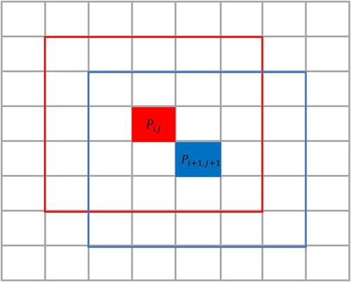
Figure 1 shows the overlapping pixels generated by a patch-based learning method. The pixel fields centered on the red and blue regions have many repeating pixels as these pixels are fields of multiple center pixels. Although this patch-based method has improved accuracy, they cannot avoid redundant computation between adjacent shards. The input of the classification method of this model is the neighborhood pixel block. The label of the neighborhood pixel block is determined by the label of the central pixel, which can improve the accuracy by using the spatial information of the neighborhood pixel block.

Figure 1. The patch-based learning method has a large number of repeated pixels, where $P_{ij}$ and $P_{i+1,j+1}$ are their center pixels, respectively.

In order to minimize the computational redundancy caused by spatial overlap and reduce the loss of spatial information, researchers have developed classification methods based on fully convolutional network (FCN) (Long, Shelhamer, and Darrell 2015). FCN take the entire HSI as the input of the model and generating the corresponding class map, which reduces the computational redundancy and improves the classification performance. The DMS3FE classifier (Jiao et al. 2017) uses a pretrained FCN to extract features, but the FCN is not trained. Shen et al. (2020) designed an FCN without downsampling, where the input and output feature maps are of the same size, but for some datasets, it does not directly use global spatial information for classification. Both methods only use FCN to extract features, and the global spatial information has not been fully utilized.

To solve the problem of model convergence and mine the global spatial context information, Zheng et al. (2020) proposed an FPGA framework, which is a deep convolutional model based on encoder-decoder architecture. FPGA introduces a global stochastic hierarchical GS² sampling strategy to obtain different gradients to guarantee the convergence of classification model in FPGA. GS² sampling strategy takes the whole HSI as the input of the classification model, which effectively avoids the redundancy of the patch-based sampling strategy.

2.2 Models based on semantic segmentation tasks

In the CNN segmentation model, there is often a convolutional layer or a pooling layer with a stride greater than 1 for downsampling to extract more abstract features. The dimension of the feature map obtained at this time will be reduced, and more advanced features and richer semantic information will be obtained, which is suitable for common classification tasks only predicting global probabilities. For semantic segmentation, the classification probability of different positions of the image needs to be given. If the feature map is too small, much of the information will be lost. Thus, downsampling with a step size larger than 1 is very important to improve the receptive field, because it can enrich the high-level semantics. If the downsampling with a step size larger than 1 is not used, the image is always at the original size, and the amount of calculation is huge. Thus, a trade-off between spatial information and semantics required.

In this context, FCN are applied to the semantic segmentation task and achieve good accuracy. Figure 2 shows the structure of three different FCN. Figure 2(a) shows the structure of original FCN, where it reduces the input picture to a 32x feature map and obtains rich semantics. However, the spatial information is not rich enough. Therefore, an encoder-decoder structure is generated, as shown in Figure 2(b). The encoder stage is responsible for feature extraction, and the decoder restores the dimension of the feature map by interpolation or deconvolution. On this basis, FCN has more innovations. For example, the U-Net (Ronneberger, Fischer, and Brox 2015) introduces lateral connections to improve segmentation accuracy by combining low-level features with high-level features.

Figure 2. Three different FCN: (a) original FCN, (b) FCN with encoder, and (c) Dilated FCN.

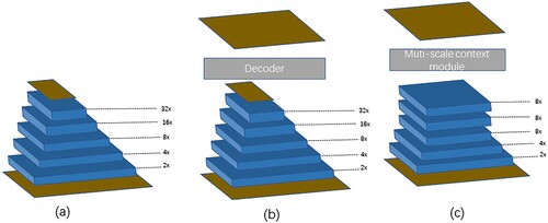
Dilated FCN is an ordinary FCN deformation, which adjusts the size of the receptive field and reduces the number of networks downsampling operations through atrous convolution, as shown in Figure 2(c). The Dilated FCN in the figure is 8x downsampling, and the semantics in the final feature map is richer and finer. The interpolation method can be used to restore the original resolution, but maintaining the resolution will result in a relatively large amount of computation.

Chen et al. (2018) proposed an encoder-decoder structure for semantic segmentation tasks, called deeplabv3+. Its encoder part is a deep convolutional network using atrous convolution, and conventional networks such as ResNet (He et al. 2016) and DS-pResNe (Dang, Pang, and Lee 2020) can be used. In this paper we used MLBSA as the main component of the encoder, which comes from the idea of Dilated FCN and employ atrous convolution to introduce information from a variety of receptive fields. Deeplabv3+ structure also includes a decoder module, which uses the traditional FCN idea to improve the final segmentation result, especially the boundary part of segmentation, by fusing low-level features with high-level features. From these perspectives, deeplabv3+ integrates the advantages of traditional FCN and Dilated FCN, overcomes their shortcomings, and improves its own performance.

The above models are mostly used for semantic segmentation tasks. The task of semantic segmentation is to classify each pixel in the image, whereas the task of hyperspectral image classification is to classify each pixel in the hyperspectral image. Although their tasks are similar in principle, the data of semantic segmentation is much richer than that of the hyperspectral image classification tasks. Therefore, the semantic segmentation model cannot be directly used for hyperspectral image classification. However, inspired by the semantic segmentation model, we can change the semantic segmentation model to make it competent for the task of hyperspectral image classification.

2.3 Attention mechanism

The attention mechanism was originally applied to machine translation, and has now become a research hotspot in various fields. Its core idea is to find the correlation between the original data and then highlight important features. Wang et al. (2018b) proposed type of non-local operations to capture long-range dependencies so as to find the connection between two pixels. Inspired by the idea of non-local mean filtering (Buades, Coll, and Morel 2005) in the field of image filtering, the author presented an operator that can be directly embedded in the non-local operation of the current network. The non-local operation can directly calculate the relationship between two positions to quickly capture long-range dependencies, which also cannot change the dimension of the feature map. Thus, this design can be easily inserted into the network. The main idea of traditional nonlocal filtering is to take a kernel as large as the original image as a weight to represent the similarity between other locations and the current computing location. In order to reduce parameters, nonlocal filtering adopts block level operation instead of point-to-point operation.

In the era of deep learning, non-local operations can be attributed to self-attention, and it can be expressed as Equation (1) (Wang et al. 2018b): (1) $y_i={\displaystyle \frac{1}{C\left(x\right)}\sum _{\mathrm{\forall }j}f\left(x_i,x_j\right)g\left(x_j\right)}$(1) where i is one of the positions of the output feature map, y is the final output of this position, j is the index of all positions, f is the correlation function that computes the i-th position and the j-th position (all other positions). g is the unary input function whose purpose is to change the information. C is a normalization function to ensure that the overall information remains unchanged before and after conversion. Although the module is relatively simple in the classification, it still leads to the problem of excessive calculation due to the size of the image.

Hu, Shen, and Sun (2018) designed a channel attention mechanism, The main operation is to weigh the corresponding weights of each channel of the original output channel through squeezing and excitation operations (each element of the corresponding channel is multiplied by the weights respectively) to obtain new weighted features. Squeeze operation is given in Equation (2) (Hu, Shen, and Sun 2018) and Excitation is given in Equation (3) (Hu, Shen, and Sun 2018): (2) $z_c=F_{sq}\left(u_c\right)={\displaystyle \frac{1}{H\times W}\sum _{i=1}^H\sum _{i=1}^W{u}_c\left(i,j\right),z\in R^c}$(2) (3) $s=F_{ex}\left(z,W\right)=\sigma \left(g\left(z,W_1\right)\right)=\sigma \left(W_{2}ReLU\left(W_{1}z\right)\right)$(3) In Equation (2), $z_c$ represents the value that encodes all pixel values in the c-th band, H and W represent the height and width respectively. $u_c\left(i,j\right)$ represents the pixel in the i-th row and the j-th column in the c-th band. While in equation(3),

$W_1\in R^{{\displaystyle \frac{C}{r}\times C}}$, $W_2\in R^{C\times {\displaystyle \frac{C}{r}}}$, $\sigma$ is the sigmoid activation function, the first fully connected layer plays the role of dimensionality reduction, r is the dimensionality reduction coefficient, and the last fully connected layer restores the original dimension and finally multiplies the learned activation value of each channel with the original output value, as shown in formulate (4) (Hu, Shen, and Sun 2018): (4) ${\tilde{x}}_c=F_{scale}\left(u_c,s_c\right)=s_c\cdot u_c$(4) Where ${\tilde{x}}_c$ represents the final output on the c-th band. The feature map finally obtained by the above operations learns the weight coefficients of each channel, so that the model has more ability to discriminate the features of each channel. Thus SEBlock is able to enhance useful bands and suppress useless bands, which has been shown to have the potential in improving the performance of CNNs.

3. EGL: effective global learning framework for hyperspectral image classification

The patch-based method generates redundant computation of overlapping regions which greatly increases the computational cost. To address this issue, we proposed an effective global learning (EGL) framework that can improve model speed and classification performance. In the EGL framework, instead of the patch-based method, we used the global learning method which can remove redundant computations and make full use of global spatial information to improve classification accuracy. The overall architecture of EGL is shown in Figure 3.

Figure 3. The architecture of EGL.

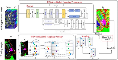
The purpose of the EGL framework is to learn mapping so that the input dimension is the same as the output dimension. The EGL framework consists of UGSS sampling strategy and BrsNet classification model. The UGSS sampling strategy first extracts training samples according to the type of ground objects, and then divides the training samples into hierarchical sequences of training samples according to the proportion. UGSS is able to divide most training samples, make the model converge smoothly and achieve good results. The feature learning part of BrsNet adopts improved linear bottleneck structure and spectral attention structure. The MLBSA structure integrates an improved linear bottleneck (MLB) and a spectral attention (SA) module. Through the linear bottleneck expansion operation and spectral attention channel selection, more distinguishing features can be learned to improve the classification performance.

3.1 Global learning

The core idea of global learning is that the input data of the model is a complete hyperspectral image. Compared with the patch-based method, global learning can reduce the redundancy and overcome the shortcoming of patch-based method unable to fully utilize the spatial information. For a hyperspectral image $X\in R^{C\times H\times W}$, the process of obtaining a $Y\in R^{class\times H\times W}$ that is the whole of the model can be represented by the mapping in Equation (5). (5) $f:R^{C\times H\times W}=R^{class\times H\times W}$(5) Among them, f represents a mapping to be learned by the global learning model, C is the number of bands of the input image, and class is the number of ground objects in the input image. H and W represent the height and width respectively.

The main difference between global learning and patch-based learning is that in global learning, all pixels are put into the network to participate in the feedforward operation, but only the pixels to be sampled can be learned and optimized. The traditional patch-based approach needs to first divide the data cube as the input of the model. In contrast, global learning does not require division operations, and it can directly input the data into the network. Therefore, the test time of model will be greatly shortened since division operation is no longer needed. In addition, all the spatial context information can be fully utilized, thereby improving the classification accuracy.

3.2 Universal Global Stochastic Stratified Sampling strategy

Although UGSS sampling is based on the sampling strategy proposed by GS2 in FPGA, it is suitable for more situations. When the size of training set increases, the number of samples of some classes may not be sufficient to provide enough samples in the dataset with fewer data. In view of the situation, UGSS sets a flexible proportion to ensure the normal progress of training. In the meantime, it speeds up the convergence speed of the model and makes the model have better generalization ability. The training samples use the entire image instead of a local area, and then the labeled pixel levels are assigned to a hierarchical sequence. Each species in every list is assigned by its own number and the number of mini-batches (donated as $\alpha$), which can avoid the situation that cannot be fully considered due to the small number of samples. Meanwhile, it also keeps a balance distribution between the various categories to a certain extent. For model training, the smaller the value of $\alpha$, the more stochastic gradients are obtained.

Table

Algorithm 1: Universal Global Stochastic Stratified Sampling

Input: G = {$g_i{\}}_{i=0}^N$:a set of labels of training N: number of class C: Number of samples taken for each class P: Percentage obtained when the amount of data is insufficient $\alpha$: Number of batch Output: T: Index list of training sample labels R$\leftarrow$[] //an empty list for k = 1 to N+1 do $I_k\leftarrow \left\{j\right|g_j=k,g_j\in G\}$ $I_k\leftarrow shuffle\left(I_k\right)$ if len($I_k$)≥C then $t\leftarrow I_k.pop\left(C\right)$//fetch C samples form $I_k$ R[k] = push(t)  else $t\leftarrow I_k.pop\left(len\left(I_k\right)\ast p\right)$ R[k] = push(t) end end $cnt\leftarrow 0$ $T\leftarrow \left[\right]$ // Store all batches While cnt <$\alpha$do for i = 0 to N do cd $\leftarrow$ceil(len(R[i])$/\alpha$ if len(R[j]) > 0 and len(R[j])<$\alpha$ then $cd\leftarrow 1$ end $\mathrm{l}\mathrm{e}\mathrm{f}\mathrm{t}\leftarrow cnt\ast cd$ // Starting point of one sampling if left ≥ len(R[i]) then continue end $right\leftarrow \left(cnt+1\right)\ast cd$ // End point of one sampling if cnt  = $\alpha -1$ then $right\leftarrow len\left(R\left[i\right]\right)$ $inds\leftarrow$ Take right-left elements in the i-th element in R end end T[cnt].push(inds) $cnt\leftarrow cnt+1$ end

Sampling algorithms is described in Algorithm 1. Specifically, we first classified all training samples according to the type of label, and then used the shuffle operation on the label set. Next, samples for each label were extracted separately. Finally, samples were obtained according to the number of samples for each label and the selected mini-batch. The training samples for each class were stratified by the quantity $\alpha$ to obtain a hierarchical sequence of pixels selected as training samples.

3.3 BrsNet in EGL

HSI has continuity, and the data of each band is relatively scattered. In order to accelerate the convergence speed and reduce the training time of the model, we need to normalize the zero mean of the whole HSI data, and then send it to the network. It is difference from the local learning framework, which normalize the zero mean of the data cube. The definition of standardized calculation is shown in Equation (6). (6) $X_{i,j}^n={\displaystyle \frac{X_{i,j}^n-{\overline{X}}^n}{{\sigma }^n}\left(1\le i\le W,1\le j\le H,1\le n\le N\right)}$(6) where $X_{i,j}^n$, represents the pixel value of the i-th row and j-th column of the n-th band of HSI, ${\overline{X}}^n$ indicates the average value of the pixels in the n-th band, and ${\sigma }^n$ is the standard deviation value of pixels in the n-th band; W, H and N represent the width, height and number of bands of the input HSI respectively.

BrsNet is an end-to-end classification model based on encoder-decoder structure. The encoder is responsible for the extraction of spectral spatial features, capturing the context information in the feature map through continuous convolution operations. Meantime, it combines all pixels of the input image and spectral attention to effectively learn the spectral-spatial information in HSI. The decoder restores the image to its original size and performs the final classification operation. Under the EGL framework, the input is all pixels, so the batch size is always equal to 1. In this case, using the Batch Normalization (BN) (Ioffe and Szegedy 2015) layer will lead to a rapid increase in the error, so the Group Normalization (GN) (Wu and He 2018) layer is used as an alternative to reduce errors. The detailed structure of BrsNet is shown in Figure 4.

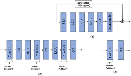
Figure 4. The structure diagram of BrsNet.

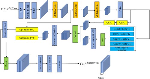
In the composition structure of BrsNet, it is mainly composed of an encoder network and a decoder network. There is an SSA module, 1×1 convolution, and a GN layer before the encoder network, which is used to adjust the number of spectra accordingly. After adjustment, the MLBSA unit is stacked. The output of MLBSA enters the dual-branch structure for final spectral spatial feature extraction, and the output of the dual-branch structure is upsampled by 8x to restore the spatial dimension of the tensor to the same as the original image. First, a shortcut connection are taken from the encoder network, and then 2x upsampling are used to restore the output of the shortcut connection to the same dimension as the output of the dual-branch structure. Finally, the output of the shortcut connection and the output of the double branch structure are combined by the concat operation, and the final output is obtained after adjusting the dimension through Con-GN-ReLU-Con-GN-ReLU-Con. The output dimension is$C\times H\times W$, where C is the number of species, H is the height, and W is the width. We give the detailed design of each module in the following content.

3.3.1 Structure of MLBSA

Assuming that the neural network is considered as a superposition of n $L_i$ layers, the output tensor of the input data passing through the superposition of these layers is $h_i\times w_i\times d_i$. We regard this series of convolution and activation layers as forming a n stream of interest, which is the data content that we are interested in. Generally speaking, we can map the data content of interest into a low-dimensional subspace for processing (for example, using $1\times 1$ convolution to reduce the spectral dimension dimension) in the neural network. Maintaining the integrity of the content of interest is of great significance to improve the classification performance.

According to the description of the work in (Sandler et al. 2018), using nonlinear activation functions (such as ReLU) will lose useful information in the activation layer. Compared with the bottleneck layer, the linear bottleneck layer uses $1\times 1$ convolution for expanding to map the low-dimensional feature space to the high-dimensional space rather than reducing dimensionality. Due to the addition of the expansion operation, the operation on the tensor is reversed compared to the traditional convolution of from high-dimensional to low-dimensional, so the residual block composed of the linear bottleneck structure is called the inverted residual. The use of inverted residuals can preserve the data content of interest to a large extent, and is suitable for the classification of ordinary images.

For our proposed MLBSA structure, when data from low-dimensional space is mapped to high-dimensional space, we still use a nonlinear activation function, because of HSI itself having the characteristic of high-dimensionality. When low-dimensional tensor is mapped to high-dimensional space, its own dimension is very high and the data content of interest is kept relatively intact. Therefore, we use the nonlinear activation function to avoid losing too much information.

Meanwhile, in the process of feature extraction, using high-dimensional tensors to extract features can obtain sufficient information to make extracted features more conducive to classification. Compared with the dimension of the feature map after the expansion operation, the dimension of the output feature map is low. Therefore, we did not use an activation function in the last layer, as it will cause a large loss of useful information.

Figure 5 shows the structure of our proposed MLBSA and its components. As shown in Figure 5(a), we add a downsampling module (shown in Figure 5(c)) after two MLB structures shown in Figure 5(b), which is used to extract abstract features and save computational resources. The input of the first MLB structure is added with the output of the downsampling module through skip connections. Since the convolution kernel used by the downsampling module is 3 and the stride is 2, the dimensions of the two parts do not match. Therefore, we used zero-padded skip connections (Han, Kim, and Kim 2017) combined with average pooling to ensure that the dimensions of the two parts were the same for the addition operation. The advantage of zero-padded is that there are no extra parameters while guaranteeing a normal addition operation.

Figure 5. Three structures: (a) The structure of an MLBSA, (b) The structure of an MLB, and (c) The structure of downsampling.

3.3.2 Shuffle spectral attention

The basic SEBlock simply assigns weights to each spectral channel through $3\times 3$ convolution and performs weighting operations on the original data, which can remove useless spectral data. It addresses in ECANet (Wang et al. 2019) that proper cross-channel interaction is important to learn high-performance and efficient channel attention. The purpose of the two FC layers of SEBlock is to capture nonlinear cross-channel interaction, but it will negatively impact the effect to some extent, due to its inherent degradation dimension. Most of the current methods focus on developing complex attention modules for better performance, but it will inevitably increase the parameters of the model. Thus, we improved on the basis of SEBlock and designed a shuffle spectral attention module without significantly adding more parameters.

The specific structure of the SSA module is shown in Figure 6. In SSA, we added a shuffle operation before global pooling to increase interactivity between channels. Then the spectral dimension was normalized using a GN layer. The shuffle operation can enable sufficient information interaction between channels. The combination of shuffle operation and MLB structure can continuously learn effective spectral features and spatial features thereby improving the effectiveness of the model. The details of the SSA module is described below. The SSA model starts with a squeezing operation identical to SEBlock, which is defined in Equation (7). (7) $z_c=F_{sq}\left(u_c\right)={\displaystyle \frac{1}{H\times W}\sum _{i=1}^H\sum _{i=1}^W{u}_c\left(i,j\right),z\in R^c}$(7) where $z_c$ represents the value that encodes all pixel values in the c-th band, H and W represent the height and width respectively. $u_c\left(i,j\right)$ represents the pixel in the i-th row and the j-th column in the c-th band.

Figure 6. The specific structure of the SSA module.

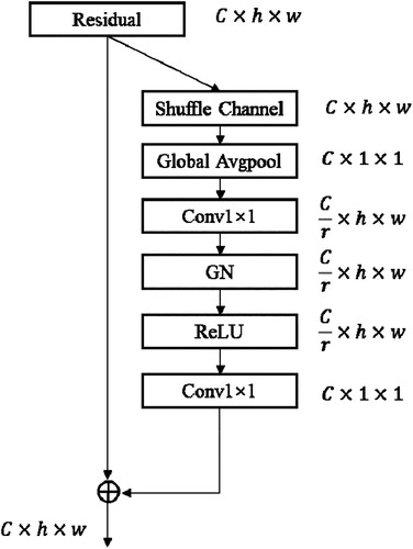
Next, the SSA module has the excitation part employing the shuffle operation of the band, which is different from SEBlock. The shuffle process is described in Equation (8): (8) $s=F_{ex}\left(z,W\right)=W_2\left(ReLU\left(\left(GN\left(W_1\left(Shuffle\left(z\right)\right)\right)\right)\right)\right)$(8) Where s represents the output of SSA module. $W_1\in R^{{\displaystyle \frac{C}{r}\times C}}$, $W_2\in R^{C\times {\displaystyle \frac{C}{r}}}$, they use the shuffle operation to disrupt the original fixed order between channels and increase the interactivity between channels. Then the first fully connected layer plays the role of dimensionality reduction, where r is the dimensionality reduction coefficient, the last fully connected layer restores the original dimension.

Finally, the learned activation value of each channel is added to the original output value to obtain the final feature map from Equation (9), ${\tilde{x}}_c$represents the final output on the c-th band. (9) ${\tilde{x}}_c=F_{scale}\left(u_c,s_c\right)=s_c+u_c$(9) The final output feature map is regarded as the result of measuring the importance of each feature channel in the model, and the recalibration of the original features in the channel dimension is completed.

3.3.3 Feature extraction of two-branch structure

In BrsNet, we designed a dual-branch structure in order to fully extract spectral and spatial features. The dual-branch structure consists of Atrous Spatial Pyramid Pooling (ASPP) and non-local modules.

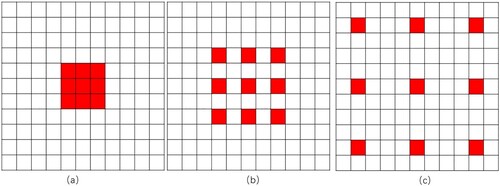
The atrous convolution is the key to the atrous spatial pyramid pooling (ASPP) (Chen et al. 2017). It can control the size of the receptive field without changing the size of the feature map, which is conducive to the extraction of spatial information at multiple scales. By changing the dilation rate, the change of the receptive field can be controlled. The size of the corresponding receptive field is shown in Figure 7. In the ASPP branch, we use five branches consisting of one global average pooling (GAP) and four atrous convolutional layers with dilation rate of 1, 12, 24, and 36 respectively. We need to use upsampling on the GAP to make sure that the GAP output and the atrous convolution output have the same dimension. After executing a concat operation on their results, a $1\times 1$convolution is adopted to adjust the spectral dimension of the output tensor of the concat operation to be consistent with the spectral dimension of the ASPP input tensor. The processed output incorporates information extracted by convolutions of various receptive field sizes.

Figure 7. Receptive field size of atrous convolution under different dilation rate: (a) Receptive field of atrous convolution with dilation rate of 1, (b) Receptive field of atrous convolution with dilation rate of 2, and (c) Receptive field of atrous convolution with dilation rate of 4.

For traditional non-local modules, the computation time is very large, because all pixels are considered in the computation. The CCA can aggregate the pixels in the horizontal and vertical directions and reduce the size of attention map. In CCA, the dimension of the input is equal to the dimension of the output, so the module can be embedded anywhere in the neural network for non-local information extraction. We use the method of stacking the CCA twice avoid the sparse problem. It means that the output of the module of the first CCA will be input into the CCA module again to get the final output. In the first CCA module, the lower left corner block only has the information of the upper left corner block and the lower right corner block. By stacking the second CCA module, the upper left corner block and the lower right corner block already contain the information of the upper right corner block. The information of the upper right corner block can flow into the lower left corner block, because the stacking of the two CCA modules is equivalent to traversing all blocks.

Atrous spatial pyramid pooling includes multiple atrous convolutions with different sampling rates, so that the receptive field of each atrous convolution is different which can include multi-scale spatial information. The non-local module is used to weigh the pixels from a global perspective. Due to the existence of the UGSS sampling strategy, the input is all the pixels of the HSI at each time. Therefore, the combination of the non-local module and ASPP can extract spatial information from the global and local multi-scales respectively. The dual-branch structure obtains rich global and local spatial information, and fully exploits the potential of spatial information in HSI while adding as few parameters as possible. The combination of the dual-branch structure and SSA module improves the performance of the classification model from the spatial and spectral perspectives, respectively.

4. Experimental results and analysis

To completely analyse the classification performance of our proposed model, we will compare it with several typical HSI classification methods that have emerged in recent years, including SVM-RBF (Melgani and Bruzzone 2004), 1D-CNN (Hu et al. 2015), M3D-DCNN (He, Li, and Chen 2017), SSRN (Zhong et al. 2017), DBDA (Li et al. 2020), A²S²K-ResNet (Roy et al. 2021) and SNN-SSEM (Liu et al. 2022). These methods are extensively experimented on three datasets: 16-category Indian Pines dataset, 9-category Pavia University dataset and 16-category Salinas dataset. The model designed in this paper was implemented by Python version 3.7.10 and the deep learning framework of PyTorch version 1.8.0. The computer hardware was Intel (R) Xeon (R) E5-2682 [email protected] GHz CPU, the memory size was 32 GB, and the NVIDIA GeForce RTX 3060GPU.

4.1 Experimental settings

• Model parameters: The reduction ratio r in the spectral attention module is set to 16, group-normalized number of groups is set to 16, and the expansion of the MLB is set to 2.

• Optimization: For all experiments, the EGL framework was optimized using SGD (Robbins and Monro 1951) with the addition of a ‘poly’ learning rate policy, the momentum is set to 0.9, and no data expansion strategy is adopted. The initial learning rate of the optimizer is 0.001, and the learning rate after each iteration is the current learning rate multiplied by ${\left(1-\frac{iter}{max\mathrm{\_}iter}\right)}^{0.9}$. iter is the current number of iterations, and max_iter is the total number of iterations. max_iter is set to 1000 here. If there is no description, the $\alpha$ of the UGSS sampler is set to 10, and the P is set to 0.8.

• Metrics: To evaluate the performance of the proposed method, three commonly used metrics are adopted: Overall Accuracy (OA), Average Accuracy (AA), and Kappa Coefficient (Kappa).

4.2 Experiment 1: Indian Pine Dataset

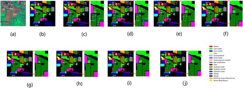
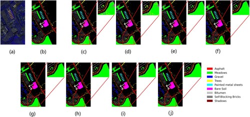
Indian Pines dataset (IP) imaged by AVIRIS, cropped at 145$\times$145 size for annotation. 200 bands were selected as research objects. The dataset has 10249 ground object pixels and the rest are background pixels. Figure 8 shows the classification results of the different models in IP dataset, as well as the false color images of original HSI and its corresponding ground-truth maps. Figure 8(a,b) represent a false-color composite of the image with the corresponding ground truth.

Figure 8. Visualization of the classification maps for the IP dataset: (a) false color image, (b) ground-truth map, (c) RBF-SVM, (d) 1D-CNN, (e) M3D-DCNN, (f) SSRN, (g) DBDA, (h) A²S²K-ResNet, (i) SNN-SSEM, and (j) EGL.

We randomly selected 200 samples of each type of object as the training set. However, in the Indian pine data set, the number of individual samples was less than 200. At this time, a proportion P was selected to take the total number as the training set. The value of P here is set to 0.8 unless otherwise specified. After that, 75% of the training samples were taken as the training set, and the rest was used as the validation set. The training sample adopted the UGSS sampling strategy. Table 1 lists the number of training samples of each type. The selection of training samples was randomly selected from random number seed.

Table 1. The details of the IP dataset ground objects samples and the division of the training set and test set.

Class	Class name	Total	Train	Test
C1	Alfalfa	46	37	9
C2	Corn-notill	1428	200	1228
C3	Corn-mintill	830	200	630
C4	Corn	237	200	37
C5	Grass-pasture	483	200	283
C6	Grass-trees	730	200	530
C7	Grass-pasture-mowed	28	23	5
C8	Hay-windrowed	478	200	278
C9	Oats	20	16	4
C10	Soybean-notill	972	200	772
C11	Soybean-mintill	2455	200	2255
C12	Soybean-clean	593	200	393
C13	Wheat	205	200	5
C14	Woods	1265	200	1065
C15	Buildings-Grass-Trees-Drives	386	200	186
C16	Stone-Steel-Towers	93	75	18
	Total	10249	2551	7698

Figure 8(c–j) show the classification graphs of all the compared methods. Seen from Figure 8, the CNN-based classification methods tend to perform better than the SVM-RBF in classification result. In the renderings, the CNN-based method performs more smoothly than SVM-RBF, because CNN can extract deep features and consider neighborhood pixels. By comparing the ground-truth map of the IP dataset, overall, our proposed method has more regions corresponding to the ground-truth map than other methods. At the same time, in the area we circled by the red rectangle, it can be seen that for the ‘Corn-notill’ and the ‘Soybean-mintill’, our proposed method has fewer misclassifications, suggesting that our method has better performance and classification accuracy.

To further measure the performance of BrsNet, we conducted 10 experiments for each selected model. The three evaluation indicators including OA, AA and Kappa coefficient were calculated as mean ± standard. Table 2 gives the results obtained by 10 experiments. The number of the item with the highest classification accuracy in each category is bolded. It can be seen that our method outperforms all the compared models based on three evaluation indicators. Among of these methods, our EGL method achieves an accuracy of more than 99% for both similar-band features and small-sample data. Among these methods, our proposed method achieves more than 99% accuracy for most of the similar band features and small sample data. Although the accuracies of SSRN, DBDA, A²S²K-ResNet and SNN-SSEM are also excellent, they still lag behind our method. These results reveal that our model can select the bands more accurately by the SSA module and improve the classification accuracy of small sample data by the UGSS strategy. In additional, our method has the smallest standard deviation, suggesting a better stability of our proposed method compared to others.

Table 2. Classification results on the IP dataset with 200 labeled samples.

Class	SVM-RBF	1D-CNN	M3D-DCNN	SSRN	DBDA	A^2S^2K-ResNet	SNN-SSEM	Proposed
C1	58.77	92.22	96.67	100	88.1	100	100	100
C2	77.96	81.68	86.9	98.11	98.62	98.63	98.3	99.26
C3	71.68	81.44	90.59	98.02	98.34	99.11	99.57	97.79
C4	19.93	92.97	99.73	91.62	94.22	100	100	100
C5	89.84	94.59	98.34	99.08	99.09	99.54	99.79	100
C6	97.01	97.81	99.74	99.61	98.29	99.92	99.89	100
C7	75.88	98	100	96.67	83.83	100	100	100
C8	99.13	98.67	99.93	99.93	99.96	100	100	100
C9	51.78	100	100	100	93.33	100	100	100
C10	72.46	90.4	91.27	92.71	94.45	98.65	99.24	99.75
C11	90.22	72.36	78.29	99.33	99.45	97.84	97.66	99.34
C12	73.16	91.6	95.24	98.07	98.91	99.11	99.31	99.47
C13	72.62	100	100	96.67	93.81	100	100	100
C14	97.9	91.35	95.76	99.78	99.79	99.53	99.62	100
C15	57.92	85.16	98.44	97.03	98.59	99.89	100	100
C16	78.59	98.33	100	90.62	85.08	100	99.44	100
OA	82.32 ± 0.753	84.07 ± 1.05	88.95 ± 1.46	98.16 ± 0.46	98.48 ± 0.521	98.81 ± 0.28	98.83 ± 0.22	99.46 ± 0.09
AA	74.05 ± 1.71	91.66 ± 0.95	95.68 ± 0.64	97.33 ± 0.955	95.24 ± 2.277	99.51 ± 0.11	99.55 ± 0.12	99.73 ± 0.03
Kappa	79.38 ± 0.872	81.44 ± 1.14	87.07 ± 1.66	97.83 ± 0.543	98.20 ± 0.615	98.59 ± 0.33	98.61 ± 0.26	99.35 ± 0.1

4.3 Experiment 2: Pavia University Dataset

The Pavia dataset (PU) is part of the hyperspectral data imaged by ROSIS-03. Typically, an image consisting of 103 spectral bands is used. The data size is 610$\times$340, there are only 42776 feature pixels in total, and the rest are background pixels. Figure 9 shows the classification results of the different models in PU dataset, as well as the false color images of original HSI and its corresponding ground-truth maps. Figure 9(a,b) represents a false-color composite of the image with the corresponding ground truth.

Figure 9. Visualization of the classification maps for the PU dataset: (a) false color image, (b) ground-truth map, (c) RBF-SVM, (d) 1D-CNN, (e) M3D-DCNN, (f) SSRN, (g) DBDA, (h) A²S²K-ResNet, (i) SNN-SSEM, and (j) EGL.

Table 3 shows the number of training samples for each type, and the selection of training samples is randomly selected from random number seed.

Table 3. The details of the ground object sample in the PU dataset and the division of the training set and test set.

Class	Class Name	Total	Train	Test
C1	Asphalt	6631	200	6431
C2	Meadows	18649	200	18449
C3	Gravel	2099	200	1899
C4	Trees	3064	200	2864
C5	Painted metal sheets	1345	200	1145
C6	Bare Soil	5029	200	4829
C7	Bitumen	1330	200	1130
C8	Self-Blocking Bricks	3682	200	3482
C9	Shadows	947	200	747
	Total	42776	1800	40976

Figure 9(c–j) shows the classification graphs of all the methods. From the results of Figure 9, the CNN-based classification method has better performance than SVM-RBF in the Pavia dataset. The 1D-CNN method has serious salt and pepper noise like SVM-RBF because it does not use spatial-spectral information, which make it difficult to distinguish the type of buildings with different roof materials using only spatial information. For SSRN, DBDA, A2S 2K-ResNet and SNN-SSEM methods,overall they have a good performance, but they have poor classification accuracy on some ground objects. This can also be seen from the red rectangular area in the classification map of each method, and the above methods still have small misclassifications in the rectangular area. However, our proposed method has better classification results. The number of samples in the PU dataset is relatively sufficient. However, there are indistinguishable ground coverings, such as gravel, Bare Soil and Bricks, which will have negative effect on the classification. Whereas for our EGL methods, we used the SSA module to extract spectral information and global learning and the dual branches of ASPP and CCA, which will accurately separate all samples.

Table 4 shows the average precision of each type of ground objects in ten experiments of the six methods, and the mean$\pm$standard deviation of the OA, AA, and Kappa coefficients. The overall accuracy is mostly above 90%. However, as mentioned above, for the indistinguishable ground cover of the PU dataset, such as Gravel, Bare Soil and Bricks, the classification effect is generally poor in other methods. In contrast, in our proposed method, the accuracy of Graveland Bare soil reaches 100%, and the accuracy of bricks reaches 99.96%. Seen from Figure 9, we can also clearly find that for the other models, some of these types of ground cover are misclassified. In contrast, the accuracy of our method has reached saturation (over 99.9%). This shows that our method also has great classification performance for indistinguishable objects.

Table 4. Classification Results on the PU Dataset with 200 Labeled Samples.

Class	SVM-RBF	1D-CNN	M3D-DCNN	SSRN	DBDA	A^2S^2K-ResNet	SNN-SSEM	Proposed
C1	96.83	85.27	94.59	99.9	99.56	98.82	99.69	99.98
C2	97.41	88.08	96.67	99.11	99.92	99.25	99.59	99.97
C3	76.04	82.91	93.52	92.14	98.98	99.08	98.92	100
C4	87.68	96.49	98.38	99.47	97.27	99.41	99.32	99.63
C5	97.56	99.74	100	100	99.9	99.99	100	100
C6	76.75	91.5	97.73	94.2	96.27	99.66	99.93	100
C7	66.36	91.6	97.69	98.17	99.32	99.95	100	100
C8	85.76	85.15	94.18	97.4	97.1	99.26	99.45	99.96
C9	99.87	99.88	99.83	99.78	97.55	100	99.8	100
OA	90.34 ± 0.678	88.78 ± 2.25	96.41 ± 0.84	97.9 ± 1.835	98.90 ± 0.607	99.29 ± 0.31	99.61 ± 0.21	99.95 ± 0.005
AA	87.14 ± 0.694	91.18 ± 0.86	96.95 ± 0.43	97.80 ± 1.31	98.46 ± 0.630	99.49 ± 0.17	99.63 ± 0.18	99.95 ± 0.005
Kappa	87.22 ± 0.868	85.26 ± 2.78	95.2 ± 1.11	97.20 ± 2.44	98.53 ± 0.809	99.05 ± 0.41	99.48 ± 0.29	99.94 ± 0.006

4.4 Experiment 3: Salinas Dataset

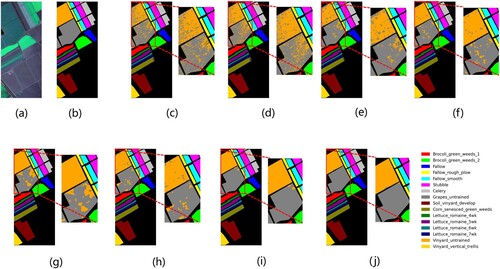
The Salinas Dataset (SA) was captured by AVIRIS and selected images in 204 bands. The size of the image is 512$\times$217, of which 54129 are ground object pixels and the rest are Beijing pixels. These pixels are grouped into 16 categories including Stubble, Celery and so on. Figure 10 shows the classification results of the different models in SA dataset, as well as the false color images of original HSI and its corresponding ground-truth maps. Figure 10(a,b) represents a false-color composite of the image with the corresponding ground truth.

Figure 10. Visualization of the classification maps for the SA dataset: (a) false color image,, (b) ground-truth map, (c) RBF-SVM, (d) 1D-CNN, (e) M3D-DCNN, (f) SSRN, (g) DBDA, (h) A²S²K-ResNet, (i) SNN-SSEM, and (j) EGL.

Table 5 lists the number of training samples for each type, and the selection of training samples is randomly selected from random number seed.

Table 5. The details of the ground object sample in the SA dataset and the division of the training set and test set.

Class	Class name	Total	Train	Test
C1	Brocoli_green_weeds_1	2009	200	1809
C2	Brocoli_green_weeds_2	3726	200	3526
C3	Fallow	1976	200	1776
C4	Fallow_rough_plow	1394	200	1194
C5	Fallow_smooth	2678	200	2478
C6	Stubble	3959	200	3759
C7	Celery	3579	200	3379
C8	Grapes_untrained	11271	200	11071
C9	Soil_vinyard_develop	6203	200	6003
C10	Corn_senesced_green_weeds	3278	200	3078
C11	Lettuce_romaine_4wk	1068	200	868
C12	Lettuce_romaine_5wk	1927	200	1727
C13	Lettuce_romaine_6wk	916	200	716
C14	Lettuce_romaine_7wk	1070	200	870
C15	Vinyard_untrained	7268	200	7068
C16	Vinyard_vertical_trellis	1807	200	1607
	Total	54129	1800	50929

The classification results of all the methods are shown in Figure 10(c–h). The accuracy of our method is the best in most of the 16 categories. For the class types C8 and C15, most of methods have lower classification accuracy due to their similarity, but our method can get the good accuracy on them. The results illustrate the effectiveness of the EGL framework.

Table 6 shows the average precision of each type of ground object and the mean ± standard deviation of the OA, AA, and Kappa coefficients. Since the number of samples in the SA dataset is sufficient, all methods achieve 90% accuracy. However, the performance of C8 and C15 of all models is not satisfactory. Although DBDA's C8 has an accuracy of more than 98%, C15 only has 91.81% accuracy, The accuracy of C15 is better on SNN-SSEM, but the accuracy of C8 still fails to reach 99%. Our method achieves the accuracy of 99.71% and 98.78% in C8 and C15, respectively. The reason is that our method used multiple techniques that can fully exploit the role of spatial features in HSI classification, such as the SSA UGSS sampling strategy and dual branches of CCA and ASPP. The results also show that the EGL framework is effective and can be generalized in other situations.

Table 6. Classification Results on the SA Dataset with 200 Labeled Samples.

Class	SVM-RBF	1D-CNN	M3D-DCNN	SSRN	DBDA	A^2S^2K-ResNet	SNN-SSEM	Proposed
C1	99.87	99.21	99.98	100	99.91	100	100	100
C2	99.73	99.7	99.92	99.98	100	100	100	100
C3	97.06	99.48	99.94	99.99	99.81	100	100	100
C4	98.56	99.61	99.7	99.39	99.42	99.98	99.92	99.64
C5	99.21	98.58	99.1	99.79	99.63	99.48	99.53	99.10
C6	99.97	99.81	99.99	99.99	100	100	100	100
C7	99.37	99.7	99.84	99.98	99.99	100	100	100
C8	82.45	80	86.24	93.93	98.66	93.01	98.95	99.71
C9	99.37	99.68	99.91	99.96	99.85	100	100	100
C10	91.74	93.66	96.73	98.44	98.49	99.27	99.89	99.20
C11	96.22	98.42	99.62	99.46	98.41	99.97	100	99.50
C12	98.69	99.83	100	99.96	100	100	99.99	100
C13	99.05	99.37	99.93	99.97	99.96	100	100	100
C14	93.99	97.92	99.6	99.78	99.37	99.83	99.98	100
C15	70.95	71.59	85.97	92.17	91.81	95.83	99.43	98.78
C16	97.28	98.67	99.14	99.79	100	99.88	99.99	100
OA	91.02 ± 0.662	90.99 ± 0.58	94.74 ± 0.59	97.36 ± 0.657	98.23 ± 0.629	97.82 ± 0.45	99.66 ± 0.19	99.66 ± 0.06
AA	95.22 ± 0.256	95.95 ± 0.23	97.85 ± 0.18	98.91 ± 0.196	99.08 ± 1.293	99.2 ± 0.16	99.85 ± 0.07	99.75 ± 0.03
Kappa	89.96 ± 0.74	89.92 ± 0.64	94.12 ± 0.65	97.04 ± 0.74	98.02 ± 1.440	97.56 ± 0.5	99.62 ± 0.21	99.62 ± 0.07

4.5 Experiment 4: module discussion

In order to verify the effectiveness of the MLB, dual-branch structure, and the SSA module, we carried out five experiments using our proposed framework EGL. All the experiments were conducted on the Indian Pine dataset with a relatively small number of samples. The baseline method only used the UGSS sampling and BrsNet without using any modules designed in this paper. The experimental results are shown in Table 7. The mean OA of baseline method has achieved 99.08%. After adding SEBlock, the accuracy rate was slightly improved to 99.09%. When adding continuously the MLB structure, the average value of OA has reached 99.29%. Next, we introduced the double-branch structure on the abovementioned method where the accuracy rate has increased to 99.33%. Finally, we adopted the SSA module instead of SEBlock to test the effective of SSA, and the average accuracy rises to 99.46%. The results reveal that the MLB, dual-branch structure and SSA designed in our EGL framework helped improve the performance of classification.

Table 7. The experimental results of the module effectiveness experiment under the IP data set.

Method	SEBlock	SSA	Double branch	MLB (modified linear Bottleneck)	OA	AA	Kappa
BrsNet(Base)	×	×	×	×	99.08 ± 0.07	99.69 ± 0.03	98.90 ± 0.07
BrsNet(SEBlock)	√	×	×	×	99.09 ± 0.07	99.67 ± 0.02	98.92 ± 0.08
BrsNet(SEBlock + MLB)	√	×	×	√	99.29 ± 0.09	99.67 ± 0.04	99.16 ± 0.11
BrsNet(SEBlock + MLB + Double branch)	√	×	√	√	99.33 ± 0.08	99.68 ± 0.04	99.21 ± 0.1
BrsNet(MLBSA + Double branch)	×	√	√	√	99.46 ± 0.09	99.73 ± 0.03	99.35 ± 0.1

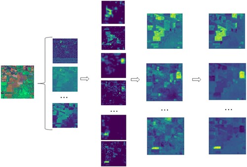
Meanwhile, we visualized the feature map of our proposed method under the IP dataset to further illustrate the effectiveness of our proposed method. The visualization of the feature maps in the classification process is shown in Figure 11. The first group is the initial feature maps. The highlighted areas and clear textures of the feature maps in the second group suggested that our method has extracted space and spectrum. The performance is well in terms of features. After combining space and spectrum features, the third group of feature map visualizations show that the classification was close to the final classification result, which is shown in the last group. The number of channels of the feature map output by our method is equal to the type of ground objects. Each channel of the output feature map corresponds to the classification result of a ground object, and the accurate highlighted area of the classification result fully demonstrates the effectiveness of our proposed method in the hyperspectral image classification task.

Figure 11. Results of feature map visualization under IP dataset.

4.6 Experiment 5: speed discussion

We compare the training and testing times of all methods on the three datasets. As shown in Table 8, compared with SSRN, DBDA, A2S 2K-ResNet and SNN-SSEM, which have great classification performance, our method had better classification performance on IP dataset and had a shorter training time. The training time of our proposed method is slightly longer than that of DBDA on the PU and SA datasets. When DBDA reaches the specified metric during training, it will stop training. Thus it has shorter training time on both PU and SA datasets, but its classification accuracy is lower than our proposed method. In addition, our method is a global learning method, and the test data of the global learning method is a complete image instead of a patch for each test pixel. Therefore, reducing the redundancy of overlapping regions between adjacent pixel patches calculation will greatly reduce the test time of the model. The test time of our proposed method is only 0.06s, 0.33s and 0.21s on IP, PU and SA datasets, respectively. In a word, the proposed framework is promising for future application.

Table 8. Training and testing time of different models on three HSI datasets.

		IP	PU	SA
SVM-RBF	Train.(s) Test.(s)	749.2 5.63	132.6 11.235	408 19.43
1D-CNN	Train.(s) Test.(s)	60.31 0.46	42.04 2.38	76.97 3.05
M3D-DCNN	Train.(s) Test.(s)	139.75 0.94	75.23 3.61	181.5 6.46
SSRN	Train.(s) Test.(s)	3338.215 3.87	2230.5 18.85	4124.1 25.13
DBDA	Train.(s) Test.(s)	448.9 9.56	196.01 31.78	598.7 66.1
A^2S^2K-ResNet	Train.(s) Test.(s)	3118.18 2.9	5050.26 17.55	6421.37 27.94
SNN-SSEM	Train.(s) Test.(s)	5491.51 491.63	4293.88 324.46	8289.87 57.38
EGL	Train.(s) Test.(s)	223.7 0.06	1134.2 0.33	686.1 0.21

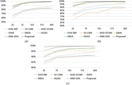
4.7 Experiment 6: the impact of the number of training samples

To investigate the effect of the number of training samples on EGL, we conducted extensive experiments on IP, PU and SA datasets. The results are shown in Figure 12. Overall, our method achieved better results than other methods at various sample sizes. The reduction in the number of samples will degrade the performance of EGL. For the PU dataset and SA dataset, when the average number of training samples per class was 25, the decrease in OA was relatively small. This suggests that the method we used is stable. On the IP dataset, our method degraded the accuracy more rapidly when the sample size was small compared to the PU and SA datasets, indicating that the classification of the PU and SA datasets using EGL is more stable than using the IP datasets. We speculate that this is because of the higher spatial resolution of these two datasets, and our method used global learning and a dual-branch structure to allow the spatial information to contribute significantly to the performance. In the PU datasets with the largest spatial resolution, the contribution of spatial information to performance has reached saturation. Compared with the PU dataset, the classification accuracy of the SA dataset has a smaller decrease in the 25 samples. We speculate that it is because the SA dataset has more bands, and the effectiveness of the SSA module for extracting spectral information lead to less degradation in classification accuracy.

Figure 12. Overall Accuracy versus the number of training samples per class: (a) Experimental results under IP dataset, (b) Experimental results under PU dataset, and (c) Experimental results under SA dataset.

5. Conclusions

In this paper, we proposed a general global learning framework, the EGL framework, which can improve the speed and accuracy of HSI classification. Under the EGL framework, we adopted a UGSS sampling strategy to ensure the convergence of the model. We also used the BrsNet network in our framework based on encoder-decoder structure with the whole hyperspectral image without any processing as the input. We designed the MLBSA structure by MLB structure and SSA module that can fully extract spectral spatial features. In additional, we adopted the dual-branch structure and SSA module to excavate the spatial and spectral information in HSI. We conducted several experiments on three well-known datasets. The results indicate that our method have the higher performance in hyperspectral image classification. Comparing the performance of our proposed method with other models, our method has a significant advantage in test time. Meanwhile, the proposed framework EGL not only is effective, but also has a good generalization ability.

In the future, we will do some works to improve the effectiveness of the EGL framework. It can be done by stopping the training of the EGL classification model when a specified metrics is reached, which could potentially improve the training time. Furthermore, our EGL framework can also be extended to other hyperspectral image classification scenarios to improve its generalization ability.

Disclosure statement

No potential conflict of interest was reported by the author(s).

Additional information

Funding

This research was funded by National Natural Special Foundation of Central Government to Guide Local Science & Technology Development (2021Szvup032).

References

- Abbate, Giulia, L. Fiumi, C. De Lorenzo, and Ruxandra Vintila. 2003. “Evaluation of Remote Sensing Data for Urban Planning. Applicative Examples by Means of Multispectral and Hyperspectral Data.” In 2003 2nd GRSS/ISPRS Joint Workshop on Remote Sensing and Data Fusion over Urban Areas, 201–205. IEEE.
- Buades, Antoni, Bartomeu Coll, and J.-M. Morel. 2005. “A non-local algorithm for image denoising.” In 2005 IEEE Computer Society Conference on Computer Vision and Pattern Recognition (CVPR’05), Vol. 2, 60–65. IEEE.
- Chen, Liang-Chieh, George Papandreou, Iasonas Kokkinos, Kevin Murphy, and Alan L Yuille. 2017. “Deeplab: Semantic Image Segmentation with Deep Convolutional Nets, Atrous Convolution, and Fully Connected Crfs.” IEEE Transactions on Pattern Analysis and Machine Intelligence 40 (4): 834–848.
- Chen, Liang-Chieh, Yukun Zhu, George Papandreou, Florian Schroff, and Hartwig Adam. 2018. “Encoder-Decoder With Atrous Separable Convolution for Semantic Image Segmentation.” In Proceedings of the European Conference on Computer Vision (ECCV), 801–818.
- Coops, N. C., M.- Smith, M. E. Martin, and S. V. Ollinger. 2003. “Prediction of Eucalypt Foliage Nitrogen Content from Satellite-Derived Hyperspectral Data.” in IEEE Transactions on Geoscience and Remote Sensing 41 (6): 1338–1346. doi:10.1109/TGRS.2003.813135.
- Dang, Lanxue, Peidong Pang, and Jay Lee. 2020. “Depth-wise Separable Convolution Neural Network with Residual Connection for Hyperspectral Image Classification.” Remote Sensing 12 (20): 3408.
- Deepa, P., and K. Thilagavathi. 2015. “Feature extraction of hyperspectral image using principal component analysis and folded-principal component analysis.” In 2015 2nd International Conference on Electronics and Communication Systems (ICECS), 656–660. IEEE.
- Du, Qian. 2007. “Modified Fisher’s Linear Discriminant Analysis for Hyperspectral Imagery.” IEEE Geoscience and Remote Sensing Letters 4 (4): 503–507.
- Fang, Leyuan, Shutao Li, Xudong Kang, and Jon Atli Benediktsson. 2014. “Spectral-spatial Hyperspectral Image Classification via Multiscale Adaptive Sparse Representation.” IEEE Transactions on Geoscience and Remote Sensing 52 (12): 7738–7749.
- Fu, Anyan, Xiaorui Ma, and Hongyu Wang. 2018. “Classification of Hyperspectral Image Based on Hybrid Neural Networks.” In IGARSS 2018-2018 IEEE International Geoscience and Remote Sensing Symposium, 2643–2646. IEEE.
- Han, Dongyoon, Jiwhan Kim, and Junmo Kim. 2017. “Deep Pyramidal Residual Networks.” In Proceedings of the IEEE Conference on Computer Vision and Pattern Recognition, 5927–5935.
- He, Mingyi, Bo Li, and Huahui Chen. 2017. “Multi-scale 3D Deep Convolutional Neural Network for Hyperspectral Image Classification.” In 2017 IEEE International Conference on Image Processing (ICIP), 3904–3908. IEEE.
- He, Kaiming, Xiangyu Zhang, Shaoqing Ren, and Jian Sun. 2016. “Deep Residual Learning for Image Recognition.” In Proceedings of the IEEE Conference on Computer Vision and Pattern Recognition, 770–778.
- Hong, Danfeng, Zhu Han, Jing Yao, Lianru Gao, Bing Zhang, Antonio Plaza, and Jocelyn Chanussot. 2022. “SpectralFormer: Rethinking Hyperspectral Image Classification with Transformers.” IEEE Transactions on Geoscience and Remote Sensing 60: 1–15.
- Hu, Wei, Yangyu Huang, Li Wei, Fan Zhang, and Hengchao Li. 2015. “Deep Convolutional Neural Networks for Hyperspectral Image Classification.” Journal of Sensors 2015.
- Hu, Jie, Li Shen, and Gang Sun. 2018. “Squeeze-and-Excitation Networks.” In Proceedings of the IEEE Conference on Computer Vision and Pattern Recognition, 7132–7141.
- Huang, Zilong, Xinggang Wang, Lichao Huang, Chang Huang, Yunchao Wei, and Wenyu Liu. 2019. “Ccnet: Criss-Cross Attention for Semantic Segmentation.” In Proceedings of the IEEE/CVF International Conference on Computer Vision, 603–612.
- Hughes, Gordon. 1968. “On the Mean Accuracy of Statistical Pattern Recognizers.” IEEE Transactions on Information Theory 14 (1): 55–63.
- Imani, Maryam, and Hassan Ghassemian. 2014. “Principal component discriminant analysis for feature extraction and classification of hyperspectral images.” In 2014 Iranian Conference on Intelligent Systems (ICIS), 1–5. IEEE.
- Ioffe, Sergey, and Christian Szegedy. 2015. “Batch Normalization: Accelerating Deep Network Training by Reducing Internal Covariate Shift.” In International Conference on Machine Learning, 448–456. PMLR.
- Jayaprakash, Chippy, Bharath Bhushan Damodaran, V. Sowmya, and K. P. Soman. 2018. “Dimensionality reduction of hyperspectral images for classification using randomized independent component analysis.” In 2018 5th International Conference on Signal Processing and Integrated Networks (SPIN), 492–496. IEEE.
- Jiao, Licheng, Miaomiao Liang, Huan Chen, Shuyuan Yang, Hongying Liu, and Xianghai Cao. 2017. “Deep Fully Convolutional Network-Based Spatial Distribution Prediction for Hyperspectral Image Classification.” IEEE Transactions on Geoscience and Remote Sensing 55 (10): 5585–5599.
- Li, Jun, José M Bioucas-Dias, and Antonio Plaza. 2010. “Semisupervised Hyperspectral Image Segmentation Using Multinomial Logistic Regression with Active Learning.” IEEE Transactions on Geoscience and Remote Sensing 48 (11): 4085–4098.
- Li, Jun, José M Bioucas-Dias, and Antonio Plaza. 2012. “Spectral–Spatial Hyperspectral Image Segmentation Using Subspace Multinomial Logistic Regression and Markov Random Fields.” IEEE Transactions on Geoscience and Remote Sensing 50 (3): 809–823.
- Li, Rui, Shunyi Zheng, Chenxi Duan, Yang Yang, and Xiqi Wang. 2020. “Classification of Hyperspectral Image Based on Double-Branch Dual-Attention Mechanism Network.” Remote Sensing 12 (3): 582.
- Liu, Yang, Kejing Cao, Ruiyi Wang, Meng Tian, and Yi Xie. 2022. “Hyperspectral Image Classification of Brain-Inspired Spiking Neural Network Based on Attention Mechanism.” IEEE Geoscience and Remote Sensing Letters 19: 1–5.
- Long, Jonathan, Evan Shelhamer, and Trevor Darrell. 2015. “Fully Convolutional Networks for Semantic Segmentation.” In Proceedings of the IEEE Conference on Computer Vision and Pattern Recognition, 3431–3440.
- Melgani, Farid, and Lorenzo Bruzzone. 2004. “Classification of Hyperspectral Remote Sensing Images with Support Vector Machines.” IEEE Transactions on Geoscience and Remote Sensing 42 (8): 1778–1790.
- Resmini, R. G., M. E. Kappus, W. S. Aldrich, J. C. Harsanyi, and M. Anderson. 1997. “Mineral Mapping with Hyperspectral Digital Imagery Collection Experiment (HYDICE) Sensor Data at Cuprite, Nevada, USA.” International Journal of Remote Sensing 18 (7): 1553–1570.
- Robbins, Herbert, and Sutton Monro. 1951. “A Stochastic Approximation Method.” The Annals of Mathematical Statistics, 400–407.
- Ronneberger, Olaf, Philipp Fischer, and Thomas Brox. 2015. “U-net: Convolutional Networks for Biomedical Image Segmentation.” In International Conference on Medical Image Computing and Computer-Assisted Intervention, 234–241. Springer.
- Roy, Swalpa Kumar, Suvojit Manna, Tiecheng Song, and Lorenzo Bruzzone. 2021. “Attention-Based Adaptive Spectral–Spatial Kernel ResNet for Hyperspectral Image Classification.” IEEE Transactions on Geoscience and Remote Sensing 59 (9): 7831–7843.
- Sandler, Mark, Andrew Howard, Menglong Zhu, Andrey Zhmoginov, and Liang-Chieh Chen. 2018. “Mobilenetv2: Inverted Residuals and Linear Bottlenecks.” In Proceedings of the IEEE Conference on Computer Vision and Pattern Recognition, 4510–4520.
- Shah, Chiranjibi, and Qian Du. 2021. “Collaborative and Low-Rank Graph for Discriminant Analysis of Hyperspectral Imagery.” In 2021 IEEE International Geoscience and Remote Sensing Symposium IGARSS, 3621–3624.
- Shah, Chiranjibi, and Qian Du. 2022. “Spatial-Aware Collaboration–Competition Preserving Graph Embedding for Hyperspectral Image Classification.” IEEE Geoscience and Remote Sensing Letters 19: 1–5.
- Shen, Yu, Sijie Zhu, Chen Chen, Qian Du, Liang Xiao, Jianyu Chen, and Delu Pan. 2020. “Efficient Deep Learning of Nonlocal Features for Hyperspectral Image Classification.” IEEE Transactions on Geoscience and Remote Sensing 59 (7): 6029–6043.
- Su, Hongjun, Yue Cai, and Qian Du. 2017. “Firefly-Algorithm-Inspired Framework with Band Selection and Extreme Learning Machine for Hyperspectral Image Classification.” IEEE Journal of Selected Topics in Applied Earth Observations and Remote Sensing 10 (1): 309–320.
- M. Teke, H. S. Deveci, O. Haliloğlu, S. Z. Gürbüz and U. Sakarya, 2013, “A Short Survey of Hyperspectral Remote Sensing Applications in Agriculture,” 2013 6th International Conference on Recent Advances in Space Technologies (RAST), pp. 171–176. doi:10.1109/RAST.2013.6581194.
- Wang, Jing, and Chein-I Chang. 2006. “Independent Component Analysis-Based Dimensionality Reduction with Applications in Hyperspectral Image Analysis.” IEEE Transactions on Geoscience and Remote Sensing 44 (6): 1586–1600.
- Wang, Wenju, Shuguang Dou, Zhongmin Jiang, and Liujie Sun. 2018a. “A Fast Dense Spectral-Spatial Convolution Network Framework for Hyperspectral Images Classification.” Remote Sensing 10 (7): 1068.
- Wang, Xiangtao, and Yan Feng. 2008. “New Method Based on Support Vector Machine in Classification for Hyperspectral Data.” In 2008 International Symposium on Computational Intelligence and Design, Vol. 1, 76–80. IEEE.
- Wang, Xiaolong, Ross Girshick, Abhinav Gupta, and Kaiming He. 2018b. “Non-Local Neural Networks.” In Proceedings of the IEEE Conference on Computer Vision and Pattern Recognition (CVPR), June.
- Wang, Qilong, Banggu Wu, Pengfei Zhu, Peihua Li, Wangmeng Zuo, and Qinghua Hu. 2019. “ECA-Net: Efficient Channel Attention for Deep Convolutional Neural Networks.” https://arxiv.org/abs/1910.03151.
- Wang, Junshu, Guoming Zhang, Min Cao, and Nan Jiang. 2016. “Semi-supervised classification of hyperspectral image based on spectral and extended morphological profiles.” In 2016 8th Workshop on Hyperspectral Image and Signal Processing: Evolution in Remote Sensing (WHISPERS), 1–4. IEEE.
- Wu, Yuxin, and Kaiming He. 2018. “Group Normalization.” In Proceedings of the European Conference on Computer Vision (ECCV), September.
- Yan, Yuzhou, Yongqiang Zhao, Hui-feng Xue, Xiao-dong Kou, and Yuanzheng Liu. 2010. “Integration of spatial-spectral information for hyperspectral image classification.” In 2010 Second IITA International Conference on Geoscience and Remote Sensing, Vol. 1, 242–245. IEEE.
- Younos, Tamim, and Tammy E Parece. 2015. Advances in Watershed Science and Assessment. Switzerland: Springer.
- Yu, Haoyang, Lianru Gao, Wenzhi Liao, Bing Zhang, Lina Zhuang, Meiping Song, and Jocelyn Chanussot. 2020. “Global Spatial and Local Spectral Similarity-Based Manifold Learning Group Sparse Representation for Hyperspectral Imagery Classification.” IEEE Transactions on Geoscience and Remote Sensing 58 (5): 3043–3056.
- Zhang, X., Y. sun, and W. Qi. 2018. “Hyperspectral Image Classification Based on Extended Morphological Attribute Profiles and Abundance Information,” 2018 9th Workshop on Hyperspectral Image and Signal Processing: Evolution in Remote Sensing (WHISPERS), 2018, pp. 1–5. doi:10.1109/WHISPERS.2018.8747090.
- Zheng, Zhuo, Yanfei Zhong, Ailong Ma, and Liangpei Zhang. 2020. “FPGA: Fast Patch-Free Global Learning Framework for Fully end-to-end Hyperspectral Image Classification.” IEEE Transactions on Geoscience and Remote Sensing 58 (8): 5612–5626.
- Zhong, Zilong, Jonathan Li, Zhiming Luo, and Michael Chapman. 2017. “Spectral-spatial Residual Network for Hyperspectral Image Classification: A 3-D Deep Learning Framework.” IEEE Transactions on Geoscience and Remote Sensing 56 (2): 847–858.