Mapping China’s offshore mariculture based on dense time-series optical and radar data

ABSTRACT

Due to the weak information about cultural targets in the complex marine environment, an omission problem exists in large-scale mariculture extraction using single-view and single-source images. To overcome this problem, we developed a mariculture extraction method that combines dense time-series Sentinel-2 and Sentinel-1 data. A high-precision Chinese mariculture distribution map for 2020 was produced with an overall accuracy of 94.00% and a kappa coefficient of 0.91. The results show that (1) the total area of mariculture was 1173249.22 ha on the national scale, which was significantly larger than the previous studies (459595.70 and 205920.28 ha, respectively), with Shandong Province (39.09%) having the largest proportion; (2) China’s mariculture presented a spatial distribution characteristic of ‘Denser North and Sparser South’, and mariculture was centralized in the coastal zones of the northern provinces (60.76%) rather than the southern provinces; (3) the official production statistics and remote sensing-derived mariculture area revealed a highly corresponding trend at the provincial level, with an R² reaching 0.78, which is much higher than the 0.07 and 0.41 values of the comparison data. The results directly provide data reference for mariculture production estimation and site selection or ideas for mariculture extraction in other regions and globally.

KEYWORDS:

• Aquaculture
• mariculture
• multi-source remote sensing
• time-series
• China’s coastal zone

1. Introduction

In the current context of rapid global population growth, continuous economic development, and overfishing of fish resources, aquaculture has achieved substantial economic benefits and has alleviated the pressure on overfished fish resources, making a significant contribution to global food security and sustainable economic development (Costello et al. 2020; Duarte, Bruhn, and Krause-Jensen 2022; Naylor et al. 2021). Mariculture is an integral part of aquaculture, accounting for over one-third of global aquaculture production since 1986 (FAO 2020). Over the past few decades, the Chinese mariculture industry has proliferated due to the increasing demand for seafood, government policy support, and technological innovation (Yu, Yin, and Liu 2020; Campbell and Pauly 2013). China has been the world’s largest exporter of fish and fish products since 2002 and is now the world’s largest producer of seafood (FAO 2018). According to a report by the Food and Agriculture Organization of the United Nations (FAO), China’s animal mariculture production (18.0 million tons) and seaweed mariculture production (18.5 million tons, live weight) accounted for 58% and 57% of the world’s mariculture production, respectively, in 2018 (FAO 2020). However, with the rapid expansion of the Chinese mariculture industry, animal excrement and over-delivery of nutrients and chemical drugs may exceed the carrying capacity of the marine ecosystem due to excessive breeding density and unreasonable management modes, which could also result in a series of negative impacts on the ecological environment, such as a loss of biodiversity, destruction of natural habitats, and increased vulnerability of coastal areas (Lulijwa, Rupia, and Alfaro 2020; Liang et al. 2016; Li et al. 2017; Liu and Su 2017; Meng and Feagin 2019). Therefore, a systematic and comprehensive understanding of the spatial distribution of offshore mariculture in China is essential for the scientific management and sustainable development of the coastal areas, spatial planning based on sea–land coordination, the prevention and mitigation of marine disasters, and environmental protection of natural marine resource (Alleway et al. 2019).

Remote sensing provides the characteristics of repetitive, timely observations and large-area coverage, which could realize rapid and accurate monitoring of mariculture. Thus, it is also appropriate for mapping the spatial distribution of mariculture on large scales. In recent years, an increasing number of studies have extracted the mariculture areas in coastal zones from remote sensing data. The remote sensing data used in these studies included two main categories: optical data (e.g. Landsat-TM/OLI, Sentinel-2, GF-1/2, ZY-3, and Worldview-2), which are the most widely used and Synthetic Aperture Radar (SAR) data (e.g. Sentinel-1, Radarsat-2, and GF-3). Previous studies based on optical data can be roughly categorized as feature-enhanced methods, object-based image analysis, and deep-learning-based methods. Feature-enhanced methods separate mariculture areas from the seawater background by enhancing the spatial structural, spectral, or textural features of mariculture. For example, Wang et al. (2018b) proposed object-based visually salient NDVI (OBVS-NDVI) features using GF-2 data to extract raft culture areas in Luoyuan Bay, Fuzhou, considering that chlorophyll is concentrated in the densely distributed raft culture. Based on the above study, Wang et al. (2019) introduced the Canny operator for edge detection to further enhance the edge features of raft culture and extracted the raft culture areas in parts of Liaoning, Shandong, and Fujian based on Landsat 8 data. Wang et al. (2017) constructed a region-line primitive association framework based on ZY-3 images and applied it to extract the raft culture areas in Lianyungang, Jiangsu Province. Object-based image analysis uses objects rather than pixels as the primary processing unit, which can effectively avoid salt and pepper noise and is mainly used for mariculture extraction from high-resolution images. For example, Fu et al. (2019a) used multi-scale segmentation and a spatial contextual information classification method to identify cage and raft culture areas based on WorldView-2 images in Sandu Island, Fujian. Zheng et al. (2018) compared the object-based and pixel-based classifiers using GF-2 images to identify macroalgae farming areas in Dayu Bay, Cangnan County. They found that the object-based classifier could achieve a higher classification accuracy. Deep-learning-based methods designed to avoid intensive parameter tuning and manual work have developed rapidly in recent years. Several studies have proposed deep learning networks dedicated to mariculture areas extraction, such as the dual-scale homogeneous convolutional neural network (DS-HCN) (Shi et al. 2018), the improved U-net with a pyramid upsampling and squeeze-excitation structure (UPS-net) (Lu, Shao, and Sun 2021), the hierarchical cascade convolutional neural network (HCNet) (Fu et al. 2019b), and the hierarchical cascade homogeneous neural network (HCHNet) (Fu et al. 2021). However, due to the difficulty of obtaining mariculture samples covering various environmental conditions, the above networks are generally only applicable at local or regional scales.

Although extracting mariculture areas based on optical data can achieve high accuracy, the complex and changeable natural environmental conditions in coastal areas limit the availability of high-quality optical data at large scales (Ottinger, Clauss, and Kuenzer 2017; Sun et al. 2020). In addition, the reflection signal of the underwater part of the mariculture may be significantly affected by the water depth, sea conditions, or the culture’s growth stage (e.g. seaweed and kelp cultivation have the most distinctive spectral features when mature), making it difficult for passive remote sensing to capture them. Because of the inadequacy of optical data in applications, some researchers have focused on SAR-based methods of mariculture detection. SAR cannot obtain the target’s spectral information, and the image contains a great deal of speckle noise. However, the critical advantage of SAR is that its electromagnetic waves (fixed frequency beams) can penetrate clouds, fog and a certain water depth, which is conducive to detecting mariculture areas that are ignored in optical images due to the weak reflected signal. Several studies have demonstrated that SAR has outstanding potential for application in mariculture detection. Fan et al. (2015) proposed a joint sparse representation classification method to construct the textural features of floating raft culture, and the experimental accuracy of the recognition reached 90.52%. Based on Radarsat-2 data, Geng, Fan, and Wang (2017) applied a weighted fusion-based representation classifier to detect floating raft culture areas, with a 94.96% overall accuracy in parts of the Bohai Sea. Using the same data, Hu, Fan, and Wang (2017) developed a fuzzy compactness and separation clustering algorithm based on superpixel segmentation to extract floating raft culture areas, with an 86.32% overall accuracy in Changhai County, Liaoning Province. Regarding deep-learning-based methods, Zhang et al. (2020) proposed a segmentation network combined with the nonsubsampled contourlet transform (NSCT) to extract raft culture areas from Sentinel-1 data. Fan et al. (2019) proposed a complex-valued convolutional neural network (CVCNN) with raft and cage culture areas as the extraction targets, and they verified the method’s effectiveness using GF-3 Polarimetric synthetic aperture radar (PolSAR) data.

Considering the advantages and disadvantages of optical data and SAR data, a few studies have also explored a combination of optical data and SAR data for mariculture areas extraction. For example, Xu et al. (2021) used a random forest classifier to extract aquaculture ponds and mariculture areas based on Sentinel-1 and Sentinel-2 data. The results showed that the classification accuracy was further improved by introducing SAR data compared to using only single optical data. In addition, Fan et al. (2018) used a stacked sparse autoencoder algorithm to extract mariculture areas based on GF-1/2 optical data and GF-3 SAR data, respectively. The results revealed that optical data have a highly significant ability to monitor the distribution of seaweed and kelp cultivation, while SAR data can more effectively detect shellfish culture areas.

In conclusion, while researchers have conducted numerous studies on extracting mariculture areas using remote sensing data, most focused on extraction methods based on single optical data or SAR data at small local scales. There are only two relevant studies on extracting mariculture areas at the national scale: one was conducted by Liu et al. (2020) based on single-view Landsat 8 images, which utilized the information-enhanced method, and another was conducted by Fu et al. (2021) based on single-view GF-1 images, which adopted deep convolution neural networks (CNNs). Given the characteristics of mariculture in China, including the diversity of culture types, the large variability of breeding cycles from north to south, and the extensive coverage of sea areas by cultures, the extraction method based on single-source remote sensing data may have deficiencies. In addition, long time series data are also necessary considering the difficulty of determining whether and when mariculture exists in an area. When the acquisition date of the images is not selected appropriately, the extraction results based on single-view images will inevitably contain omissions. However, no research has been conducted on extracting spatial distribution information of mariculture in China based on time-series and multi-source remote sensing data.

The objectives of this study were: (1) to apply a combination of object-based image analysis and artificial review based on Sentinel-2 and Sentinel-1 dense time-series images to generate a 10 m resolution offshore mariculture distribution map of China for 2020; (2) to quantitatively and visually compare the derived dataset with existing mariculture datasets; and (3) to explore the potential of using remote sensing-derived mariculture areas for mariculture production estimation. To the best of our knowledge, this is the first study to extract mariculture areas at the national scale based on dense time-series and multi-source remote sensing data. The results provide a more comprehensive and complete understanding of the spatial distribution information of mariculture along the coast of China. Furthermore, the derived dataset can directly support mariculture production estimation, site selection, and spatial planning.

2. Materials and methods

2.1. Study area

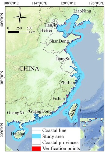
We selected China’s coastal zone as the study area, with a geographical range between 17–41°N and 107–125°E. The study area spans nine provinces (Liaoning, Hebei, Shandong, Jiangsu, Zhejiang, Fujian, Guangdong, Guangxi, Taiwan, and Hainan) and three climatic zones (temperate, subtropical, and tropical). The total length of the coastline in this area exceeds 18000 km. In addition, China has more than 6500 islands with areas greater than 500m², of which more than 400 are inhabited (Liu et al. 2019a). The vast sea area and long coastline provide innate natural conditions for the flourishing development of the mariculture industry in China. Based on the available literature and visual inspections, we empirically defined a buffer zone of 50 km from the coastline as the coastal zone (Figure 1), covering most of the mariculture areas in China.

Figure 1. Location of the study area and the spatial distribution of verification points.

Mariculture in China is of various types, including pond mariculture, cage culture, raft culture, hoisting cage culture, bottom sowing culture, and industrial culture. This study mainly focused on the types of mariculture visible at the sea surface and can be detected by satellites, including cage culture, raft culture, and hoisting cage culture. Cage culture mainly consists of cages and accessories for fixing cages, and it is primarily used for cultivating fish, crustaceans, shellfish, and other marine animals. The cage is generally woven with nylon, PVC, or other netting materials and installed on a wooden cage frame to make it float on the sea. Raft culture mainly consists of submerged ropes and floating rafts secured to the seabed by piles or anchors. The cultivated crops, such as seaweeds (e.g. kelp, Undaria pinnatifida, and laver) and oysters, are attached to the submerged ropes to grow (Hu et al. 2021). Other types of mariculture that are not visible at the sea surface, such as bottom sowing culture, were excluded from the monitoring because remote sensing cannot detect the signal reflected by targets on the seafloor. Specifically, a region was identified as mariculture areas if mariculture existed in this region within 2020, regardless of duration.

2.2. Data and preprocessing

2.2.1. Sentinel-2 and Sentinel-1 multi-temporal data

The Sentinel-2 satellites (including Sentinel-2A and Sentinel-2B) are equipped with a MultiSpectral Instrument (MSI), capable of providing optical images with a 10 m high spatial resolution. The MSI offers 13 spectral bands, including four 10 m resolution bands, i.e. B2 (Blue), B3 (Green), B4 (Red), and B8 (NIR), six 20 m resolution bands, and three 60 m resolution bands. The revisit time of the Sentinel-2 decreased from 10 to 5 days after Sentinel-2B was launched. We collected all available Level-2A Sentinel-2 data for the study area between February 2020 and February 2021 from the Google Earth Engine (GEE) platform and retained only the 10 m resolution bands. Images with less than 80% cloud cover were selected and masked by the quality assessment band (QA60) to minimize the impact of clouds. The average number of valid observations per pixel in different seasons (spring, summer, fall, and winter) was 17, 15, 17 and 17, respectively.

The Sentinel-1 satellites (including Sentinel-1A and Sentinel-1B) are C-band Synthetic Aperture Radars with a frequency of 5.405 GHz and a revisit time of 12 days (6 days for two satellites), supporting both single-polarization (VV or HH) and dual-polarization (VV + VH or HH + HV). Sentinel-1 has four operating modes: the Interferometric Wide-swath mode (IW), the Wave mode (WV), the Extra Wide-swath mode (EW), and the Strip Map mode (SM). The IW is the default mode, and it acquires data with a 250 km swath at 5 m by 20 m spatial resolution. Only single-polarization VV data were selected since the weaker penetration of the cross-polarization VH data compared to the single-polarized VV data makes it difficult to observe mariculture areas (Zhang et al. 2020). We collected all available single-polarization VV images acquired in the IW mode and Ground Range Detected (GRD) format (resampled to 10 m resolution) between February 2020 and February 2021 from the GEE platform. The Sentinel-1 data from the GEE platform have been pre-processed using the European Space Agency’s (ESA) Sentinel-1 Toolbox, including thermal noise removal, radiometric calibration, and terrain correction.

2.2.2. Auxiliary data

The global multi-scale sea-land (island) shoreline dataset (2015) was used to assist in defining our study area and interpreting the mariculture areas (Liu et al. 2019b, 2019a). This fine-scale shoreline dataset was produced through human–computer interactions based on Google Earth high-resolution satellite images, among which the area of the smallest island (reef) was 6 m². Given China’s large and diverse land cover, applying this dataset to mask land areas without mariculture could effectively reduce misclassification. On the other hand, mariculture areas far from the mainland coastline were mainly distributed around the islands, so the island (reef) shoreline data could be utilized to prevent the omission of extraction results.

The tidal flat map of China (China_Tidal Flat, CTF) was used to mask tidal flat areas in the post-processing procedure. (Jia et al. 2021). Tidal flats are transition zones between marine and terrestrial environments, including intertidal mudflats, rocks, and sands. Due to the proximity of mariculture to tidal flats in some coastal zones, they can easily be misclassified (Wang et al. 2019). The CTF map is the first 10 m spatial resolution tidal flat map covering the entire coastline of China. It is produced based on time series of Sentinel-2 images acquired in 2019 and 2020 with an overall accuracy of 95%.

The ocean bathymetry data (GEBCO_2021 grid) was used to analyse the physical environmental parameters of mariculture areas. The GEBCO_2021 grid is the latest release of the global terrain model produced by the Nippon Foundation-GEBCO Seabed 2030 Project framework, and it has a high spatial resolution of 15 arc seconds (GEBCO Bathymetric Compilation Group 2021 2021). The GEBCO_2021 is also a global seafloor topography product that provides gridded bathymetric data. However, the ocean bathymetry data extracted from the GEBCO_2021 grid are missing in some regions close to the mainland. We used an inverse distance interpolation algorithm (IDW) to interpolate the missing areas and resampled the data to a 10 m resolution.

2.3. Methods

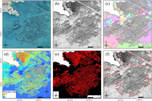
The workflow of mapping China’s offshore mariculture areas using dense time-series Sentinel-2 and Sentinel-1 data is illustrated in Figure 2. The method can be summarized into five steps: 1) generation of edge probability feature map; 2) feature map segmentation based on an improved watershed algorithm; 3) extraction of mariculture areas based on features of segmented objects; 4) generation of SAR temporal mean images; 5) morphological processing and artificial review. In Figure 3, we demonstrate the extraction process by taking the typical mariculture area in the coastal zone of Liaoning Province as an example. The details of each step are described in the following.

Figure 2. Workflow of the mariculture mapping.

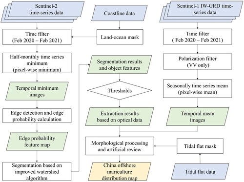
Figure 3. Example of mariculture areas extraction process in the coastal zone of Liaoning Province. (a) One of the temporal minimum images; (b) edge probability feature map; (c) segmentation results with a random color assignment to each object; (d) spectral feature map of segmented objects; (e) extraction results based on segmented object features; (f) final extraction results of mariculture areas.

2.3.1. Edge probability feature map generation

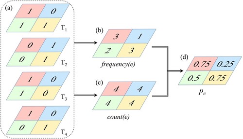
Following the Sentinel-2 data acquisition and preprocessing steps described in Section 2.2.1, twenty-four composite images were generated by applying a minimum operator along the time dimension to the preprocessed images at half-monthly intervals. Compared to the median or mean operator, the synthesis strategy using a minimum operator is more effective in reducing the effect of thin clouds that cannot be thoroughly masked by the Q60 band in the sea background. A narrow composite interval (half-month) can increase the good-quality observations of mariculture areas under different growth stages. Then, the Canny operator was used to detect the edges of mariculture areas, and the detection results were transformed into binary images (Canny 1986; Wang et al. 2019). After the edge detection of each composite image was completed, the edge probability feature map was obtained based on the formula (1). (1) $\begin{array}{c}{p}_e={\displaystyle \frac{frequency\left(e\right)}{count\left(e\right)}}\end{array}$(1) Where $p_e$ represents pixel’s value in the edge probability feature map, i.e. the edge probability value, $frequency\left(e\right)$ represents the frequency of the pixel being detected as an edge, and $count\left(e\right)$ represents the number of valid observations of the pixel. The schematic diagram of the calculation process is shown in Figure 4.

Figure 4. Schematic diagram of the calculation process of edge probability feature map. (a) Time-series optical composite images; (b) calculation results of $frequency\left(e\right)$; (c) calculation results of $count\left(e\right)$; (d) calculation results of $p_e$, i.e. the edge probability feature map.

Unlike the spectral features (e.g. NDVI), which are affected by the growth stage of the culture, mariculture areas with a rectangular shape can maintain stable edge features. Compared with the optical image (Figure 3a), the edge information of mariculture areas was highlighted in the edge probability feature map. The contrast and separability between the mariculture and non-mariculture areas were significantly enhanced (Figure 3b). We completed the above steps using the GEE platform to acquire edge probability feature maps covering the study area.

2.3.2. Feature map segmentation

An improved watershed segmentation algorithm was used to segment the edge probability feature map. This method is a two-stage technique. In the first stage, the classical watershed algorithm with a pre-improvement process was used to obtain an initial segmentation. In the second stage, the full lambda-schedule algorithm was used as a post-improvement process to merge small objects in the initial segmentation results to avoid over-segmentation (Wang et al. 2020; Wang et al. 2018a; Liu et al. 2011).

The watershed algorithm is a powerful technique for image segmentation with high accuracy in locating the edges of adjacent regions. At present, the simulated immersion algorithm proposed by Vincent and Soille (1991) is one of the most widely used methods to implement watershed segmentation. It was adopted as the watershed algorithm in this study. The specific steps of pre-segmentation are shown as follows:

(1) An edge probability feature map was smoothed using a Gaussian low-pass filter.

(2) The gradient magnitude map was calculated using the Sobel operator from the filtered feature map.

(3) To calculate the cumulative distribution function and discard the lowest 30 per cent of gradient magnitude values.

(4) To segment the reconstructed gradient map through the simulated immersion algorithm.

The watershed algorithm is sensitive to subtle changes in grayscale values. Therefore, we reconstructed the gradient magnitude map to suppress over-segmentation and reduce the computational cost of the subsequent region merging process. The choice of 30% is not critical, and a conservative value was selected because the final segmentation results were obtained after performing the full lambda-schedule algorithm. A slight over-segmentation is preferable to under-segmentation.

The full lambda-schedule algorithm is a method for the iterative merging of adjacent objects based on spectral and spatial information (Redding et al. 1999; Robinson, Redding, and Crisp 2002). A pair of adjacent objects $O_i$ and $O_j$ are merged into one object if their merging cost $t_{i,j}$ is less than a defined threshold $T$. The merging cost $t_{i,j}$ is defined as follows: (2) $\begin{array}{c}{t}_{i,j}={\displaystyle \frac{O_i\times O_j}{O_i+O_j}\times {\displaystyle \frac{{\left|\left|u_i-u_j\right|\right|}^2}{length\left(\mathrm{\partial }\left(O_i,O_j\right)\right)}}}\end{array}$(2) where $O_i$ and $O_j$are the areas of objects $i$ and $j$, $u_i$ and $u_j$ are the average value of objects $i$ and $j$, $\left|\left|u_i-u_j\right|\right|{}^2$ is the Euclidean distance between the grey values of objects $i$ and $j$, and $length\left(\mathrm{\partial }\left(O_i,O_j\right)\right)$ is the length of the common border of objects $i$ and $j$.

The specific steps of object merging are shown as follows:

1. To calculate the information of each object required in the algorithm (e.g. area, mean grey value).

2. Among all adjacent pairs of objects, find the pair $\left(i,j\right)$ with the smallest $t_{i,j}$.

3. If $t_{i,j}\le T$, objects $i$ and $j$ are merged to form object $ij$ as the new object $i$.

4. To repeat steps (2) and (3) until there is only one object, or $t_{i,j}>T$ for all adjacent pairs of objects.

The threshold ($T$) can be calculated by cumulative probability analysis. The formula is as follows: (3) $\begin{array}{c}F\left(x_a\right)=P\left(x\le T\right)=\alpha ,\left(0<\alpha <1\right)\end{array}$(3) where $x$ is the merging cost of a pair of adjacent objects, $P$ is the cumulative probability when $x\le T$, and $\alpha$ is the merging scale. In this study, the optimal merging scale was selected using the iterative “trial and error’ method (Duro, Franklin, and Dubé 2012). After a series of experiments, we finally determined that 0.9 is an optimal merging scale, which can be applicable to different scenarios. The whole image segmentation process ended after the object merging was completed. It can be found that the edge probability feature map is well segmented with high continuous and clear boundaries between mariculture and non-mariculture areas (Figure 3c).

2.3.3. Mariculture areas extraction

The mariculture areas were extracted based on features of segmented objects. Each object in the segmentation result has a unique identification, and various features can be computed for each object. To distinguish between mariculture and non-mariculture areas, we selected the spectral feature (mean grey value), geometric feature (area), and textural feature (grey-level co-occurrence matrix variance, GLCM variance) for each object. Since the edge features of mariculture areas are greatly highlighted, there should be significant differences in the mean grey value between mariculture and non-mariculture objects (Figure 3d). Three auto-thresholding techniques were tested to select the most suitable threshold for the spectral feature, including the Otsu algorithm (Otsu 1979), Moment-Preserving algorithm (Tsai 1985) and Minimum Error algorithm (Kittler and Illingworth 1986). These techniques could segment the feature image into two classes by automatically determining the optimal threshold for locating the valley between two overlapping peaks of the histogram. Specifically, the Otsu algorithm is based on optimizing an objective function that minimizes the between-class variance. The Moment-Preserving algorithm preserves the moments of the thresholded image. The Minimum Error algorithm is based on the optimization of an objective function that minimizes the average classification error rate. We finally selected the Moment-Preserving algorithm as the optimal auto-thresholding technique by comparing the classification performance of the three techniques in multiple typical regions. For the geometric feature, it is easy to notice that the area of mariculture objects has an upper and lower limit, so objects with too low or too high area values can be judged as non-mariculture objects. For the textural feature, the GLCM variance values of non-mariculture objects are significantly lower than that of mariculture objects because the interior of the non-mariculture objects is more homogeneous than mariculture objects. These two features can assist in eliminating non-mariculture objects with abnormal mean grey values. We collected a large number of samples and determined thresholds for geometric and textural features based on the statistics of their feature values (Table 1). The threshold value of 10.2 is the mean value of GLCM variance of non-mariculture area samples, which is much lower than the GLCM variance value of mariculture area samples. The extraction results of mariculture areas based on Sentinel-2 optical data are shown in Figure 3(e).

Table 1. Object features for mariculture areas extraction.

Feature	Threshold	Description
Mean gray value	Dynamically determined by the Moment-Preserving algorithm	Mean value of gray values for pixels within each object
Area	(60, 290000)	Total number of pixels within each object
GLCM variance	10.2	Mean value of GLCM variance values for pixels within each object

2.3.4. Composition of temporal mean SAR images

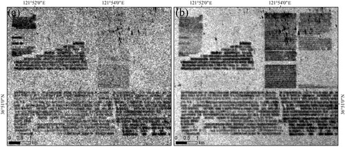
The Sentinel-1 time-series data was used to assist in visually inspecting extraction results based on Sentinel-2 data in the subsequent post-processing step. First, the single-polarization VV images acquired using the steps described in Section 2.2.1 were calculated as mean-value composite images according to the specified periods. Here, we selected five time periods: spring (Feb 2020 to May 2020), summer (May 2020 to Aug 2020), fall (Aug 2020 to Nov 2020), winter (Nov 2020 to Feb 2021), and the whole year (Feb 2020 to Feb 2021). Then, a focal median filter was applied to sharpen the edges and remove more noise (Ottinger, Clauss, and Kuenzer 2017). Compared with the original images, the mean-value composite images reduced the impact of speckle noises and enhanced the backscattering of mariculture areas. In addition, the seasonal composite image can dramatically improve the visual recognition of mariculture areas with specific growth periods and prevent the omission of mariculture areas with short breeding cycles (Figure 5).

Figure 5. Comparison of SAR images before and after composition. (a) One of the original time series images, and (b) one of the temporal mean images.

2.3.5. Morphological processing and artificial review

Post-processing procedures were necessary to modify and improve the resultant mariculture areas. First, the tidal flat areas were masked based on the CTF map because they might be misclassified due to their proximity to mariculture areas. Then, the morphological closing operation was used to fill the internal area of mariculture areas to resolve the boundary non-closure. Reflected signals from mariculture areas in some coastal zones are difficult to capture by optical sensors. SAR data has a more significant capability than optical data in monitoring their distribution (Fan et al. 2018; Fu et al. 2019a; Fu et al. 2021). Therefore, the composite SAR images obtained in 2.3.4 were visually interpreted to supplement and correct the mariculture areas that were not accurately identified from the optical data. Artificial review using optical data-based extraction results as reference data can establish expert knowledge to ensure the accuracy and integrity of the extraction results. After the above steps, the final extraction results of mariculture areas were obtained (Figure 3f).

3. Results

3.1. Accuracy assessment

For the simplicity of data processing, the study area was equally split into 110 tiles with a size of 1 degree in latitude and longitude. The edge probability feature maps covering the study area were processed tile by tile. Ultimately, a complete offshore mariculture distribution map of China was obtained by merging the extraction results of each tile (Figure 6A). The extraction results of some typical zones are shown in Figure 6(a1-d3).

Figure 6. Spatial distribution of tiles with a size of 1 degree in latitude and longitude and the final mariculture distribution map of China (A). (a1-a3) The optical image, edge probability feature map, and extraction results of coastal zones in Shandong Province; (b1-b3) optical image, edge probability feature map, and extraction results of coastal zones in Jiangsu Province; (c1-c3) optical image, edge probability feature map, and extraction results of coastal zones in Fujian Province; and (d1-d3) optical image, edge probability feature map, and extraction results of coastal zones in Guangdong Province.

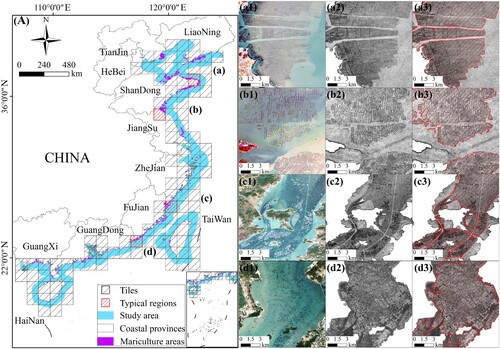
We used the random sampling method to evaluate the accuracy of the mariculture extraction results. First, 700 verification points in mariculture areas and 300 verification points in non-mariculture areas were generated by the random sampling tool in ArcGIS 10.8. Figure 1 shows the spatial distribution of verification points in the study area. The validation points were then imported into Google Earth and overlaid with high-resolution images to obtain the actual ground class attribute of each point. Since the number of images in the same area within a year in Google Earth is generally 1–2 scenes, the acquisition date of these images is random, which is very likely inconsistent with the existence time of the mariculture. Therefore, the verification points judged non-aquaculture needed to be superposed with the mean value composite SAR images for secondary judgment to acquire their actual attributes. Finally, a confusion matrix was calculated, including the User Accuracy (UA), Producer Accuracy (PA), Overall Accuracy (OA), and kappa coefficient (Table 2). We implemented the bootstrapping method to evaluate the uncertainty level of the accuracy (Efron and Tibshirani 1997; Duan et al. 2020). Bootstrapping was executed with 1,000 iterations, with the mean of the distribution used for estimates and 95% quantile for confidence intervals.

Table 2. Error matrix for the mariculture and non-mariculture classes.

		Ground truth points
	Class	Mariculture	Non-mariculture
Map points	Mariculture	644	4
	Non-mariculture	56	296
Producer Accuracy (PA)		92.00%
User Accuracy (UA)		99.38%
Overall Accuracy (OA)		94.00%
Kappa coefficient		0.91

The results of the accuracy and uncertainty level assessment indicate that the mariculture extraction results obtained in this study have high accuracy, with an overall accuracy of 94.00% (91.80–96.00%, 95% confidence interval), a user accuracy of 99.38% (98.50–100.00%, 95% confidence interval) and a producer accuracy of 92.00% (89.40–94.90%, 95% confidence interval).

3.2. Spatial and area distributions of mariculture in China in 2020

3.2.1. Distribution of mariculture in different provinces

Figure 7(a) shows the distribution of China’s offshore mariculture in 2020. According to the classification results, the total area of mariculture in China was approximately 1173249.22 ha. In addition, mariculture (712887.51 ha) in the northern provinces (Shandong, Hebei, and Liaoning) covers significantly larger than in the southern provinces (460361.71 ha), accounting for 60.76% of the total area. There were also notable differences in the mariculture areas in the different provinces (Figure 7b, c). Specifically, Shandong had the largest mariculture area (458642.06 ha), accounting for 39.09% of the total area in China, followed by Fujian (151877.91 ha) and Liaoning (144106.72 ha). The mariculture in these three provinces accounted for more than half of the country’s mariculture, reaching 64.32%. Jiangsu, Guangdong, and Hebei’s mariculture were roughly equivalent, ranging from 110138.73 ha to 120475.15 ha. Mariculture in Zhejiang, Hainan, and Taiwan was the smallest, accounting for only 6.11% of the total area.

Figure 7. Extraction results of the mariculture areas in China’s coastal zones. (a) Spatial distribution of China’s mariculture (mariculture is displayed using 30 km × 30 km grids); (b) statistics of the mariculture area in China’s coastal provinces; and (c) proportions of the mariculture area in China’s coastal provinces.

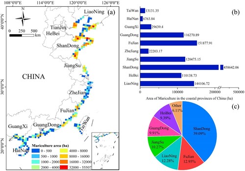
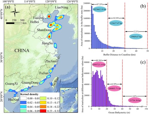
To present a more explicit spatial perspective, we employed kernel density estimation to calculate the density level of the mariculture in each raster cell by assessing neighborhood variation (Dehnad 1987). The kernel density tool with a 50 km search radius in ArcGIS 10.8 was used to generate a density map, which provides an intuitive and visual understanding of the spatial distribution pattern of mariculture. We observed that the mariculture in China presented an obvious spatial distribution characteristic of ‘Denser North and Sparser South’ and was concentrated in four key regions: the Shandong coastal area, the southern coastal area of Liaodong Peninsula, the Hebei coastal area, and the Fujian coastal area (Figure 8a). Shandong had the broadest coverage of mariculture, with a high concentration of mariculture areas along the entire coast. In particular, although Hebei Province ranked fourth in the area of mariculture, it had the highest kernel density, indicating the highest spatial aggregation of mariculture.

Figure 8. Spatial distribution pattern of China’s offshore mariculture. (a) Kernel density analysis map; (b) distribution of mariculture at different distances from coastline; and (c) distribution of mariculture at different ocean depths.

3.2.2. Distribution of mariculture within the proximity of the coastline

The area of mariculture within the proximity of different buffer distances from the coastline was obtained via buffer analysis and overlay analysis. We gradually increased the buffer distance at 1 km intervals, and the mariculture area in each buffer zone segment with a buffer distance from 1 km to 50 km was calculated. As shown in Figure 8(b), about 98% of mariculture was distributed within 30 km of the coastline, and very little mariculture was distributed beyond 30 km from the coastline. In general, mariculture was most concentrated within 15 km of the coastline, where the cumulative area increased rapidly from 19.23% to 87.25% with increasing distance. In addition, the mariculture within different buffer segments varied greatly, ranging from 225560.95 ha to 16792.19 ha, among which the buffer zone 1 km from the coastline had the largest coverage. In the region 15–30 km from the coastline, the mariculture area of each buffer zone segment rapidly decreased, accounting for only 10.54% of the total area.

3.2.3. Distribution of mariculture at different ocean depths

We applied the tabulate area tool in ArcGIS 10.8 to calculate the mariculture area at different ocean depths. As shown in Figure 8(c), the mariculture was mostly concentrated in the region with water depths less than 20 m, accounting for 89.56% of the total area. The mariculture in the region with water depths of 20–40 only accounted for 8.59%. Moreover, mariculture was rarely distributed in regions with water depths greater than 40 m. Unlike the distribution of mariculture varying with distance from the coastline (as the distance from the coastline increased, the mariculture decreased rapidly), mariculture did not exhibit a regular change in the region with water depths of 1–20 m. However, in regions with water depths of 20–40 m, mariculture decreased drastically from 29801.92 ha to 1256.36 ha with increasing water depth.

4. Discussion

4.1. Comparison with previous studies

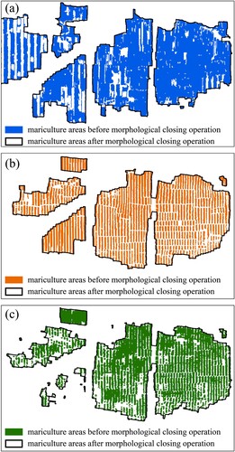
There are two relevant studies: one was conducted by Liu et al. (2020) based on Landsat 8 data in 2018, referred to here as the Landsat 8-derived dataset, and the other was conducted by Fu et al. (2021) based on GF-1 data in 2019, referred to here as the GF-1-derived dataset. The study area (excluding Taiwan coastal zone) and extracted mariculture types of these two studies were the same as this study. In addition, the targets extracted in these two studies are independent mariculture individuals. However, the targets extracted in this study are contiguous mariculture patches. Therefore, the extraction results of these two studies were processed using the morphological closing operation to make the results more comparable (Figure 9).

Figure 9. Schematic diagram of morphological closing operation processing. (a) Mariculture areas from this study before and after the morphological closing operation; (b) mariculture areas from the Landsat 8-derived dataset before and after the morphological closing operation; and (c) mariculture areas from the GF-1-derived dataset before and after the morphological closing operation.

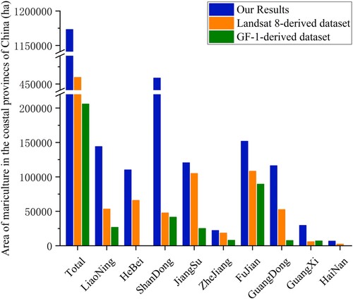
The comparison of different study results is shown in Figure 10. Regarding the total area of mariculture in China, the Landsat 8-derived dataset and the GF-1-derived dataset were 459595.70 and 205920.28 ha, respectively, which are substantially lower than the result of our study (1173249.22 ha). As for the spatial distribution pattern, our results show that mariculture was centralized in the coastal zones of the northern provinces (Shandong, Hebei, and Liaoning), accounting for 60.76% of the total area. In contrast, the Landsat 8-derived dataset and GF-1-derived dataset indicate that the mariculture was mainly distributed in the southern provinces, and only about 35% of the mariculture was distributed in the northern provinces. In terms of the area of mariculture in different provinces, the results obtained in our study are significantly larger than those of the other two studies. In addition, the area extracted from the Landsat 8-derived dataset was also significantly larger than that extracted from the GF-1-derived dataset. For example, in our study, the most extensive coverage of mariculture was in Shandong Province (458642.06 ha), followed by Fujian Province (151877.91 ha). However, the Landsat 8-derived dataset and GF-1-derived dataset showed that Fujian Province had the most extensive coverage of mariculture (108211.5 and 89501.74 ha, respectively), and Shandong Province had less than 50000 ha. For Hebei Province, our results and the Landsat 8-derived dataset showed the presence of large mariculture areas in its coastal zones (110138.73 and 65942.94 ha, respectively), but the GF-1-derived dataset showed that there was almost no mariculture in the coastal zones of Hebei Province. Hainan Province also has the same situation as Hebei Province. In addition, the area of mariculture in Liaoning Province and Guangdong Province derived from the GF-1-derived dataset were also lower (26772.92 and 7604.33 ha, respectively), which was about 1/2 and 1/7 of Landsat 8-derived dataset, and about 1/5 and 1/15 of our results. The area of mariculture in Zhejiang Province and Jiangsu Province derived from the Landsat 8-derived dataset were extremely close to our results, which were significantly larger than the results of the GF-1-derived dataset.

Figure 10. Statistics on the mariculture area of China’s coastal provinces from different studies.

4.2. Advantage of applying time-series and multi-source remote sensing data

There are two common features concerning the remote sensing data used in the two previous studies mentioned above. First, they used single-view images rather than time-series images. Second, they only used the optical data without combining other remote sensing data. As seen from the comparison of the results presented in Section 4.1, our study identified many previously undetected mariculture areas, which could be explained by the advantages of using time-series data and multi-source remote sensing data fusion.

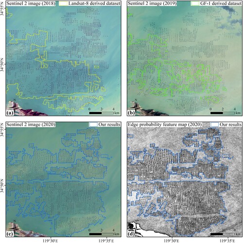
First, mariculture is significantly affected by marine environmental factors such as the water depth, water temperature, salinity, pH, and dissolved oxygen concentration. Due to the large span of China’s coastlines from east to west (over 1500 km) and from north to south (over 2500 km), the mariculture in different geographical locations has distinct temporal and spatial differences in terms of the culture types and breeding cycles. Mariculture in different regions generally possesses unique phenological properties. Some mariculture may only exist for a few specific months. In addition, the types of mariculture may rotate depending on seasonal transitions in the same region, making it difficult to cover all of them using a single-view image. Taking Jiangsu Province as an example (Figure 11), the spatial distribution of mariculture areas in its coastal zones was basically consistent from 2018 to 2020. After the Landsat 8-derived dataset (Figure 11a) and the GF-1-derived dataset (Figure 11b) were overlaid on the optical images, it was found that both of their extraction results had substantial omissions. However, no apparent omissions were found in our extraction results based on time-series data (Figure 11c). Therefore, omissions due to incomplete coverage of images are inevitable when using single-view images for mariculture extraction. The application of edge probability feature maps based on time-series optical data can effectively improve the integrity of the extraction results (Figure 11d).

Figure 11. Comparison of the extraction results from different studies in coastal zones of Jiangsu Province. (a) Results from the Landsat 8-derived dataset and the optical image from 2018; (b) results from the GF-1-derived dataset and the optical image from 2019; (c) our results and the optical image from 2020; and (d) our results and the corresponding edge probability feature map.

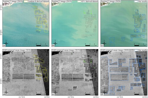
Second, the detection of mariculture based on passive optical remote sensing data should be able to obtain the reflected signal of the target. However, there are numerous mixed pixels in the mariculture areas because the sea surface constantly changes with wave fluctuations, which makes it difficult for the optical image to completely and accurately obtain the reflected signal, especially for submerged mariculture areas. SAR, an active microwave sensor, emits electromagnetic waves that can penetrate clouds, fog, and seawater. Due to the weak echo energy of seawater and the strong echo energy of mariculture areas (e.g. floating rafts, bases, fences, and cages), the backscattering characteristics of mariculture targets are more obvious. Therefore, there are significant tonal differences and contrasts between the mariculture areas and seawater background in SAR images, which enables the identification of the mariculture area. Taking the southern coastal zone of Shandong Province as an example (Figure 12), the previous two studies and our extraction method based on optical data failed to completely extract the mariculture areas in this region (Figure 12a–c). After comparing composite SAR images from 2018 to 2020, it was found that large mariculture areas existed in this region all year round (Figure 12d–f). However, most mariculture areas were not evident in the edge probability feature map, which means they could not be effectively identified using the optical data (Figure 12c). The reason may be that these mariculture areas were often submerged in seawater, making it difficult for passive remote sensing to acquire their reflected signals. Thus, by performing an integrated judgment based on multi-source remote sensing data, our method is capable of discovering mariculture areas under various environmental conditions.

Figure 12. Comparison of the extraction results from different studies in coastal zones of Shandong Province. (a) Results from the Landsat 8-derived dataset and the optical image from 2018; (b) results from the GF-1-derived dataset and the optical image from 2019; (c) extraction results based on optical data in our study and the optical image from 2020; (d) results from the Landsat 8-derived dataset and the composite SAR image from 2018; (e) results from the GF-1-derived dataset and the composite SAR image from 2019; and (f) final extraction results based on optical and SAR data in our study and the composite SAR image from 2020.

4.3. Potential of using remote sensing-derived datasets for mariculture production estimation

Sustainable food from the sea and sustainable economic utilization of marine resources are the specific goals of Sustainable Development Goal 14 (SDG 14) (United Nations Global Compact and the World Business Council for Sustainable Development 2015). Therefore, dynamic and objective data about mariculture production are essential for reaching SDG 14. However, due to the inconsistency of statistical standards and data acquisition limitations, it is often difficult to obtain detailed, consistent and comparable global mariculture production statistics (Ottinger, Clauss, and Kuenzer 2018). Therefore, estimating mariculture production based on remote sensing observations will be a crucial objective for future studies on coastal zone management and sustainable development of the marine economy, which can fill the gaps of non-reporting and incomplete-reporting regions or countries.

The mariculture production statistics for China’s coastal provinces in 2019 and 2020 were collected (The Editor Committee of China Fishery Statistical Yearbook 2019, 2020; Fisheries Bureau of Taiwan 2020). We observed that the official production statistics and remote sensing-derived mariculture area revealed a highly corresponding trend at the provincial level, with an R² of 0.78 (Figure 13a). Provinces with a large remote sensing-derived mariculture area also showed a high level of mariculture production in the official statistics. This close and solid correlation confirms the potential of estimating mariculture production based on the area acquired by remote sensing observations and further verifies the accuracy of our results. However, the mariculture production statistics did not exhibit significant correlations with the area calculated from the Landsat 8-derived dataset and the GF-1-derived dataset, which may be primarily due to the incompleteness of their results (Figure 13b, c).

Figure 13. Regression analysis between province-wise official production statistics and (a) the mariculture area calculated in this study; (b) the mariculture area calculated from the Landsat 8-derived dataset; (c) the mariculture area calculated from the GF-1-derived dataset.

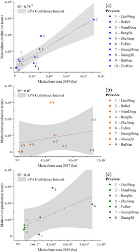
Only the mariculture in Hebei, Jiangsu, and Fujian provinces exhibited a rather large inconsistent trend compared to the production statistics. Taking Fujian Province as an example, Fujian is the province with the highest production of oysters and kelp in China. In 2019, the production of oysters and kelp accounted for 39.41% and 15.73%, respectively, of its total mariculture production. The oyster species cultured in Fujian Province mainly include Crassostrea angulata, Crassostrea gigas, and Crassostrea hongkongensis, which have high growth rates and short culture cycles compared with other animal species. With the support of advanced breeding technology such as the oyster–kelp–seaweed integrated multi-trophic mariculture model, the total production per unit area is quite high, which may weaken the linear relationship between production and area (Wartenberg et al. 2017). Therefore, further consideration of various factors such as culture type, breeding cycles, seawater temperature, and seabed sediments is required to improve the accuracy and robustness of the production estimation model in the future.

4.4. Uncertainties and limitations in mariculture mapping

Accurate mapping of mariculture areas on a national scale is challenging. There are still some potential uncertainties and limitations in this study. First, despite the short revisit interval of Sentinel-2, it is almost impossible to capture clear images containing complete mariculture areas throughout the year due to complex sea conditions and cloudy weather. Therefore, artificial review based on composite SAR images remains a necessary supplement to the results extracted based on optical data. This could explain, for example, why large mariculture areas in the coastal zones of Shandong Province were not identified in previous studies. Second, although the QA60 band method was used to remove clouds in this study, the overall cloud detection effect of this method was unstable, which affected the identification of mariculture areas. Third, although most mariculture areas are distributed in semi-enclosed bays or shallow seas where waves are attenuated, the influence of waves still cannot be ignored. The edge features of mariculture areas were extracted based on instantaneously captured images. Great waves may significantly change the position of mariculture areas, which weakens the stability of edge probability features, especially for mariculture areas far from the shoreline. Fourth, the latest shoreline dataset with high accuracy was used for land-sea separation in our method, but there are still some newly expanded aquaculture ponds or land in the study area. In addition, high turbidity seawater near coastlines or estuaries could be misclassified as mariculture areas. These misclassifications required manual correction in the post-processing step to improve the extracted results. Given the advantages of SAR with all-weather operation capability, it is necessary to focus on extracting mariculture areas based on the feature-level fusion of optical and SAR data in future work.

5. Conclusions

The acquisition of accurate and comprehensive spatial distribution data for mariculture is the key first step in supporting scientific management of the mariculture industry and sustainable development of the marine economy. In this study, aiming at the problems (e.g. small research scales, single data sources, and the high possibility of omissions) in previous studies, we developed a method of extracting the mariculture areas on a national scale using dense time-series optical data and SAR data. The overall accuracy reached 94.00% (91.80–96.00%, 95% confidence interval), and the kappa coefficient was 0.91. The results show that the total area of mariculture in China in 2020 was 1173249.22 ha, among which Shandong, Fujian, and Liaoning provinces had the most extensive coverage, accounting for more than 60% of the total area. In terms of the spatial distribution pattern of mariculture, mariculture in China presented an obvious spatial distribution characteristic of ‘Denser North and Sparser South’. In addition, mariculture was most concentrated in the regions within 30 km of the coastline and at water depths less than 40 m, accounting for 87.25% and 89.56%, respectively, of the total area.

Compared with previous studies, our results provide new knowledge and a better understanding of the spatial distribution of mariculture in China’s coastal zones. By performing an integrated judgment based on multi-source remote sensing data, large areas of previously undetected mariculture were discovered, which considerably filled the gaps in the existing datasets, especially in Shandong, Hebei, and Taiwan provinces. In addition, our results indicate that mariculture areas obtained by remote sensing observations have significant potential for estimating production. Further analysis and evaluation of the water quality parameters (e.g. suspended solids, chlorophyll-a concentration, and turbidity), physical environmental parameters (e.g. water depth, current velocity, and sea surface temperature), and socio-economic parameters (e.g. distance to the coastline, distance to industries, and distance to cities) can be carried out in the future. These researches will provide references for mariculture production estimation, site selection, and spatial planning around the world and can contribute to the sustainable development of the global marine economy.

Data availability statement

The Sentinal-2 and Sentinal-1 data that support the findings of this study are available at [https://developers.google.com/earth-engine/datasets]; The global multi-scale sea-land (island) shoreline dataset (2015) that support the findings of this study are available at [http://www.geodoi.ac.cn/WebCn/doi.aspx?Id = 1265]; The tidal flat map of China (China_Tidal Flat, CTF) that support the findings of this study are available at [http://www.geodata.cn/data/datadetails.html?dataguid = 192951013633169&docid = 1315]; The ocean bathymetry data GEBCO_2021 grid that support the findings of this study are available at [https://www.gebco.net/data_and_products/gridded_bathymetry_data/].

Disclosure statement

No potential conflict of interest was reported by the author(s).

Additional information

Funding

This work was supported by the National Key Research and Development Program of China [grant number 2021YFB3900501], the National Natural Science Foundation of China [grant number 41671436; 41901354; 41890854] and the Innovation Project of LREIS [grant number O88RAA01YA].

References

- Alleway, H. K., C. L. Gillies, M. J. Bishop, R. R. Gentry, S. J. Theuerkauf, and R. Jones. 2019. “The Ecosystem Services of Marine Aquaculture: Valuing Benefits to People and Nature.” BioScience 69 (1): 59–68. doi:10.1093/biosci/biy137.
- Campbell, B., and D. Pauly. 2013. “Mariculture: A Global Analysis of Production Trends Since 1950.” Marine Policy 39: 94–100. doi:10.1016/j.marpol.2012.10.009.
- Canny, J. 1986. “A Computational Approach to Edge Detection.” IEEE Transactions on Pattern Analysis and Machine Intelligence PAMI-8 (6): 679–698. doi:10.1109/TPAMI.1986.4767851.
- Costello, C., L. Cao, S. Gelcich, MÁ Cisneros-Mata, C. M. Free, H. E. Froehlich, C. D. Golden, et al. 2020. “The Future of Food from the sea.” Nature 588 (7836): 95–100. doi:10.1038/s41586-020-2616-y.
- Dehnad, K. 1987. “Density Estimation for Statistics and Data Analysis.” Technometrics 29 (4): 495. doi:10.1080/00401706.1987.10488295.
- Duan, Y., X. Li, L. Zhang, D. Chen, S. A. Liu, and H. Ji. 2020. “Mapping National-Scale Aquaculture Ponds Based on the Google Earth Engine in the Chinese Coastal Zone.” Aquaculture 520: 734666. doi:10.1016/j.aquaculture.2019.734666.
- Duarte, C. M., A. Bruhn, and D. Krause-Jensen. 2022. “A Seaweed Aquaculture Imperative to Meet Global Sustainability Targets.” Nature Sustainability 5: 185–193. doi:10.1038/s41893-021-00773-9.
- Duro, D. C., S. E. Franklin, and M. G. Dubé. 2012. “A Comparison of Pixel-Based and Object-Based Image Analysis with Selected Machine Learning Algorithms for the Classification of Agricultural Landscapes Using SPOT-5 HRG Imagery.” Remote Sensing of Environment 118: 259–272. doi:10.1016/j.rse.2011.11.020.
- The Editor Committee of China Fishery Statistical Yearbook. 2019. China Fishery Statistical Yearbook (2019). Beijing: China Agriculture Press. https://cafs.ac.cn/info/1397/34095.htm (Accessed 1 January 2022).
- The Editor Committee of China Fishery Statistical Yearbook. 2020. China Fishery Statistical Yearbook (2020). Beijing: China Agriculture Press. https://cafs.ac.cn/info/1397/37342.htm (Accessed 1 January 2022).
- Efron, B., and R. Tibshirani. 1997. “Improvements on Cross-Validation: The 632+ Bootstrap Method.” Journal of the American Statistical Association 92 (438): 548–560. doi:10.1080/01621459.1997.10474007.
- Fan, J., J. Chu, J. Geng, and F. Zhang. 2015. “Floating Raft Aquaculture Information Automatic Extraction Based on High Resolution SAR Images.” 2015 IEEE International Geoscience and Remote sensing symposium (IGARSS), 3898-3901.
- Fan, J., X. Wang, X. Wang, X. Liu, J. Zhao, and Q. Meng. 2019. “GF-3 PolSAR Marine Aquaculture Recognition Based on Complex Convolutional Neural Networks.” 2019 tenth International Conference on intelligent control and information processing (ICICIP), 112-115.
- Fan, J., J. Zhao, D. Song, X. Wang, X. Wang, and X. Su. 2018. “Marine Floating Raft Aquaculture Dynamic Monitoring Based on Multi-Source GF Imagery.” 2018 7th International Conference on agro-geoinformatics (agro-geoinformatics), 1-4.
- FAO. 2018. The State of World Fisheries and Aquaculture 2018 - Meeting the Sustainable Development Goals. http://fao.org/documents/card/zh/c/I9540EN/ (Accessed 1 January 2022).
- FAO. 2020. The State of World Fisheries and Aquaculture 2020 - Sustainability in Action (Accessed 1 January 2022).
- Fisheries Bureau of Taiwan, China. 2020. Taiwan, China Fishery Statistical Yearbook (2020). https://fa.gov.tw/index.php (Accessed 1 January 2022).
- Fu, Y., J. Deng, H. Wang, A. Comber, W. Yang, W. Wu, S. You, Y. Lin, and K. Wang. 2021. “A new Satellite-Derived Dataset for Marine Aquaculture Areas in China's Coastal Region.” Earth System Science Data 13 (5): 1829–1842. doi:10.5194/essd-13-1829-2021.
- Fu, Y., J. Deng, Z. Ye, M. Gan, K. Wang, J. Wu, W. Yang, and G. Xiao. 2019a. “Coastal Aquaculture Mapping from Very High Spatial Resolution Imagery by Combining Object-Based Neighbor Features.” Sustainability 11 (3): 637. doi:10.3390/su11030637.
- Fu, Y., Z. Ye, J. Deng, X. Zheng, Y. Huang, W. Yang, Y. Wang, and K. Wang. 2019b. “Finer Resolution Mapping of Marine Aquaculture Areas Using WorldView-2 Imagery and a Hierarchical Cascade Convolutional Neural Network.” Remote Sensing 11 (14): 1678. doi:10.3390/rs11141678.
- Gebco Bathymetric Compilation Group 2021. 2021. The GEBCO_2021 Grid - a Continuous Terrain Model of the Global Oceans and Land. NERC EDS British Oceanographic Data Centre NOC. doi:10.5285/c6612cbe-50b3-0cff-e053-6c86abc09f8f.
- Geng, J., J. Fan, and H. Wang. 2017. “Weighted Fusion-Based Representation Classifiers for Marine Floating Raft Detection of SAR Images.” IEEE Geoscience and Remote Sensing Letters 14 (3): 444–448. doi:10.1109/LGRS.2017.2648641.
- Hu, Y., J. Fan, and J. Wang. 2017. “Target Recognition of Floating Raft Aquaculture in SAR Image Based on Statistical Region Merging.” 2017 seventh International Conference on information Science and Technology (ICIST).
- Hu, F., H. Zhong, C. Wu, S. Wang, Z. Guo, M. Tao, C. Zhang, et al. 2021. “Development of Fisheries in China.” Reproduction and Breeding 1 (1): 64–79. doi:10.1016/j.repbre.2021.03.003.
- Jia, M., Z. Wang, D. Mao, C. Ren, C. Wang, and Y. Wang. 2021. “Rapid, Robust, and Automated Mapping of Tidal Flats in China Using Time Series Sentinel-2 Images and Google Earth Engine.” Remote Sensing of Environment 255: 112285. doi:10.1016/j.rse.2021.112285.
- Kittler, J., and J. Illingworth. 1986. “Minimum Error Thresholding.” Pattern Recognition 19 (1): 41–47. doi:10.1016/0031-3203(86)90030-0.
- Li, H., X. Li, Q. Li, Y. Liu, J. Song, and Y. Zhang. 2017. “Environmental Response to Long-Term Mariculture Activities in the Weihai Coastal Area, China.” Science of the Total Environment 601-602: 22–31. doi:10.1016/j.scitotenv.2017.05.167.
- Liang, P., S.-C. Wu, J. Zhang, Y. Cao, S. Yu, and M. H. Wong. 2016. “The Effects of Mariculture on Heavy Metal Distribution in Sediments and Cultured Fish Around the Pearl River Delta Region, South China.” Chemosphere 148: 171–177. doi:10.1016/j.chemosphere.2015.10.110.
- Liu, C., R. Shi, Y. Zhang, Y. Shen, J. Ma, L. Wu, W. Chen, et al. 2019. “2015: How Many Islands (Isles, Rocks), How Large Land Areas and How Long of Shorelines in the World? ——Vector Data Based on Google Earth Images.” Journal of Global Change Data & Discovery 3 (02): 124–148. doi:10.3974/geodp.2019.02.03.
- Liu, C., R. Shi, Y. Zhang, Y. Shen, J. Ma, L. Wu, W. Chen, et al.. 2019a. Global Multi-Scale sea-Land (Island) Shoreline Dataset Based on Google Earth Remote Sensing Images (2015). Global Change Research Data Publishing & Repository. doi:10.3974/geodb.2019.04.13.V1
- Liu, H., and J. Su. 2017. “Vulnerability of China’s Nearshore Ecosystems Under Intensive Mariculture Development.” Environmental Science and Pollution Research 24 (10): 8957–8966. doi:10.1007/s11356-015-5239-3.
- Liu, Y., Z. Wang, X. Yang, Y. Zhang, F. Yang, B. Liu, and P. Cai. 2020. “Satellite-based Monitoring and Statistics for Raft and Cage Aquaculture in China’s Offshore Waters.” International Journal of Applied Earth Observation and Geoinformation 91: 102118. doi:10.1016/j.jag.2020.102118.
- Liu, L., X. Wen, A. Gonzalez, D. Tan, J. Du, Y. Liang, W. Li, et al. 2011. “An Object-Oriented Daytime Land-fog-Detection Approach Based on the Mean-Shift and Full Lambda-Schedule Algorithms Using EOS/MODIS Data.” International Journal of Remote Sensing 32 (17): 4769–4785. doi:10.1080/01431161.2010.489067.
- Lu, Y., W. Shao, and J. Sun. 2021. “Extraction of Offshore Aquaculture Areas from Medium-Resolution Remote Sensing Images Based on Deep Learning.” Remote Sensing 13 (19): 3854. doi:10.3390/rs13193854.
- Lulijwa, R., E. J. Rupia, and A. C. Alfaro. 2020. “Antibiotic use in Aquaculture, Policies and Regulation, Health and Environmental Risks: A Review of the top 15 Major Producers.” Reviews in Aquaculture 12 (2): 640–663. doi:10.1111/raq.12344.
- Meng, W., and R. A. Feagin. 2019. “Mariculture is a Double-Edged Sword in China.” Estuarine, Coastal and Shelf Science 222: 147–150. doi:10.1016/j.ecss.2019.04.018.
- Naylor, R. L., R. W. Hardy, A. H. Buschmann, S. R. Bush, L. Cao, D. H. Klinger, D. C. Little, J. Lubchenco, S. E. Shumway, and M. Troell. 2021. “A 20-Year Retrospective Review of Global Aquaculture.” Nature 591 (7851): 551–563. doi:10.1038/s41586-021-03308-6.
- Otsu, N. 1979. “A Threshold Selection Method from Gray-Level Histograms.” IEEE Transactions on Systems, Man, and Cybernetics 9 (1): 62–66. doi:10.1109/TSMC.1979.4310076.
- Ottinger, M., K. Clauss, and C. Kuenzer. 2017. “Large-Scale Assessment of Coastal Aquaculture Ponds with Sentinel-1 Time Series Data.” Remote Sensing 9 (5): 440. doi:10.3390/rs9050440.
- Ottinger, M., K. Clauss, and C. Kuenzer. 2018. “Opportunities and Challenges for the Estimation of Aquaculture Production Based on Earth Observation Data.” Remote Sensing 10 (7): 1076. doi:10.3390/rs10071076.
- Redding, N., D. Crisp, D. Tang, and G. N. Newsam. 1999. “An efficient algorithm for Mumford-Shah segmentation and its application to SAR imagery. Digital Image Computing: Techniques and Applications (DICTA-99), Perth, 35–41.
- Robinson, D. J., N. Redding, and D. Crisp. 2002. Implementation of a fast algorithm for segmenting SAR imagery. Defence Science Technology Organisation, Australia. https://researchgate.net/publication/27254411_Implementation_of_a_fast_algorithm_for_segmenting_SAR_imagery (Accessed 1 January 2022).
- Shi, T., Q. Xu, Z. Zou, and Z. Shi. 2018. “Automatic Raft Labeling for Remote Sensing Images via Dual-Scale Homogeneous Convolutional Neural Network.” Remote Sensing 10 (7): 1130. doi:10.3390/rs10071130.
- Sun, Z., J. Luo, J. Yang, Q. Yu, L. Zhang, K. Xue, and L. Lu. 2020. “Nation-Scale Mapping of Coastal Aquaculture Ponds with Sentinel-1 SAR Data Using Google Earth Engine.” Remote Sensing 12 (18): 3086. doi:10.3390/rs12183086.
- Tsai, W.-H. 1985. “Moment-preserving Thresolding: A new Approach.” Computer Vision, Graphics, and Image Processing 29 (3): 377–393. doi:10.1016/0734-189X(85)90133-1.
- United Nations Global Compact and the World Business Council for Sustainable Development. 2015. Conserve and sustainably use the oceans, seas and marine resources for sustainable development. https://sdgcompass.org/sdgs/sdg-14/ (Accessed 1 January 2022).
- Vincent, L., and P. Soille. 1991. “Watersheds in Digital Spaces: An Efficient Algorithm Based on Immersion Simulations.” IEEE Transactions on Pattern Analysis and Machine Intelligence 13 (6): 583–598. doi:10.1109/34.87344.
- Wang, M., Q. Cui, J. Wang, D. Ming, and G. Lv. 2017. “Raft Cultivation Area Extraction from High Resolution Remote Sensing Imagery by Fusing Multi-Scale Region-Line Primitive Association Features.” ISPRS Journal of Photogrammetry and Remote Sensing 123: 104–113. doi:10.1016/j.isprsjprs.2016.10.008.
- Wang, Y., Q. Meng, Q. Qi, J. Yang, and Y. Liu. 2018a. “Region Merging Considering Within- and Between-Segment Heterogeneity: An Improved Hybrid Remote-Sensing Image Segmentation Method.” Remote Sensing 10 (5): 781. doi:10.3390/rs10050781.
- Wang, Y., Q. Qi, L. Jiang, and Y. Liu. 2020. “Hybrid Remote Sensing Image Segmentation Considering Intrasegment Homogeneity and Intersegment Heterogeneity.” IEEE Geoscience and Remote Sensing Letters 17 (1): 22–26. doi:10.1109/LGRS.2019.2914140.
- Wang, J., L. Sui, X. Yang, Z. Wang, Y. Liu, J. Kang, C. Lu, F. Yang, and B. Liu. 2019. “Extracting Coastal Raft Aquaculture Data from Landsat 8 OLI Imagery.” Sensors 19 (5): 1221. doi:10.3390/s19051221.
- Wang, Z., X. Yang, Y. Liu, and C. Lu. 2018b. “Extraction of Coastal Raft Cultivation Area with Heterogeneous Water Background by Thresholding Object-Based Visually Salient NDVI from High Spatial Resolution Imagery.” Remote Sensing Letters 9 (9): 839–846. doi:10.1080/2150704X.2018.1468103.
- Wartenberg, R., L. Feng, J. J. Wu, Y. L. Mak, L. L. Chan, T. C. Telfer, and P. K. S. Lam. 2017. “The Impacts of Suspended Mariculture on Coastal Zones in China and the Scope for Integrated Multi-Trophic Aquaculture.” Ecosystem Health and Sustainability 3 (6): 1340268. doi:10.1080/20964129.2017.1340268.
- Xu, Y., Z. Hu, Y. Zhang, J. Wang, Y. Yin, and G. Wu. 2021. “Mapping Aquaculture Areas with Multi-Source Spectral and Texture Features: A Case Study in the Pearl River Basin (Guangdong), China.” Remote Sensing 13 (21): 4320. doi:10.3390/rs13214320.
- Yu, J., W. Yin, and D. Liu. 2020. “Evolution of Mariculture Policies in China: Experience and Challenge.” Marine Policy 119: 104062. doi:10.1016/j.marpol.2020.104062.
- Zhang, Y., C. Wang, Y. Ji, J. Chen, Y. Deng, J. Chen, and Y. Jie. 2020. “Combining Segmentation Network and Nonsubsampled Contourlet Transform for Automatic Marine Raft Aquaculture Area Extraction from Sentinel-1 Images.” Remote Sensing 12 (24): 4182. doi:10.3390/rs12244182.
- Zheng, Y., J. Wu, A. Wang, and J. Chen. 2018. “Object- and Pixel-Based Classifications of Macroalgae Farming Area with High Spatial Resolution Imagery.” Geocarto International 33 (10): 1048–1063. doi:10.1080/10106049.2017.1333531.