Routeview: an intelligent route planning system for ships sailing through Arctic ice zones based on big Earth data

ABSTRACT

The potential of Arctic routes (ARs) has attracted global attention, and exploiting the Arctic has become an important strategy for many countries. However, there are still some challenges for ships sailing in Arctic ice zones, including harsh marine environments and the insufficient service capacity of sea ice information service systems. To better understand the route changes in the Arctic and extract real-time ship navigation routes, we developed an online interactive route planning system (RouteView) for ships sailing in the Arctic based on big Earth data. RouteView includes two main features: (1) an online calculation interface is provided for optimal routes along the Arctic Northeast Passage (NEP) 60 days into the future by utilizing reinforcement learning (RL) based on sea ice and meteorological data, and (2) an online ice-water classification is established based on synthetic aperture radar (SAR) data and deep learning to help users extract the sea ice distribution in real time. This work can potentially enhance the safety of shipping navigation along the NEP and improve information extraction methods for ARs.

KEYWORDS:

• Arctic northeast passage
• information extraction system
• reinforcement learning
• U-Net
• route planning
• ice-water classification

1. Introduction

In recent decades, the Arctic has warmed two to three times as fast as the global rate due to the unique features in the Arctic climate system – a phenomenon known as Arctic amplification (Fang et al. 2022; Blackport and Screen 2020; Dai et al. 2019; Cohen, Pfeiffer, and Francis 2018). A warmer Arctic has been driving reductions in Arctic sea ice. For example, the sea ice extent decreased at a rate of – 4.0% every 10 years during the recent period of 2007–2020 (Thoman, Richter-Menge, and Druckenmiller 2020). The accelerating sea ice melt in the Arctic is opening up new polar shipping routes, such as the Northeast Passage (NEP) from the Pacific to the Northern Atlantic, along the Norwegian and Russian Arctic coasts. Compared with the traditional Suez Canal route, the NEP will shorten the journey by 40% and the sailing time by approximately 20 days (Yumashev et al. 2017; Zhu, Cao, and Ai 2018), thus creating a potential alternative route for global trade.

Although Arctic routes (ARs) serve as shortcuts for shipping in northern Europe and North America and have created many opportunities for the shipping industry, there are still some challenges for ships sailing in Arctic ice zones. First, some factors, such as large ice caps, icebergs, ice floes, snowstorms and low temperatures, are unfavorable for ship navigation and pose considerable navigation risks (Buixadé Farré et al. 2014). Moreover, many ice zones in the Arctic are not equipped with sufficient aid for navigation, leading to insufficient rescue capabilities (Christodoulou et al. 2022; Aase and Jabour 2015). Additionally, many excellent data sharing systems (Li et al. 2021; Pan et al. 2021; Li et al. 2020) have been developed to provide information services. However, the information service capabilities of these systems are still limited. For example, these systems mainly rely on the traditional method of manual experience plus metadata keywords to provide data retrieval and download services, resulting in a large amount of spatiotemporal information that cannot be obtained by users. Moreover, these shared data are difficult to directly apply in ship navigation planning, and technicians must often perform further manual processes to extract more valuable ship planning information; however, this approach is generally time consuming, laborious and costly. Finally, most of the research on Arctic navigation has focused on the analysis of historical route distributions (Chen et al. 2019) and their future changes (Chen et al. 2021). These cases can illustrate the overall distribution trends and patterns of ARs, but in actual navigation planning, more time-sensitive indicators are needed, such as the optimal route distribution over the next 60 days for different ships, sea ice concentrations (SICs) along optimal routes, sea ice thicknesses (SITs) along optimal routes and temperatures along optimal routes. At present, none of these indicators along the NEP are calculated online to meet the relevant user requirements.

To extract valuable information for Arctic navigation in a timely manner, we developed an interactive online navigation information extraction system called RouteView. This new system, which integrates data, algorithms, and scalable computation, is intended to make breakthroughs in the automation of AR information services and lessen technical barriers to navigation analysis by utilizing open-source web services and cloud storage technologies. This article contributes to the literature in three major respects.

1. From the perspective of computational procedure, a flexible interactive planning system is developed for navigation routes along the NEP based on reinforcement learning (RL), which helps users quickly compute the shortest and most secure daily navigation route for different types of ships between an origin and a destination 60 days into the future.

2. From the perspective of both remote sensing and big data, a convolutional network for image segmentation (U-Net) is integrated into our system based on the Big Earth Data Cloud Service Platform (BEDCSP), and online interactive ice-water classification for ARs is provided, which helps users extract sea ice at a high resolution and in real time.

3. From the perspective of visualization, a CesiumJS-based toolbox is developed for the three-dimensional (3D) visualization and processing of complex computing tasks, thus providing an intuitive and friendly user interface.

The remainder of this article is organized as follows. Section 2 discusses related studies. Section 3 presents the system design and capabilities. Section 4 provides two web applications of RouteView. Evaluation and validations for two important algorithms are then introduced in Section 5. Finally, a detailed discussion and conclusions are presented in Section 6 and Section 7, respectively.

2. Related studies

In this section, the current status of route information extraction methods for Arctic ice zones and some existing information systems (ISs) related to the Arctic are reviewed.

2.1. Route information extraction methods for Arctic ice zones

Planning a safe and reasonable route for different ships involves the consideration of many factors, including not only hydrological, meteorological, economic and political factors but also relevant implicit conditions, such as the operational ability and psychological quality of crew members, crew health, port supply and the emergency rescue capacity. In this paper, we focus on how Arctic ships can safely sail under the influence of hydrological and meteorological factors from the perspective of climate change. Therefore, ‘route information’ is considered from two perspectives: ① analysis of optimal navigation routes in Arctic ice zones at the macrolevel and ② extraction of sea ice information in local sea areas. In this section, the relevant research progress is introduced.

Pathfinding is to find a path with different objective functions, like distance, estimated time of arrival (ETA) and fuel consumption. The Dijkstra algorithm (Dijkstra 1959), A* algorithm (Hart, Nilsson, and Raphael 1972) and ant colony algorithm (ACA) (Dorigo, Birattari, and Stutzle 2006) are traditional, widely used pathfinding algorithms. We summarize the application cases of these three algorithms for AR planning in Table 1. These algorithms have been successfully used to identify an optimal route that best meets certain criteria (the shortest, least costly, fastest, etc.) between two points in a large network.

Table 1. Typical pathfinding algorithms for Arctic routes.

Algorithm	Year	Main functions (Literature)	Characteristics
Dijkstra	2013	The algorithm calculated the optimal routes based on simulated sea ice and environmental data in the Arctic (Nam et al. 2013).	The running environment of the algorithm requires global map information to determine the best path. If the map is too large and there are many vertices, the execution efficiency level is low. The Dijkstra algorithm will always find the most optimal route for the two-dimensional and static routing problem.
	2016	The algorithm found the most economically efficient routes with the minimal possible ice thickness using graph modification and the Dijkstra algorithm (Zvyagin and Voitkunskaia 2016).
	2019	A fuzzy analytic hierarchy process (FAHP), an extended version of the Dijkstra algorithm, was developed to help ship management teams determine the optimal route for safe, short and economic navigation (Şahin 2019).
A*	2017	To reduce the occurrence of collision accidents, a route planning was used for ice-going ships based on a modified A∗ algorithm under multiconstraint conditions (Zhang et al. 2017).	The A* algorithm is a generalization of Dijkstra's algorithm that cuts down on the size of the subgraph that must be explored. If the influence of the heuristic part is set to be very low, the A* algorithm also can find global solution.
	2018	A new ice navigation system with a modified A* path planning algorithm called the HFS-A* algorithm was developed to solve the multicriteria decision-making problem in Arctic route planning (Wang, Zhang, and Qian 2018).
ACA	2018	ACA combined with a genetic algorithm (GA) was used to model living organism optimization behavior to perform efficient ship route planning in transoceanic crossing (Tsou and Cheng 2013).	ACA optimizes a problem by having an updated pheromone trail and moving these ants around in the search space according to simple mathematical formulae over the transition probability and total pheromone in the region (Ahmed et al. 2020).
	2019	The improved ACA was adopted to solve the optimum energy efficiency route planning problem in ice-covered water (Zhang et al. 2019).
	2021	The novel double ant colony algorithm (NDACA) based on dynamic feedback was utilized to identify the lowest-energy-consumption route (Dong et al. 2021).

In contrast to these traditional methods, RL enables an agent to learn autonomously in an interactive environment by trial and error using feedback from its own actions and experiences. The goal is to find a suitable action model that maximizes the total cumulative reward of the agent. Mnih et al. (2015) believes that combining RL with pathfinding is equivalent to allowing agents to combine learning abilities similar to the way humans find solutions. In 2006, the proposal of deep learning (Hinton and Salakhutdinov 2006) successfully promoted the vigorous development of deep RL. The core idea is to consider complex environmental characteristics based on the powerful perceptual ability provided by deep learning and to implement an intelligent decision-making analysis process that combines RL and environmental interactions. In 2015, Google's DeepMind team launched the deep Q-network (DQN) and noted that deep RL has reached a decision analysis level commensurate with that of humans (Volodymyr et al. 2015). Two years later, the team launched AlphaGo and defeated Li Shishi, the world champion of Go. After that, AlphaGo Zero based on deep RL defeated AlphaGo after a short period of training without aid based on human experience (Silver et al. 2017).

At present, RL has achieved good performance in the fields of gaming (Lample and Chaplot 2017), intelligent transportation systems (Haydari and Yilmaz 2020), autonomous driving (Sallab et al. 2017) and recommendation systems (Tang et al. 2019), but relevant applications to AR planning do not exist.

2.2. Sea ice information extraction methods for local sea areas

SIC and SIT are key components of the polar climate system, and SIC and SIT in local sea areas are the main factors affecting the navigation of ships (Shyu and Ding 2016; Zhao et al. 2022). At present, sea ice products mainly originate from passive microwave remote sensing. However, the current resolution of these sea ice products mostly ranges from 4 to 25 km, which cannot meet actual navigation needs. Therefore, higher-resolution synthetic aperture radar (SAR) images should be utilized to extract sea ice information, overcome the disadvantages of low-resolution passive microwave sensors and the influence of clouds on optical images, and significantly improving the accuracy of sea ice monitoring (Lyu, Huang, and Mahdianpari 2022; Mäkynen et al. 2014).

Information extraction in the era of remote sensing data (Zhang et al. 2021; Wang et al. 2022) is characterized by data-driven information analysis models, and deep learning currently provides the best algorithm for this approach (Reichstein et al. 2019) Deep learning involves the use of a hierarchical architecture designed by stacking several blocks composed of filters (or layers) with specific functions to capture the information in images. Among the available deep learning networks, convolutional neural networks (CNNs) are the most popular and commonly applied to analyze remote sensing images (Li, Huang, and Gong 2019). Many researchers have employed CNNs to improve the accuracy and efficiency of sea ice classification based on SAR data. Wang, Andrea Scott, and Clausi (2017) used a CNN trained with image analysis graphs to estimate ice concentrations from SAR imagery acquired over the Gulf of Saint Lawrence. The authors’ results showed that the CNN could generate ice concentration estimates with improved detail and accuracy relative to Arctic Radiation and Turbulence Interaction Study (ARTIST) SIC products, but the CNN was less sensitive to pixel-level details than was a multilayer perceptron (MLP). Xu and Andrea Scott (2017) adopted the CNN-based AlexNet model as a feature extractor to conduct sea ice and water classification with SAR imagery. This method performed quite well, with an overall classification accuracy of 92.36% on average. Gao et al. (2019) proposed a transferred multilevel fusion network (MLFN) for sea ice change detection from SAR images, representing the first time that transferred deep learning was applied for sea ice change detection. David et al. (2021) developed a CNN architecture to generate Arctic sea ice products from Sentinel-1 SAR data combined with Advanced Microwave Scanning Radiometer 2 (AMSR2) data. From the authors’ experiments, it was concluded that CNNs are suitable for multisensor fusion, even with sensors that differ in resolution; however, the noisy first subswath of the Sentinel-1 sensor was not reduced. By utilizing the advantages of CNNs for depth feature extraction, Han et al. (2021) designed a deep learning network structure for SAR and optical images and achieved sea ice image classification through feature extraction and the feature-level fusion of heterogeneous data.

These CNN-based models can achieve the end-to-end classification of sea ice and open water based on SAR images. However, most of these CNN-based models used an image classification framework (Mikołajczyk and Grochowski 2018) and not a pixel-level segmentation framework (Minaee et al. 2021). To address the defects of traditional CNN classification, Long, Shelhamer, and Darrell (2015) proposed fully convolutional networks (FCNs) to recover the category of each pixel from general features. Each network realizes end-to-end segmentation, but the segmentation results are typically not sufficiently detailed. Inspired by FCNs and encoder-decoder models, U-Net was developed to yield more precise segmentations with fewer training images (Ronneberger, Fischer, and Brox 2015). Although initially developed for the semantic segmentation of biomedical images, U-Net has been successfully applied in sea ice detection. To highlight the advantages of artificial intelligence (AI) applications for sea ice classification, Li et al. (2020) constructed a generalized AI framework based on U-Net. The authors acquired six Sentinel-1 SAR images to detect sea ice or water in the Bering Strait and found that the proposed U-Net-based model was capable of detecting sea ice from SAR images at the pixel level. Radhakrishnan, Scott, and Clausi (2021) utilized U-Net to obtain SIC estimates from horizontal transmit – horizontal receive (HH) – and horizontal transmit – vertical receive (HV)-polarized SAR images. Their results showed that using U-Net proved superior to employing the traditionally used CNNs, as it eliminated shortcomings seen in previous models for ice concentration estimation, including computational efficiency, accuracy, dependence on patch size, etc. Ren et al. (2021) integrated a dual-attention mechanism (position and channel attention modules) into the original U-Net model to extract more characteristic features. Their experiments showed that the improved model could effectively achieve pixel-level classification with SAR images. These studies verified that U-Net is an effective framework for sea ice information mining from remote sensing imagery.

2.3. Information systems for the Arctic

Currently, ISs related to the Arctic mainly focus on sea ice data sharing and shipping route visualization. This section mainly reviews the status of Arctic ISs from these two perspectives.

Many government agencies and institutions worldwide provide sea ice information through online ISs. Table 2 provides a partial summary of sea ice ISs based on web mapping, including the spatiotemporal data coverage and types of maps and links. These systems provide access not only to specific sea ice data but also to various levels of ice maps. In terms of ice mapping, Li, Xiong, and Ou (2011) classified three kinds of web maps: static raster image maps (SRMs), raster images with animation maps (RAMs), and two-dimensional (2D) vector maps (2DVMs). As shown in Table 2, some systems provide SRMs representing ice conditions, and others are gradually beginning to use virtual globes (VGs) to display sea ice data. Almost all data sharing services provide abundant SIC data, which can be downloaded in near real time (the last three days). However, near-real-time SIT data during the Arctic summer navigation period are basically unavailable, which makes navigation route analyses of ships highly uncertain, especially for key sea areas with complex ice conditions.

Table 2. ISs for sea ice (last accessed on July 1, 2022). ‘ – ’ indicates nonsupport.

No.	Dataset	Data source	Temporal coverage	Spatial coverage	Frequency	Map type	Link
1	MASIE-AMSR2 SIC	NSIDC	2012 to present	Northern Hemisphere	1 d	SRMs	https://nsidc.org
2	Global SIC (SSMIS)	OSI SAF	Last 31 days	Global	1 d	SRMs	https://osi-saf.eumetsat.int
3	Global SIC (AMSR-2)	OSI SAF	Last 31 days	Global	1 d	SRMs	https://osi-saf.eumetsat.int
4	CryoSat-2 SIT	NSIDC	2010 to present	Northern Hemisphere	30 days	VG	https://nsidc.org
5	SMOS SIT	SMOS	2010 to present	Northern Hemisphere	7 days	–	https://smos-diss.eo.esa.int
6	ATLAS/ICESat-2 Sea Ice Freeboard	NSIDC	2018 to present	Global	91 days	VG	https://nsidc.org
7	EASE-Grid Sea Ice Age	NSIDC	1984–2020	Northern Hemisphere	7 days	–	https://nsidc.org

The abbreviations used in Table 2 are defined as follows:

MASIE: Multisensor Analysed Sea Ice Extent.

AMSR2: Advanced Microwave Scanning Radiometer 2.

NSIDC: the National Snow & Ice Data Center, which is a United States information and referral center in support of polar and cryospheric research.

OSI SAF: the Satellite Application Facility on Ocean and Sea Ice, which is a project led by Météo France, the Norwegian Meteorological Institute, the Danish Meteorological Institute, Ifremer and the Royal Netherlands Meteorological Institute (KNMI).

SMOS: Soil Moisture and Ocean Salinity, which is one of the European Space Agency's Earth Explorer missions that provides science and research information for the Living Planet Programme.

ATLAS: the Advanced Topographic Laser Altimeter System.

Some early efforts have focused on using web-based geographic information systems (GISs) to facilitate better visualization of Arctic shipping routes in recent years. The Center for High North Logistics (CHNL, https://arctic-lio.com/) provides Arctic transportation and logistical data based on a 2D map (Gunnarsson 2013), but this information can only be updated periodically by the system administrator. Based on a 3D GIS, PolarGo, developed at Wuhan University in China, can achieve the visual fusion of information related to polar investigation, research and policy in China and other countries. The program can overlay real-time and historical ship navigation data layers to provide data support for decision-makers (http://x.hbaa.cn/Long/). These types of data analysis and visualization based on a 3D GIS are becoming increasingly common. Chang et al. (2015) developed a route planning system using Google Earth. Additionally, Wu et al. (2022) built an advanced ship navigation information service system (SNISS) based on a 3D GIS. The two systems are route display systems based on VGs. The former manually calculates the navigation route, and the latter uses an automatic calculation process, but neither provides a calculation interface for human-computer interactions; therefore, users cannot extract route information in real time according to their own needs. Information extraction systems (Mirończuk 2018; Kang et al. 2017) integrated with data, algorithms, and scalable computations are currently the best ways for researchers to achieve efficient big data analysis; however, at present, no information extraction systems are being applied to ARs.

3. System design and capabilities

RouteView is an online interactive information extraction system for ARs based on CesiumJS (https://cesium.com/platform/cesiumjs/), and it combines the functionalities of many Python software packages. RouteView has evolved in the past three years through many iterations, with the most-recent available version being V3.0; the aim is to transform large volumes of data into valuable knowledge through online computation.

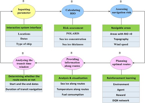
RouteView adopts a loosely coupled strategy that separates data collection, computation and visualization into three individual modules. As shown in Figure 1, the data model encompasses various types of raw remote sensing data, such as Sentinel, sea ice product and meteorological data. We develop automatic data collection and processing middleware to automatically process these data.

Figure 1. Flowchart of the modular big data framework of RouteView.

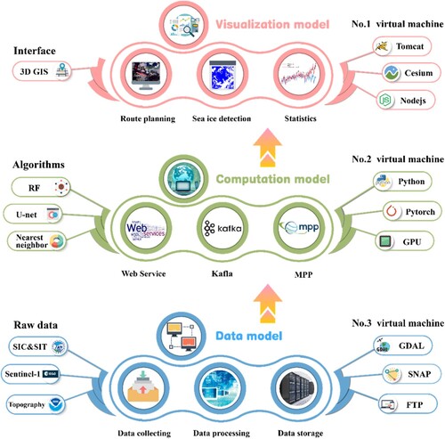
The computation model transforms raw data into the final valuable ‘information’. To reduce the complexity of information extraction, all algorithms and models, such as the pathfinding algorithm and ice-water classification model, are transformed into WebService format and deployed in BEDCSP (http://english.casearth.com/index.php).

The visualization model provides an interactive interface for users through a 3D GIS, achieving the real-time calculation of the optimal route under different constraints and online automated sea ice-water classification. To improve the user’s experience, Cesium, Canvas, Web Graphics Language (WebGL), Asynchronous JavaScript and Extensible Markup Language (AJAX) and other technologies are employed to enhance visualization effects.

A flow chart of the different steps involved in information extraction through RouteView is summarized in Figure 1 and is subsequently described in further detail below.

3.1. Data model

The data model involves data collection, processing and warehousing, which are automatically performed each day to provide important data guarantees for the online and real-time calculations of users. Moreover, a massive parallel processing (MPP) database (Wu, Guo, and Yang 2020) is utilized to store the data and analysis results. In this section, we mainly introduce the characteristics of the data used in the system and the corresponding automatic processing steps.

3.1.1. Data characteristics

The SIC, SIT, temperature and wind speed used for route analysis in our system were automatically obtained from the Flexible Global Ocean-Atmosphere-Land System Model, finite volume version 2 (FGOALS-f2), a subseasonal to seasonal climate prediction system (Li et al. 2021). FGOALS-f2 can be used to obtain daily predictions (including SIT and SIC, temperature and wind speed) for the next 60 days (updated daily) at a nominal spatial resolution of 1° and was developed at the State Key Laboratory of Numerical Modeling for Atmospheric Sciences and Geophysical Fluid Dynamics (LASG), Institute of Atmospheric Physics (IAP), Chinese Academy of Sciences (CAS). Since 2018, FGOALS-f2 has been used in the dynamic model sequence of the Sea Ice Prediction Network (SIPN) Arctic sea ice distribution prediction project many times, and its prediction skills rank among the best provided (https://atmos.uw.edu/sipn/Evaluation.html). Moreover, oceanic bathymetry was derived from the Earth Topography Two Minute Gridded Elevation (ETOPO1) dataset (https://www.ngdc.noaa.gov).

For sea ice detection, Sentinel-1 (S1) data were used in our system. S1 has four operational modes: strip map (SM), interferometric wide swath (IW), extra wide swath (EW) and wave (WV) modes. The EW data have a wide coverage (400 km swath) and a short revisit period (less than 1 d at the North Pole); hence, they are suitable for monitoring polar regions. The EW data are typically provided in single-look complex (SLC) or ground-range-detected (GRD) format. The Level-1 GRD product is a multilook product and projected to the ground range using an Earth ellipsoid model. The moderate resolution product (GRDM) is a Level-1 GRD product that provides a pixel spacing of 40 m × 40 m; two other products are available at different resolutions. In this study, we used GRDM data with HH and HV polarizations to detect sea ice because these are the most frequently used modes in polar regions due to the favorable combination of coverage and resolution levels. In addition, HH polarization has a stronger signal and is less affected by additive noise than are other polarizations (Khaleghian et al. 2021) and HV polarization is less sensitive to the incidence angle and to wind. Hence, compared to single-polarization data, dual-polarization data (HH and HV) can be more effectively used to identify sea ice and sea water.

3.1.2. Data processing

For the SIC, SIT, temperature and wind speed data from FGOALS-f2, there are differences in resolution and the number of grid points; thus, the requirements of matrix operations cannot be met. To solve these problems, these data were first converted into regular grid data (the grid points were equally spaced) utilizing the nearest-neighbor method (Jegou, Douze, and Schmid 2011). Then, the daily risk index outcomes (RIOs) for different ships (e.g. merchant and Polar Class 1 (PC1) ships) in the Arctic were calculated based on the polar operational limit assessment risk indexing system (POLARIS) (Stoddard et al. 2017). The output was a GeoTiff with a 256-row by 720-column format, and each grid was associated with a different RIO indicating the risk level of a specific ship when sailing in an area covered by a certain sea ice type. Namely, a positive RIO indicated an acceptable level of risk for a certain ship in a certain area, and a negative RIO indicated an increased level of risk for the same type of ship. Finally, the Geospatial Data Abstraction Library (GDAL) (Jegou, Douze, and Schmid 2011) was used to extract the boundaries of navigable areas where RIO > 0, wind speed < 20 m/s, temperature > – 1°C (the threshold values of wind speed and temperature were empirical values set based on the recommendations of the Polar Research Institute of China), and terrain < – 13 m (Xu and Yang 2020).

Spatiotemporal analyses of remote sensing data are often performed with GIS applications, such as the Environmental Systems Research Institute’s Aeronautical Reconnaissance Coverage Geographic Information System (ESRI’s ArcGIS). Although very powerful, this tool cannot realize automatic processing and is not open-source software. Currently, the Sentinel Application Platform (SNAP) (Delgado et al. 2019) developed by the European Space Agency (ESA) offers excellent capabilities in sequential image analysis with the Image Processing Toolbox. More importantly, the functionality of SNAP can be extended via plugins that can be browsed and installed through a user interface. In this study, the SNAP toolkit written in Python was used as middleware to process S1 data, and the steps included thermal noise removal, speckle filtering, radiometric calibration, grid geolocation, linear to decibel value (dB) transformation, and feature extraction, such as for the gray-level cooccurrence matrix (GLCM; details are given in Section 3.2.2).

3.2. Computation model

The computation module transforms processed data into the final valuable ‘information’. In this section, the two most important submodules of the computation module are presented, and they are optimal route analysis and ice-water classification.

3.2.1. Optimal route analysis

Compared to the existing SNISS (Wu et al., 2021), our new system achieves significant improvements in information extraction, especially in terms of human-computer interaction. Users can derive five indicators for ship navigation in the Arctic according to their own set conditions, including optimal navigation routes for different ships, SICs along optimal routes, SITs along optimal routes, temperatures along optimal routes and transit time windows. These derived indicators can also be presented in a VG, such as Cesium. This online calculation capability can quickly enhance the navigation decision analyses of users for ships in the Arctic.

The workflow of the proposed route analysis process is automated, with six major processing steps:

Step 1: Inputting the parameters.

Users select or input the calculation parameters (e.g. the longitude and latitude of the starting and ending points, dates and types of ships)

Step 2: Calculating the risk index outcome.

The daily RIO for different ships is automatically calculated from POLARIS each day (details are given in Section 3.1).

Step 3: Extracting navigable areas.

We define the regions in which the RIO is greater than zero as navigable areas, where ships can navigate safely. These navigable areas are extracted by our system each day, which ensures the safety of navigation and provides an important basis for the online extraction of route information. The automatic processing of these regions in advance can effectively improve the efficiency of online calculations.

Step 4: Optimal route planning.

Within these navigable areas, we further plan the shortest route from the user-defined start point to the end point based on RL. This process mainly involves environment and algorithm design for RL, as shown in Figure 2.

Figure 2. Optimal route extraction based on RL.

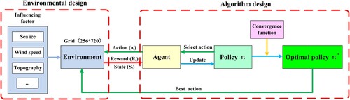
① Environmental design

We describe the Arctic environment with grids, and each grid includes navigation risk (RIO) and air temperature, wind speed and terrain information. The grids are then classified into navigable (one) and unnavigable (zero) grids. Navigable grids are areas in which RIO > 0, wind speed < 20 m/s, temperature > – 1°C and terrain < – 13 m. Similarly, grids that do not meet these conditions are defined as unnavigable grids.

To find the shortest path in navigable areas, we designed a reward function (Equation 1(2) $Q_{\pi }\left(s,a\right)=E\left[\sum _{k=0}^{\mathrm{\infty }}{\gamma }^k{R}_{t+k+1}|S_t=s,A_t=a\right]$(2) ) to guide agents to learn the environment. Once the reward function is determined, the reward value of each state will not change, and the reward value of each state reached by the agent is different. (1) $\mathrm{R}={\displaystyle \frac{dis\left(Cur,Start\right)-k\ast dis\left(Cur,End\right)}{dis\left(Start,End\right)}-1}$(1) Cur represents the current coordinate point of the agent, Start represents the starting coordinates, End represents the ending coordinates, and dis represents the European distance between two points. $\mathrm{d}\mathrm{i}\mathrm{s}\left(\mathrm{C}\mathrm{u}\mathrm{r},\mathrm{E}\mathrm{n}\mathrm{d}\right)-\mathrm{k}\ast \mathrm{d}\mathrm{i}\mathrm{s}\left(\mathrm{C}\mathrm{u}\mathrm{r},\mathrm{E}\mathrm{n}\mathrm{d}\right)$ indicates that the farther the agent is from the starting point and the closer it is to the end point, the greater the reward is, and k = 2 indicates that the reward weight of the end point is higher than that of other points. The dividend $\mathrm{d}\mathrm{i}\mathrm{s}\left(\mathrm{S}\mathrm{t}\mathrm{a}\mathrm{r}\mathrm{t},\mathrm{E}\mathrm{n}\mathrm{d}\right)$ is used to normalize the reward to prevent the training process from converging too slowly if the reward is too high. Subtracting 1 from the overall formula makes the reward constant negative, thus allowing the training process to converge faster.

② Algorithm design

We use the DQN (Mnih et al. 2015) to explore the optimal route. In the training process, the current state ($S_t$) of the agent is first input into the Q network to obtain the Q values (Equation 2(3) $\pi \left(a|s\right)=\{\begin{array}{c}{\displaystyle \frac{1-ϵ}{\left|A\left(s^{\ast }\right)\right|}+{\displaystyle \frac{ϵ}{\left|A\left(s\right)\right|}ifa=argma{x}_{a}Q\left(s,a\right)}}\\ {\displaystyle \frac{ϵ}{\left|A\left(s\right)\right|}ifa\ne argma{x}_{a}Q\left(s,a\right)}\end{array}$(3) ) corresponding to all actions (four actions: up, down, left and right); an action is then selected according to the $ϵ$-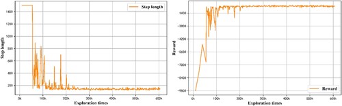greedy strategy (Equation 3). Next, all parameters, such as the current state, action, reward, and new state (S, A, R, and S’, respectively), are stored in the experience buffer pool. When all 20 interactive explorations are completed for the agent and environment, 256 samples are randomly selected from the experience pool to update the network parameters. By updating the Q values, the Q network optimizes its own parameters and converges. We use the changes in the step size and reward in each agent training stage to determine whether the network converges. If step sizes and rewards are no longer promoted, the continuous training strategy will not improve, which means that the training process ends. In Figure 3, both the step size and reward in each agent round tend to be stable after 10 min of training (after 200k steps), indicating that the network converges. At this time, we can obtain a series of optimal actions (maximum Q values) using a greedy strategy (as the number of training rounds increases, $ϵ$ gradually decreases to 0, and the $ϵ$-greedy strategy becomes a greedy strategy). These optimal actions are used to determine the optimal routes that we need to calculate. (2) $Q_{\pi }\left(s,a\right)=E\left[\sum _{k=0}^{\mathrm{\infty }}{\gamma }^k{R}_{t+k+1}|S_t=s,A_t=a\right]$(2) where $R_t$ represents the reward that the agent receives when performing action $A_t$ in state $S_t$at time t; $\gamma$ is the discount factor; ${\gamma }^k$ is used to represent the influence of action $A_t$ on the value function at time t + k; and $E$ represents the expectation. (3) $\pi \left(a|s\right)=\{\begin{array}{c}{\displaystyle \frac{1-ϵ}{\left|A\left(s^{\ast }\right)\right|}+{\displaystyle \frac{ϵ}{\left|A\left(s\right)\right|}ifa=argma{x}_{a}Q\left(s,a\right)}}\\ {\displaystyle \frac{ϵ}{\left|A\left(s\right)\right|}ifa\ne argma{x}_{a}Q\left(s,a\right)}\end{array}$(3) $ϵ$ represents the probability of random actions, $\left|\mathrm{A}\left(s\right)\right|$represents the number of selectable actions, and $\left|\mathrm{A}\left({\mathrm{s}}^{\ast }\right)\right|$ represents the number of optimal actions (generally, this number is 1). We apply $ϵ$ =  0.2; hence, the agent randomly selects an action with a probability of 0.05 ($0.2/4=$0.05), and the probability of selecting the optimal action is 0.85 ($(1-0.2)+0.2/4=0.85$).

Figure 3. Changes in the step size and reward in each round of training. (left) Change in the step size. If the end point has not been found when the step length of a round reaches 1500, the agent will start exploring again. Before 60k steps, the environmental step is 1500, indicating that the agent continues to learn the optimization strategy in this stage and has not reached the destination. From steps 60-200k, the length of the round decreases and considerably changes, indicating that once the agent has reached the destination, it will continue to learn and optimize the strategy. After 200k, the number of steps basically remains at a low level and does not change further, indicating that the agent strategy has achieved convergence. (right) Change in the reward. In steps 0-60k, the reward continues to rise, which means that although the agent has not reached the end point, it is also constantly optimizing the strategy to approach the end point. In steps 60-200k, the reward changes greatly, which means that updating strategy changes greatly in this period. After 200k, the reward is stable, indicating that the network has achieved convergence. This process is consistent with the change in the step size.

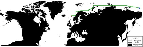
The trained DQN model can predict the optimal AR within 1 s by inputting any starting point and ending point. The green line in Figure 4 is an autopredicted optimal route of ordinary merchant ships in the Arctic on July 15th, 2013.

Figure 4. Autopredicted optimal route of ordinary merchant ships in the Arctic on July 15, 2020. The red dot is the starting point, the blue dot is the end point, and the green line represents the optimal navigation route. Black areas are unnavigable areas, and white areas are navigable areas. This graph is automatically generated by our system.

Step 5: Providing auxiliary information along the optimal routes.

The optimal route calculated in the previous step is composed of a series of coordinate points. Therefore, the corresponding SIC, SIT and temperature along the NEP can be queried from the MPP database using the nearest-neighbor method and displayed in a 3D chart. In addition, the fuel cost associated with traveling the optimal routes is calculated according to a shipping profit model (Xu and Yang 2020).

Step 6: Analyzing the transit time window.

If our system can find a route with fixed start and end points within navigable areas along the NEP (according to the navigation conditions of merchant ships) on a particular day, the NEP is considered safely navigable on that day. In this study, the optimal transit route of the NEP (Mulherin, Sodhi, and Eppler 1999) from the Kara to Bering Straits (the start and end points) is used to determine whether the NEP is navigable on a certain day. On this basis, we can calculate the duration of transit navigation as well as the first (start) and last (end) dates of NEP transit navigation.

For the functionalities corresponding to each step mentioned above, we harness WebService to encapsulate them in the independence and replaceability modules. This modular architecture (Figure 5) allows us to update each module independently and conveniently. Steps 2 and 3 are important data preparation stages, steps 4 and 5 are the core parts of online user calculations, and step 6 is the expansion of the route planning function of the system, which can be used to automatically analyze the number of days the NEP is navigable in a certain year. All steps are automatically completed by our system.

Figure 5. Six core modules of optimal automatic route extraction with WebService.

3.2.2. Ice-water classification

The route planning method mentioned in the previous section mainly analyses optimal shipping routes in the Arctic region during the summer navigation period, and its spatial resolution is low (approximately 100 km). For key sea areas, a sea ice distribution map with high spatial resolution can be obtained by remote sensing satellites, which can provide reliable and fine ice condition services for Arctic ships. Additionally, this information provides a supplement to the macrodistribution of ARs.

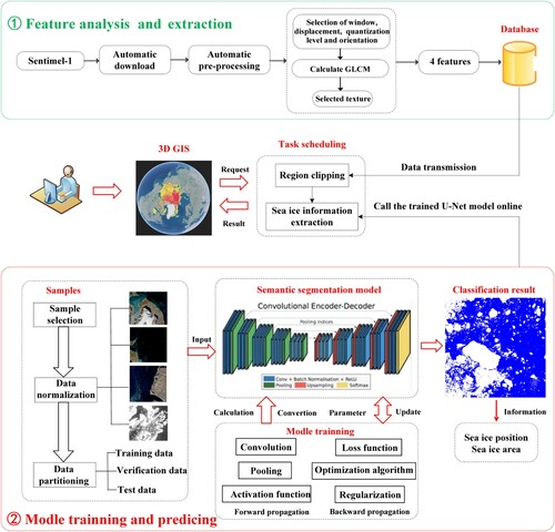
RouteView applies a deep learning model with a U-Net architecture, a well-known FCN for pixel-level segmentation, to classify sea ice and open water from SAR images. This architecture is not dependent on patch size and can make predictions with fine details and limited noise. There are two core steps in this automated classification process: (i) feature analysis and extraction and (ii) model training and prediction (Figure 6). These steps are further described below.

Figure 6. Two main processes of online sea ice detection with the U-Net model.

① Feature analysis and extraction

Texture analysis is an important step in target recognition, image segmentation and image classification (Bharati, Liu, and MacGregor 2004). At present, there are three commonly used image texture feature extraction algorithms: the Gabor wavelet transform (Wang et al. 2021), GLCM (Öztürk and Akdemir 2018) and Markov random field (MRF) (Gu, Lv, and Hao 2017) algorithms. The GLCM is widely used for the detection and classification of surface features in remote sensing images, especially in SAR images. In an S1 remote sensing image, the texture features of the sea ice surface are rough and irregular, and the sea water surface is smooth and uniform. Therefore, GLCM texture analysis is very suitable for resolving the binary problem of ice-water classification based on the significant differences in texture features. More importantly, GLCM features computed from the logarithmic intensity do not depend on the incident angle which would lead to noise artifacts in the texture parameters or require a weak angle, approximately linear dependency (Lohse, Doulgeris, and Dierking 2021).

The GLCM features for images are affected by some parameters, such as the window size, displacement, quantization levels and orientation. However, the optimal selection of these parameters differs among studies and depends on class definitions and data properties (Lohse, Doulgeris, and Dierking 2021; Chen et al. 2020; Numbisi, Coillie, and Wulf 2019). As sea ice can expand in any direction, the orientation used in this study is set to 0°, 45°, 90°, and 135°, and the corresponding GLCM is then generated based on each direction. Then, the final GLCM is established based on an average of these four GLCMs. The other three parameters are established according to Liu’s settings (Liu, Guo, and Zhang 2015): the window size is 49 × 49, the displacement is 8 and the quantization level is 32.

A number of texture features can be calculated from the GLCM, including the mean (MU), variance (VAR), homogeneity (HOM), contrast (CON), dissimilarity (DIS), entropy (ENT), angular second moment (ASM), and correlation (COR). However, it is not necessary to use all features if there is a strong correlation between two different characteristics. Hence, based on the correlation matrix for GLCM texture characteristics with HH and HV polarizations (Liu, Guo, and Zhang 2015), features such as MU, VAR, CON, and HOM for HH and MU, VAR, and CON for HV are selected and automatically extracted with the SNAP development interface.

② Model training and prediction

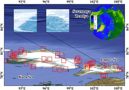
In this study, all samples are located near Severnaya Zemlya (SZ), which is a 37,000 km² archipelago in the Arctic (Figure 7). SZ separates two marginal seas of the Arctic Ocean, the Kara Sea in the west and the Laptev Sea in the east, which are key waters affecting AR navigation. A total of 50 S1 EW scenes, extending from July 2017 to October 2020 (melt seasons), are used in the present study. The nominal pixel spacing of the acquired SAR images is 40 m by 40 m, and the incidence angle ranges from 19° to 47°. We manually select sample data with a size of 1500 × 1500 (60 km × 60 km) from each scene.

Figure 7. Locations of 50 S1 image scenes used for the identification of sea ice and water in the Severnaya Zemlya region.

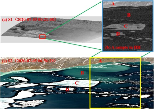
To more efficiently annotate SAR images, both segmentation methods and manual visual interpretation are used. First, the dB ranges for the sea ice and water are calculated from a total of 200 squares of size 10 × 10 using SAR images (HH polarization). We find that sea ice displays backscattering and is brighter in the images than is water in most cases. Therefore, we can establish a classifier, such as through K-means clustering, to preliminarily obtain the boundaries between sea ice and water based on the dB distribution characteristics of samples. Land is not considered in our model, and we apply a land mask to remove land areas using vector boundaries. However, some factors may cause the backscattering characteristics of ice and water to be similar. For example, the pooled melt water on the sea ice surface often reduces the backscattering of the ice surface and makes it darker in images. Additionally, waves make the surface of sea water rougher, thus increasing backscattering. Therefore, these classified samples are converted into vector data using GIS software and further rectified manually by a trained analyst who identifies regions by using overlapping S1 and optical data (Sentinel-2 (S2)). Figure 8 provides an example to show how to distinguish water from sea ice by overlapping S1 and S2 scenes with a difference in acquisition time of less than 8 h and a cloud cover level of < 25%. From the S2 data, we can clearly tell that A denotes land, B denotes ocean, and C and D denote sea ice; however, B, C and D move out of the yellow box because they drift under the influence of wind.

Figure 8. An example of overlapping S1 and S2 for the selection of training data. A denotes land, B denotes ocean, and C and D denote sea ice. Panel (a) shows an S1 scene from 00:21 am July 5, 2020, located in the sea near SZ; (b) shows a selective sample (dB, HH image), and (c) shows an optical S2 scene (red – green – blue (RGB) channels) used to verify the rationality of sample data selection (6: 56 am on July 5, 2020).

To enhance the diversity of samples, we further extract chips from the 50 samples. Each sample is randomly cut into 50 images with a size of 750 × 750. Therefore, there are 2,500 chips available for the training set. Our U-net model is run for 100 training epochs (when the training epochs reach 100, the prediction accuracy and loss of our model reach a stable state). The other parameters are established according to Li’s settings (Li et al. 2020): 80% of the chips are used as training labels and 20% of the chips as test labels to evaluate our model predictions; the convolution operation is performed with 3 × 3 filters for all convolutional layers; downsampling is performed based on a 2 × 2 max pooling operation; the batch size is 16 and the initial learning rate is 0.0001.

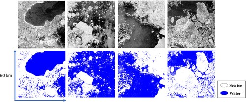
As an example, pixelwise U-Net classifications using 7 selected features for scenes from October 27, 2021, are displayed in Figure 9. Most of the sea ice, including small chunks and sinuous ice edges, can be successfully detected.

Figure 9. The input SAR image (HH) is shown in the upper row, and the inference result is shown in the bottom row. Blue areas represent ocean, and white areas represent sea ice.

3.3. Visualization model

Data visualization (Aparicio and Costa 2015) can be used to transform abstract data into images that are easy to identify and provide users with more intuitive information and knowledge. In this study, Cesium (Aditya et al. 2020; Li and Wang 2017), a WebGL-based virtual globe, is chosen as a 3D GIS platform because it is free to access and commonly used. This virtual globe software program uses satellite imagery, aerial photography, and GISs to perform mapping based on a 3D model of the Earth. Moreover, it is an effective and user-friendly tool for visualizing geospatial data (including images, terrain and calculation results) compared to traditional GIS software. Additionally, GeoServer (Yu et al. 2012), an open-source server for sharing geospatial data, is utilized to publish the calculation results as a Web Map Tile Service (WMTS), which significantly improves the loading speed of the calculation results in Cesium.

3.4. Experiment equipment

RouteView relies on 3 cloud-based virtual machines (VMs) and a 500 TB cloud disk in the BEDCSP. Three VMs are used to realize different functionalities for each model. The No. 1 VM deploys the website program, the No. 2 VM is responsible for computing services, and the No. 3 VM controls data processing and storage. All of the implemented software is open source and includes Cesium, PyTorch, Greenplum, SNAP, File Transfer Protocol (FTP), Python and GDAL functionalities (Qin, Zhan, and Zhu 2014).

4. System application

The RouteView web application (http://arcticroute.tpdc.ac.cn/navigate) was developed with the Cesium framework and the Python programming language; it has two main components: ‘navigation planning’, which guides users through several steps to plan optimal shipping routes along the NEP within 60 days, and ‘sea ice detection’, which provides an interface for real-time sea ice information extraction. These two components provide different levels of decision-making information for Arctic ship route planning from macro – to local scales. In this section, these two components of the currently available version of RouteView are discussed.

4.1. Shipping route planning

Shipping route planning involves a combination of searching for and following the safest and most convenient sailing route from an origin to a destination, which can effectively reduce navigation costs and risks. RouteView provides an online interactive route calculation interface, which can provide optimal navigation planning (daily) for two types of ships (merchant ships and Ice Class PC1 ships that are designed for operation in at least moderate first-year ice) 60 days into the future according to meteorological, sea ice and terrain data.

Figure 10 provides an example of online route calculation. Users can flexibly input the positions of the start and end points of a route, ship types and start time through the 3D GIS interface of RouteView. After submitting these calculation parameters, the system can quickly realize the real-time online extraction of the optimal route under different constraints, and the results are automatically displayed in 3D GIS. The calculation results include the optimal spatial distribution of navigation routes on September 1, 2021, the trip duration, fuel consumption, temporal and spatial changes in sea ice and the risk value along the route, and temperature changes in local sea areas for the coming week. In addition, the first (start) and last (end) dates of NEP transit navigation and the duration of transit navigation are automatically assessed and reported.

Figure 10. The sailing routes of merchant ships on September 1st, 2021 (start and end points can be customized). The data are from the FGOALS-f2 Arctic sea ice prediction system of the Institute of Atmospheric Sciences, Chinese Academy of Sciences.

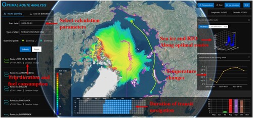
The rapid extraction of this route information provides an important decision-making basis for the navigation of Arctic ships, such as how optimal routes are distributed and when and how long the NEP can be navigable. The whole calculation process is automatically completed in the BEDCSP, and each calculation is performed in less than 3 s.

4.2. Sea ice detection

The sea ice detection model is trained and works well (details are given in Section 3.2.2). We then transfer it to an online platform to reduce complexity in preparing the necessary data and running models. The main purpose of the sea ice detection web application is to provide a user-friendly interface to help end-users quickly access sea ice information at a high resolution.

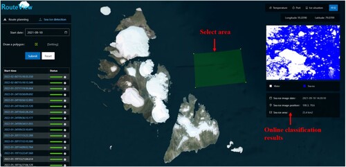
The key functionality of the sea ice detection framework is shown in Figure 11. The user may select the boundary and date to be used as input parameters. After the calculation command is submitted, our system begins the online real-time calculations for sea ice images (the data are for July 15, 2020), and the calculation progress can be viewed through the progress update bar in the left panel. Generally, the calculation time of each scene image (60 km * 60 km) is approximately 3.8 s. After this calculation is completed, the classification results are shown in the right interface, where blue denotes ocean and white represents sea ice. The image date, central latitude and longitude coordinates and sea ice area are also automatically calculated. This information tells users whether there are floes along optimal routes and helps them make reasonable navigation decisions (at a higher resolution than that traditional provided), serving as a further information supplement for the extracted optimal routes.

Figure 11. Online interface for sea ice classification.

5. Validation and evaluation

In this study, we use RL and the deep learning framework U-Net to realize the extraction of the optimal routes and the real-time generation of sea ice images, respectively. In this section, the performance analysis and evaluation process for these two important algorithms used in RouteView are introduced.

5.1. Validation examples for RL

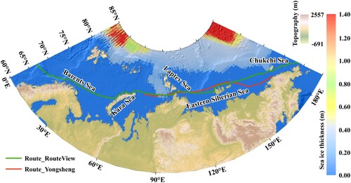
We first analyze the reliability and accuracy of the RL algorithm. Because publicly available sailing routes that can be used by Arctic ships are very limited, we select the Yongsheng merchant shipping route of China COSCO Shipping Corporation Limited as an example (Ma et al. 2019) to verify the effectiveness of our method. The selected ship departed from Dalian Port in China on August 8, 2013, and arrived at Rotterdam Port in the Netherlands after 27 days. As the optimal route calculated in RouteView did not change much during these 27 days (the sea ice and weather conditions near the NEP did not change much during this period), the route calculation result on August 20th is selected for comparison with the actual route traveled by the Yongsheng merchant ship.

In Figure 12, the green route is the optimal route for merchant ships automatically calculated by our system, and the red track is part of the route of the Yongsheng merchant ship. As the actual sailing route is generally extemporaneously decided by the captain according to the ice conditions and meteorological information available at that time, it is influenced by certain subjectivity; thus, the overall trends of the two routes are basically the same, but they do not completely coincident. Moreover, we superimpose the automatically calculated route with the SIT data from the NSIDC, and it is obvious that the proposed route is distributed across areas of low SIT or without sea ice, which significantly improves the safety of ship navigation.

Figure 12. Comparison of two routes. The red line shows the actual sailing route of the Yongsheng ship in September 2013, and the green line shows the optimal route automatically calculated by RouteView. Different colors in the ocean represent different sea ice thicknesses.

Additionally, we compare the advantages and disadvantages of RL and the traditional A* algorithm applied for shipping route planning (Table 3). As shown in Table 3, the traditional A* algorithm displays relatively poor computational efficiency in environments with large grids. Although RL requires model training for the environment, once the model is trained, the prediction speed is very fast, making the model highly suitable for the online calculation of ARs.

Table 3. Advantages and disadvantages of extracting ARs based on the traditional A* algorithm and RL.

Algorithm name	Route extraction time *	Advantages	Disadvantages
A*	29.5 s	There is no need to train the model.	The A* algorithm is computationally intensive when there are too many search nodes in a complex map with many obstacles, so it is difficult to apply in real-time route planning.
RL (DQN)	0.54 s	The prediction speed is very fast. It can extensively explore different states in training and find a more reasonable route.	The model must be trained. In this study, it took approximately 10 min to build the Arctic environmental grid.

* Both RL and the A* algorithm use a standard regular grid (256 rows and 720 columns) to extract routes, and the resolution of the calculation results is 100 km. For RL, 0.54 s is the prediction time.

5.2. Evaluation of the U-Net model

Accurate verification data for Arctic sea ice are difficult to obtain, and most studies use sea ice charts from the Canadian Ice Service (CIS) to verify the classification results of images (Trishchenko and Luo 2021; Tan et al. 2018; Zakhvatkina et al. 2017; Liu, Guo, and Zhang 2015). However, the data area for these charts is limited to Canada's navigable waters. These areas are inconsistent with our research areas. Therefore, in this study, we use 80% of chips as training labels and 20% of chips as test labels to evaluate our model predictions.

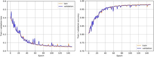
Figure 13 presents the corresponding training and validation loss curves, and as can be observed, both the validation and training losses decrease with increasing number of epochs, reflecting improved generalization capabilities. Our model also displays high and consistent validation accuracy, reaching 0.97.

Figure 13. Losses and accuracy for U-Net model training and validation.

6. Discussion

In this paper, we present RouteView, an intelligent online system for route planning. This new system offers an easy-to-use graphical user interface (GUI) to calculate optimal routes and extract sea ice information in real time. In the following subsections, we discuss the performance and advantages of this system as well as the associated challenges and limitations.

6.1. System performance and advantages

Although there are many studies that performed route analysis, these studies focus on route planning algorithms or optimization models (Zvyagina and Zvyagin 2022), which were static, and cannot be directly used to guide shipping navigation in the variable, harsh environment of the Arctic. Recent years, some systems for route optimization in ice-covered waters were developed, however, the automated workflow and calculation efficiency for these systems (Kotovirta et al. 2009; Mannarini et al. 2013, 2019; Vettor and Guedes Soares 2016) still need to be improved. In this study, an online interactive computing framework is developed, and two online computing cases involving route calculation and sea ice classification are explored. Overall, with the proposed approach, the computational procedure is simplified in three respects.

First, our new system can automatically download and process data according to the relevant computing requirements. Due to the use of cache technology, downloaded data or processed intermediate results can be quickly used by other related calculation processes. For users, all data can be easily accessed without requiring detailed complex processing steps in the downloading and preprocessing stages.

Second, the newly developed system can greatly improve the efficiency of analysis. Users simply need to input or calculate some parameters, and all other steps are performed automatically by the system, which greatly reduces the cost and difficulty of route planning for researchers. Additionally, the computational time is reduced by combining algorithms, distributed computing resources and other big data technologies, such as MPP databases (Wu, Guo, and Yang 2020), graphics processing units (GPUs) and distributed computing strategies. We counted the average response time of each functional module, and the average usage time was no more than 4 s, as shown in Table 4.

Table 4. Average response times of submodule functions.

No.	Functional module	Response time (unit: second)
1	Calculating the optimal route distributions	0.54
2	Calculating the changes in ice conditions and navigation risks along optimal routes	1.8
3	Calculating the temperature changes in the concerned areas in the coming week	2.1
4	Calculating the sea ice distribution (60 km * 60 km)	3.8

Third, we deconstructed the full process of information extraction processing into three relatively separate modules, including data, calculation and visualization modules. Each module is encapsulated by a web service (Hamid et al. 2019), which reduces coupling between modules and increases the flexibility of the function of each module. For example, we can flexibly replace analytical methods and available data without affecting the operation of the system.

6.2. Challenges and limitations

Despite its several advances, RouteView also has certain limitations. In terms of sea ice information extraction, we use SAR data to quickly extract accurate and reliable sea ice images. Although the revisit time in the Arctic for the data is less than one day, these single-source data do not allow for further improvements in the accuracy of remote sensing sea ice classification. To improve classification accuracy, heterogeneous data fusion tools, such as those based on SAR data and optical remote sensing images, should be applied in the classification of sea ice in future work (Han et al. 2021). Moreover, the deep learning framework based on U-Net can classify sea water and sea ice at the pixel level, but do not further classify types of sea ice. For example, sea ice can be further divided into young ice, first-year sea ice, and multiyear sea ice (Aldenhoff, Heuzé, and Eriksson 2019). Additionally, our goal was to provide a full account of online computing workflows but not to develop an innovative sea ice classification method. Hence, only a verification analysis of accuracy is provided in the U-Net sea ice classification method, and a comparison with other deep learning framework methods remains an open issue. Therefore, we plan to perform more testing and comparisons of different algorithms in future work. Last, due to the limitations of server storage, we cannot download all S1 data to a server; we can only download the required data in real time or completely download data for key sea areas in advance according to the user's need to quickly extract information. Therefore, we only select SZ as a research area to test the effectiveness of the system calculation processes. Due to these limitations, we do not use the ice-water classification results calculated by our system as the input for the optimal route calculation and instead use publicly released sea ice products to analyze the route distribution.

7. Conclusion and future work

Processing massive spatiotemporal data and automatically extracting information for Arctic navigation tasks over time have become urgent problems in the era of big data. In this article, we developed an online interactive route planning system (RouteView) for ships sailing in the Arctic. The process of transforming raw data into analysis results is fully automated with this approach (facilitating the transition from big data to valuable information). This new system improves the intelligence level of AR information services from two perspectives: (1) optimal routes are automatically explored without human intervention, and (2) high-resolution ice information in local sea areas can be automatically extracted.

The experimental results show that RouteView can greatly reduce the barriers users experience in planning optimal routes and efficiently extracting sea ice information. The optimal route distribution along the NEP can be calculated 60 days into the future under different conditions within 1 s, and the ice-water classification results can be obtained within 3 s for images in the range of 60 km × 60 km. This newly developed system is easy to use, freely available and an open source tool. More importantly, the online computing framework used by this system can be applied not only for route analysis and decision-making in the Arctic but also for reference and utilization in related geoscience fields.

In future work, we will try to solve the problems mentioned in the previous section by expanding the sea ice dataset and adjusting the model network structure. In addition, our system will focus on addressing the following questions: with the implementation of World's goals of ‘carbon peak and carbon neutralization’, how will the change in World's energy demand affect the utility of the Arctic route in the future; how will the navigation cost of ordinary merchant ships traveling along ARs change with the further melting of Arctic sea ice in the summer; and how should shipping companies choose ARs, conventional southern routes (e.g. the Suez Canal) and Railway Express routes?

System availability

The information for the main software modules used in RouteView is as follows: Operating system version: CentOS7.5 (Linux version 3.10.0862.14.4.el7.x86_64)

Greenplum version: GP Database 6.0.0alpha.0Cdev.7321.gb7ce9c4

Python version: 3.6

SNAP version: 8.0

PyTorch version: 1.7.1

GDAL version: 2.2.3

Acknowledgments

Since model implementation in 2020, the construction of RouteView has been aided by Professors Anmin Duan and Bian He from the Institute of Atmospheric Physics, Chinese Academy of Sciences. We would like to express sincere appreciation to them for their work related to sea ice data services. The CAS Big Earth Data Science Engineering (CASEarth) program provides a system operation environment. We are also grateful to the editor and the anonymous reviewers for their valuable comments and suggestions, which have improved the presentation of the manuscript.

Data availability statement

Data are openly available in a public repository that does not issue DOIs. The sea ice thickness, sea ice conditions and wind speed used for route analysis in our system are publicly available at http://project.lasg.ac.cn/FGOALS_f2-S2S/index.php?Var = Arctic-sea-ice. In addition, model bathymetry is publicly available at https://www.ngdc.noaa.gov/mgg/global/relief/ETOPO1/data/bedrock/grid_registered, and Sentinel-1 data can be downloaded at https://scihub.copernicus.eu/dhus/#/home.

Disclosure statement

No potential conflict of interest was reported by the author(s).

Additional information

Funding

This work was supported by the Strategic Priority Research Program of the Chinese Academy of Science under (Grant no XDA19070101).

References

- Aase, Johnny Grøneng, and Julia Jabour. 2015. “Can Monitoring Maritime Activities in the European High Arctic by Satellite-Based Automatic Identification System Enhance Polar Search and Rescue?” The Polar Journal 5 (2): 386–402.
- Aditya, Trias, Dany Laksono, Febrian F. Susanta, I. Istarno, D. Diyono, and Didik Ariyanto. 2020. “Visualization of 3D Survey Data for Strata Titles.” ISPRS International Journal of Geo-Information 9 (5): 310–330.
- Ahmed, Zeinab E, Rashid A Saeed, Amitava Mukherjee, and Sheetal N Ghorpade. 2020. Energy optimization in low-power wide area networks by using heuristic techniques.” LPWAN Technologies for IoT and M2M Applications:199-223.
- Aldenhoff, Wiebke, Céline Heuzé, and Leif E. Eriksson. 2019. “Sensitivity of Radar Altimeter Waveform to Changes in Sea Ice Type at Resolution of Synthetic Aperture Radar.” Remote Sensing 11 (22): 2602.
- Aparicio, Manuela, and Carlos J. Costa. 2015. “Data Visualization.” Communication Design Quarterly 3 (1): 7–11.
- Bharati, Manish H., Jay J. Liu, and John F. MacGregor. 2004. “Image Texture Analysis: Methods and Comparisons.” Chemometrics and Intelligent Laboratory Systems 72 (1): 57–71.
- Blackport, Russell, and James A. Screen. 2020. “Insignificant Effect of Arctic Amplification on the Amplitude of Midlatitude Atmospheric Waves.” Science Advances 6 (8): eaay2880.
- Buixadé Farré, Albert, Scott R Stephenson, Linling Chen, Michael Czub, Ying Dai, Denis Demchev, Yaroslav Efimov, Piotr Graczyk, Henrik Grythe, and Kathrin Keil. 2014. “Commercial Arctic Shipping Through the Northeast Passage: Routes, Resources, Governance, Technology, and Infrastructure.” Polar Geography 37 (4): 298–324.
- Chang, K. Y., S. S. He, C. C. Chou, S. L. Kao, and A. S. Chiou. 2015. “Route Planning and Cost Analysis for Travelling Through the Arctic Northeast Passage Using Public 3D GIS.” International Journal of Geographical Information Science 29 (8): 1375–1393.
- Chen, Shiyi, Yunfeng Cao, Fengming Hui, and Xiao Cheng. 2019. “Observed Spatial-Temporal Changes in the Autumn Navigability of the Arctic Northeast Route from 2010 to 2017.” Chinese Science Bulletin 64 (14): 1515–1525.
- Chen, Jinlei, Shichang Kang, Wentao Du, Junming Guo, Min Xu, Yulan Zhang, Xinyue Zhong, Wei Zhang, and Jizu Chen. 2021. “Perspectives on Future sea ice and Navigability in the Arctic.” The Cryosphere 15 (12): 5473–5482.
- Chen, Shiyi, Mohammed Shokr, Xinqing Li, Yufang Ye, Zhilun Zhang, Fengming Hui, and Xiao Cheng. 2020. “MYI Floes Identification Based on the Texture and Shape Feature from Dual-Polarized Sentinel-1 Imagery.” Remote Sensing 12 (19): 1–22.
- Christodoulou, Anastasia, Dimitrios Dalaklis, Peter Raneri, and Rebecca Sheehan. 2022. “An Overview of the Legal Search and Rescue Framework and Related Infrastructure Along the Arctic Northeast Passage.” Marine Policy 138: 104985.
- Cohen, Judah, Karl Pfeiffer, and Jennifer A. Francis. 2018. “Structural Absorption by Barbule Microstructures of Super Black Bird of Paradise Feathers.” Nature Communications 9 (1): 1–12.
- Dai, Aiguo, Dehai Luo, Mirong Song, and Jiping Liu. 2019. “Double-slit Photoelectron Interference in Strong-Field Ionization of the Neon Dimer.” Nature Communications 10 (1): 1–13.
- David, Malmgren H., Leif T. Pedersen, Allan A. Nielsen, Matilde B. Kreiner, and Klaus H. Krane. 2021. “A Convolutional Neural Network Architecture for Sentinel-1 and AMSR2 Data Fusion.” IEEE Transactions on Geoscience and Remote Sensing 59 (3): 1890–1902.
- Delgado Blasco, José Manuel, Michael Foumelis, Chris Stewart, and Andrew Hooper. 2019. “Measuring Urban Subsidence in the Rome Metropolitan Area (Italy) with Sentinel-1 SNAP-StaMPS Persistent Scatterer Interferometry.” Remote Sensing 11 (2): 1–17.
- Dijkstra, E. W. 1959. “A Note on Two Problems in Connexion with Graphs.” Numerische Mathematik 1: 269–271.
- Dong, Liangxiong, Jun Li, Wei Xia, and Qiang Yuan. 2021. “Double ant Colony Algorithm Based on Dynamic Feedback for Energy-Saving Route Planning for Ships.” Soft Computing 25 (7): 5021–5035.
- Dorigo, Marco, Mauro Birattari, and Thomas Stutzle. 2006. “Ant Colony Optimization.” IEEE Computational Intelligence Magazine 1 (4): 28–39.
- Fang, Miao, Xin Li, W. Hans Chen, and Deliang Chen. 2022. “Arctic Amplification Modulated by Atlantic Multidecadal Oscillation and Greenhouse Forcing on Multidecadal to Century Scales.” Nature Communications 13, doi:10.1038/s41467-022-29523-x.
- Gao, Yunhao, Feng Gao, Junyu Dong, and Shengke Wang. 2019. “Transferred Deep Learning for sea ice Change Detection from Synthetic-Aperture Radar Images.” IEEE Geoscience and Remote Sensing Letters 16 (10): 1655–1659.
- Gu, Wei, Zhihan Lv, and Ming Hao. 2017. “Change Detection Method for Remote Sensing Images Based on an Improved Markov Random Field.” Multimedia Tools and Applications 76 (17): 17719–17734.
- Gunnarsson, Bjørn. 2013. “Knowledge Transfer and Cooperation on Shipping and Logistics in the High North.” Futures of Northern Cross-Border Collaboration: 61–76.
- Hamid, Sawsan A., Rana A. Abdalrahman, Inam A. Lafta, and Israa A. Barazanchi. 2019. “Distance and Travel Time Modeling in High-Level Picker-To-Part Systems (3-D Warehouses).” Journal of Southwest Jiaotong University 54 (6): 1–10.
- Han, Yanling, Yekun Liu, Zhonghua Hong, Yun Zhang, Shuhu Yang, and Jing Wang. 2021. “Sea Ice Image Classification Based on Heterogeneous Data Fusion and Deep Learning.” Remote Sensing 13 (4): 592–605.
- Hart, P. E., N. J. Nilsson, and B. Raphael. 1972. “A Formal Basis for the Heuristic Determination of Minimum Cost Paths.” IEEE Transactions on Systems Science & Cybernetics 4 (2): 28–29.
- Haydari, Ammar, and Yasin Yilmaz. 2020. “Deep Reinforcement Learning for Intelligent Transportation Systems: A Survey.” IEEE Transactions on Intelligent Transportation Systems 31: 585–589.
- Hinton, Geoffrey E., and Ruslan R. Salakhutdinov. 2006. “Reducing the Dimensionality of Data with Neural Networks.” Science 313 (5786): 504–507.
- Jegou, Herve, Matthijs Douze, and Cordelia Schmid. 2011. “Product Quantization for Nearest Neighbor Search.” IEEE Transactions on Pattern Analysis and Machine Intelligence 33 (1): 117–128.
- Kang, Tian, Shaodian Zhang, Youlan Tang, Gregory W. Hruby, Alexander Rusanov, Noémie Elhadad, and Chunhua Weng. 2017. “EliIE: An Open-Source Information Extraction System for Clinical Trial Eligibility Criteria.” Journal of the American Medical Informatics Association 24 (6): 1062–1071.
- Khaleghian, Salman, Habib Ullah, Thomas Kræmer, Nick Hughes, Torbjørn Eltoft, and Andrea Marinoni. 2021. “Sea ice Classification of SAR Imagery Based on Convolution Neural Networks.” Remote Sensing 13 (9): 1–20.
- Kotovirta, V., R. Jalonen, L. Axell, K. Riska, and R. Berglund. 2009. “A System for Route Optimization in ice-Covered Waters.” Cold Regions Science and Technology 55 (1): 52–62.
- Lample, Guillaume, and Devendra S. Chaplot. 2017. Playing FPS games with deep reinforcement learning.” In Thirty-First AAAI Conference on Artificial Intelligence.
- Li, Jinxiao, Qing Bao, Yimin Liu, Guoxiong Wu, Lei Wang, Bian He, Xiaocong Wang, Jing Yang, Xiaofei Wu, and Zili Shen. 2021. “Dynamical Seasonal Prediction of Tropical Cyclone Activity Using the FGOALS-f2 Ensemble Prediction System.” Weather and Forecasting 36 (5): 1759–1778.
- Li, Xin, Tao Che, Xinwu Li, Lei Wang, Anmin Duan, Donghui Shangguan, Xiaoduo Pan, Miao Fang, and Qing Bao. 2020. “CASEarth Poles: Big Data for the Three Poles.” Bulletin of the American Meteorological Society 101 (9): E1475–E1491.
- Li, Xin, Guodong Cheng, Liangxu Wang, Juanle Wang, Youhua Ran, Tao Che, Guoqing Li, Honglin He, Qiang Zhang, and Xiaoyi Jiang. 2021. “Boosting Geoscience Data Sharing in China.” Nature Geoscience 14 (8): 541–542.
- Li, Jiayi, Xin Huang, and Jianya Gong. 2019. “Deep Neural Network for Remote-Sensing Image Interpretation: Status and Perspectives.” National Science Review 6 (6): 1082–1086.
- Li, Xiaofeng, Bin Liu, Gang Zheng, Yibin Ren, Shuangshang Zhang, Le Gao Yingjie Liu, Yuhai Liu, Bin Zhang, and Fan Wang. 2020. “Deep-learning-based Information Mining from Ocean Remote-Sensing Imagery.” National Science Review 7 (10): 1584–1605.
- Li, Wenwen, and Sizhe Wang. 2017. “PolarGlobe: A web-Wide Virtual Globe System for Visualizing Multidimensional, Time-Varying, big Climate Data.” International Journal of Geographical Information Science 31 (8): 1562–1582.
- Li, Songnian, Chenfeng Xiong, and Ziqiang Ou. 2011. “A Web GIS for sea ice Information and an ice Service Archive.” Transactions in GIS 15 (2): 189–211.
- Liu, Huiying, Huadong Guo, and Lu Zhang. 2015. “SVM-Based Sea Ice Classification Using Textural Features and Concentration from RADARSAT-2 Dual-Pol ScanSAR Data.” IEEE Journal of Selected Topics in Applied Earth Observations and Remote Sensing 8 (4): 1601–1613.
- Lohse, Johannes, Anthony P. Doulgeris, and Wolfgang Dierking. 2021. “Incident Angle Dependence of Sentinel-1 Texture Features for Sea Ice Classification.” Remote Sensing 13 (4): 1–19.
- Long, Jonathan, Evan Shelhamer, and Trevor Darrell. 2015. “Fully Convolutional Networks for Semantic Segmentation.” IEEE Transactions on Pattern Analysis and Machine Intelligence 39 (4): 640–651.
- Lyu, Hangyu, Weimin Huang, and Masoud Mahdianpari. 2022. “A Meta-Analysis of Sea Ice Monitoring Using Spaceborne Polarimetric SAR: Advances in the Last Decade.” IEEE Journal of Selected Topics in Applied Earth Observations and Remote Sensing 15: 6158–6179.
- Ma, Long, Lei An, Xiaohui Zhang, Zhongyi Zheng, Zhenghua Li, and Guanwen Chen. 2019. “Navigable Window Dataset of the Arctic Northeast Passage (2006–2015).” Journal of Global Change Data & Discovery 3 (3): 244–250.
- Mäkynen, Marko, Stefan Kern, Anja Rösel, and Leif Toudal Pedersen. 2014. “On the Estimation of Melt Pond Fraction on the Arctic Sea ice with ENVISAT WSM Images.” IEEE Transactions on Geoscience and Remote Sensing 52 (11): 7366–7379.
- Mannarini, G., G. Coppini, P. Oddo, and N. Pinardi. 2013. “A Prototype of Ship Routing Decision Support System for an Operational Oceanographic Service.” TransNav: International Journal on Marine Navigation and Safety of Sea Transportation 7 (1): 53–59.
- Mannarini, G., G. Coppini, P. Oddo, and N. Pinardi. 2019. “Preliminary Inter-Comparison of AIS Data and Optimal Ship Tracks.” TransNav, the International Journal on Marine Navigation and Safety of Sea Transportation 13 (1).
- Mikołajczyk, Agnieszka, and Michał Grochowski. 2018. Data augmentation for improving deep learning in image classification problem.” Paper presented at the 2018 international interdisciplinary PhD workshop (IIPhDW), Świnoujście.
- Minaee, Shervin, Yuri Y. Boykov, Fatih Porikli, Antonio J. Plaza, Nasser Kehtarnavaz, and Demetri Terzopoulos. 2021. “Image Segmentation Using Deep Learning: A Survey.” IEEE Transactions on Pattern Analysis and Machine Intelligence 1: 1–1.
- Mirończuk, Marcin Michał. 2018. “The BigGrams: The Semi-Supervised Information Extraction System from HTML: An Improvement in the Wrapper Induction.” Knowledge and Information Systems 54 (3): 711–776.
- Mnih, Volodymyr, Koray Kavukcuoglu, David Silver, Andrei A Rusu, Joel Veness, Marc G Bellemare, Alex Graves, Martin Riedmiller, Andreas K Fidjeland, and Georg Ostrovski. 2015. “Human-level Control Through Deep Reinforcement Learning.” Nature 518 (7540): 529–533.
- Mulherin, Nathan D., Devinder S. Sodhi, and Duane T. Eppler. 1999. NSRSIM2A: a time and cost prediction model for Northern Sea Route Shipping, Paper presented at International Northern Sea Route Programme (INSROP), March.
- Nam, Jong H., Inha Park, Ho J. Lee, Mi O. Kwon, Kyungsik Choi, and Young K. Seo. 2013. “Simulation of Optimal Arctic Routes Using a Numerical sea ice Model Based on an ice-Coupled Ocean Circulation Method.” International Journal of Naval Architecture and Ocean Engineering 5 (2): 210–226.
- Numbisi, Frederick N., Frieke V. Coillie, and Robert D. Wulf. 2019. “Delineation of Cocoa Agroforests Using Multiseason Sentinel-1 SAR Images: A low Grey Level Range Reduces Uncertainties in GLCM Texture-Based Mapping.” ISPRS International Journal of Geo-Information 8 (4): 1–25.
- Öztürk, Şaban, and Bayram Akdemir. 2018. “Application of Feature Extraction and Classification Methods for Histopathological Image Using GLCM, LBP, LBGLCM, GLRLM and SFTA.” Procedia Computer Science 132: 40–46.
- Pan, Xiaoduo, Xuejun Guo, Xin Li, Xiaolei Niu, Xiaojuan Yang, Min Feng, Tao Che, Rui Jin, Youhua Ran, and Jianwen Guo. 2021. “National Tibetan Plateau Data Center: Promoting Earth System Science on the Third Pole.” Bulletin of the American Meteorological Society 102 (11): E2062–E2078.
- Qin, Chengzhi, Lijun Zhan, and Axing Zhu. 2014. “How to Apply the Geospatial Data Abstraction Library (GDAL) Properly to Parallel Geospatial Raster I/O?” Transactions in GIS 18 (6): 950–957.
- Radhakrishnan, Keerthijan, Andrea Scott, and David Clausi. 2021. “Sea Ice Concentration Estimation: Using Passive Microwave and SAR Data with a U-net and Curriculum Learning.” IEEE Journal of Selected Topics in Applied Earth Observations and Remote Sensing PP 99: 1–1.
- Reichstein, Markus, Gustau Camps-Valls, Bjorn Stevens, Martin Jung, Joachim Denzler, and Nuno Carvalhais. 2019. “Deep Learning and Process Understanding for Data-Driven Earth System Science.” Nature 566 (7743): 195–204.
- Ren, Yibin, Xiaofeng Li, Xiaofeng Yang, and Huan Xu. 2021. “Development of a Dual-Attention U-Net Model for Sea Ice and Open Water Classification on SAR Images.” IEEE Geoscience and Remote Sensing Letters. doi:10.1109/TGRS.2022.3177600.
- Ronneberger, Olaf, Philipp Fischer, and Thomas Brox. 2015. U-net: Convolutional networks for biomedical image segmentation.” Paper presented at the International Conference on Medical image computing and computer-assisted intervention.
- Şahin, Bekir. 2019. “Route Prioritization by Using Fuzzy Analytic Hierarchy Process Extended Dijkstra Algorithm.” Journal of ETA Maritime Science 7 (1): 3–15.
- Sallab, Ahmad EL, Mohammed Abdou, Etienne Perot, and Senthil Yogamani. 2017. “Deep Reinforcement Learning Framework for Autonomous Driving.” Electronic Imaging 29 (19): 70–76.
- Shyu, Wen-Hwa, and Ji-Feng Ding. 2016. “Key Factors Influencing the Building of Arctic Shipping Routes.” Journal of Navigation 69 (6): 1261–1277.
- Silver, David, Aja Huang, Chris J. Maddison, Arthur Guez, Laurent Sifre, George V. D. Driessche, and Julian Schrittwieser. 2017. “Mastering the Game of Go without Human Knowledge.” Nature 550 (7676): 354–359.
- Stoddard, M. A., L. Etienne, M. Fournier, R. Pelot, and L. Beveridge. 2017. “Making Sense of Arctic Maritime Traffic Using the Polar Operational Limits Assessment Risk Indexing System (POLARIS).” IOP Conference Series: Earth and Environmental Ence 34 (1): 012034.
- Tan, Weikai, Jonathan Li, Linlin Xu, and Michael A. Chapman. 2018. “Semiautomated Segmentation of Sentinel-1 SAR Imagery for Mapping sea ice in Labrador Coast.” IEEE Journal of Selected Topics in Applied Earth Observations and Remote Sensing 11 (5): 1419–1432.
- Tang, Xueying, Yunxiao Chen, Xiaoou Li, Jingchen Liu, and Zhiliang Ying. 2019. “A Reinforcement Learning Approach to Personalized Learning Recommendation Systems.” British Journal of Mathematical and Statistical Psychology 72 (1): 108–135.
- Thoman, Richard L., Jacqueline Richter-Menge, and Matthew L. Druckenmiller. 2020. “NOAA Arctic Report Card 2020 Executive Summary.” doi:10.25923/mn5p-t549.
- Trishchenko, Alexander P, and Yi Luo. 2021. “Landfast Ice Mapping Using MODIS Clear-Sky Composites: Application for the Banks Island Coastline in Beaufort Sea and Comparison with Canadian Ice Service Data.” Canadian Journal of Remote Sensing 47 (1): 143–158.
- Tsou, Ming C., and Hung C. Cheng. 2013. “An Ant Colony Algorithm for Efficient Ship Routing.” Polish Maritime Research 20 (3): 28–38. doi:10.2478/pomr-2013-0032.
- Vettor, Roberto, and C. Guedes Soares. 2016. “Development of a Ship Weather Routing System.” Ocean Engineering 123: 1–14.
- Volodymyr, Mnih, Kavukcuoglu Koray, Silver David, Andrei A. Rusu, Veness Joel, Marc G. Bellemare, Graves Alex, Riedmiller Martin, Andreas K. Fidjeland, and Ostrovski Georg. 2015. “Human-level Control Through Deep Reinforcement Learning.” Nature 518 (7540): 529–533.
- Wang, Lei, K. Andrea Scott, and David A. Clausi. 2017. “Sea ice Concentration Estimation During Freeze-up from SAR Imagery Using a Convolutional Neural Network.” Remote Sensing 9 (5): 1–10.
- Wang, Yanjun, Fuchao Li, Bin Zhang, and Xiaofeng Li. 2022. “Development of a Component-Based Interactive Visualization System for the Analysis of Ocean Data.” Big Earth Data 6 (2): 219–235.
- Wang, Yangjun, Ren Zhang, and Longxia Qian. 2018. “An Improved A* Algorithm Based on Hesitant Fuzzy Set Theory for Multi-Criteria Arctic Route Planning.” Symmetry 10 (12): 1–10.
- Wang, Shupeng, Weigang Zhao, Guangyuan Zhang, Hongbin Xu, and Yanliang Du. 2021. “Identification of Structural Parameters from Free Vibration Data Using Gabor Wavelet Transform.” Mechanical Systems and Signal Processing 147: 1–10.
- Wu, Adan, Tao Che, Xin Li, and Xiaowen Zhu. 2022. “A Ship Navigation Information Service System for the Arctic Northeast Passage Using 3D GIS Based on big Earth Data.” Big Earth Data: 1–27. doi:10.1080/20964471.2021.1981197.
- Wu, Adan, Jianwen Guo, and Pengfei Yang. 2020. “Research on Data Sharing Architecture for Ecological Monitoring Using Iot Streaming Data.” IEEE Access 8: 195385–195397.
- Xu, Yan, and K. Andrea Scott. 2017. Sea ice and open water classification of sar imagery using cnn-based transfer learning.” Paper presented at the 2017 IEEE International Geoscience and Remote Sensing Symposium (IGARSS), Fort Worth, United States, July 23 - 28.
- Xu, Hua, and Dong Yang. 2020. “LNG-fuelled Container Ship Sailing on the Arctic Sea: Economic and Emission Assessment.” Transportation Research Part D: Transport and Environment 87: 1–12.
- Yu, Xinwen, Hongyu Liu, Yanchen Yang, Xu Zhang, and Yingwu Li. 2012. GeoServer based forestry spatial data sharing and integration.” Paper presented at the International Conference on Sustainable Energy and Environmental Engineering (ICSEEE 2012), Guangzhou, China, December 29–30.
- Yumashev, Dmitry, Karel V. Hussen, Johan Gille, and Gail Whiteman. 2017. “Towards a Balanced View of Arctic Shipping: Estimating Economic Impacts of Emissions from Increased Traffic on the Northern Sea Route.” Climatic Change 143 (1): 143–155.
- Zakhvatkina, Natalia, Anton Korosov, Stefan Muckenhuber, Stein Sandven, and Mohamed Babiker. 2017. “Operational Algorithm for ice–Water Classification on Dual-Polarized RADARSAT-2 Images.” The Cryosphere 11 (1): 33–46.
- Zhang, Bin, Fuchao Li, Gang Zheng, Yanjun Wang, Zhetao Tan, and Xiaofeng Li. 2021. “Developing big Ocean System in Support of Sustainable Development Goals: Challenges and Countermeasures.” Big Earth Data 5 (4): 557–575.
- Zhang, Minyang, Di Zhang, Shanshan Fu, Xinping Yan, and Chi Zhang. 2017. A method for planning Arctic sea routes under multi-constraint conditions.” Paper presented at the The 24th International Conference on Port and Ocean Engineering under Arctic Conditions, Busan, South Korea, June 11–17.
- Zhang, Chi, Di Zhang, Mingyang Zhang, and WenGang Mao. 2019. “Data-Driven Ship Energy Efficiency Analysis and Optimization Model for Route Planning in Ice-Covered Arctic Waters.” Ocean Engineering 186: 1–10.
- Zhao, Jiechen, Jingjing Cheng, Zhongxiang Tian, Xiaopeng Han, Hui Shen, Guanghua Hao, Honglin Guo, and Qi Shu. 2022. “Snow and Ice Thicknesses Derived from Fast Ice Prediction System Version 2.0 (FIPS V2. 0) in Prydz Bay, East Antarctica: Comparison with in-Situ Observations.” Big Earth Data: 1–12. doi:10.1080/20964471.2021.1965371.
- Zhu, Xinni, Wenzhang Cao, and Wanzheng Ai. 2018. “The Study on Necessity of Actively Participating in Opening up the Arctic Northeast Passage.” IOP Conference Series: Earth and Environmental Science 189 (6): 062042.
- Zvyagin, Petr, and Anna Voitkunskaia. 2016. Model of transit transport in arctic based on graph algorithms.” Paper presented at the Asme International Conference on Ocean, Trondheim, Norway, June 18–21.
- Zvyagina, T., and P. Zvyagin. 2022. “A Model of Multi-Objective Route Optimization for a Vessel in Drifting ice.” Reliability Engineering & System Safety 218: 108147.