Construction of rhombic triacontahedron discrete global grid systems

ABSTRACT

Discrete Global Grid System (DGGS) is a new multi-resolution geospatial data modeling and processing scheme for the digital earth. The icosahedron is commonly regarded as an ideal polyhedron for constructing DGGSs with small distortions; however, the shape of its face is triangular, making it difficult to incorporate the matrix structure used for geospatial data storage and parallel computing. To overcome this limitation, this study utilizes the rhombic triacontahedron (RT) as the basic polyhedron to construct DGGSs. An equal-area projection between the surface of RT and the sphere is developed and used to design a grid-generation algorithm for the aperture 4 hexagonal DGGS based on RT. Compared with the equal-area DGGS based on the icosahedron, the proposed scheme results in smaller angular projection distortions, with the mean and standard deviation decreasing by 41.6% and 30.9%, respectively. The grid cells of the RT DGGS also achieve more optimized geometric characteristics in shape compactness, length deviation, and angle deviation than those in the icosahedron DGGS. Additionally, the cross-surface computation efficiency provides advantages in code conversion to latitude and longitude and proximity queries. Furthermore, the use of RT offers a new and better framework within the context of DGGS research and application.

KEYWORDS:

• Discrete global grid system
• rhombic triacontahedron
• equal-area projection
• hexagon

1. Introduction

Geospatial data acquisition technology has developed rapidly in the wake of the twenty-first century. Large-scale (including global) multi-resolution and multi-type geospatial data are increasingly and frequently used in urban planning, economic development, emergency response to hazards, land and resource management, infrastructure and facilities management, and global environmental change monitoring among other applications for high-quality decision-making (Tang et al. 2021; Peterson 2016; Zhao et al. 2016; Goodchild et al. 2012). However, the organization, management, analysis, and application of vast earth observation data pose severe challenges for academia and the industry (Yao et al. 2019).

The Discrete Global Grid System (DGGS) is a novel geospatial data modeling and processing scheme that partitions the earth using specific methods to form a seamless multi-resolution grid hierarchical structure (Thompson et al. 2022; Bowater and Stefanakis 2019; Sahr, White, and Kimerling 2003). Compared with the traditional spatial data organization and application model based on local projection, DGGS is more suitable for solving large-scale problems and supports the efficient processing of multi-resolution data within the structure.

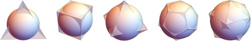
Various DGGSs have been designed to meet specific needs (Hojati et al. 2022; Han et al. 2021; Rawson, Sabeur, and Brito 2021; Qu et al. 2020), but the broadest development prospect is the class based on the polyhedron (Sahr, White, and Kimerling 2003). The more faces a platonic solid has, the smaller is the angle distortion when the grid of the polyhedral surface is mapped to the sphere. The icosahedron has the highest number of faces among five platonic solids (Figure 1). Therefore, the icosahedron is generally considered by the academic community to be the most effective method for obtaining a DGGS with uniform cell geometry.

Figure 1. Platonic solids and their equal-area sphere: the tetrahedron, cube, octahedron, dodecahedron, and icosahedron.

Many scholars have studied the icosahedral DGGS in-depth. Sahr (2008) designed the Icosahedral Snyder Equal-Area Aperture 3 Hexagon DGGS (ISEA3H) and studied the coding index scheme of the grid system. Peterson (2011) proposed the PYXIS coding index scheme based on the ISEA3H and developed the spatial data processing software, WorldView. The Soil Moisture and Ocean Salinity (SMOS) satellite was launched by the European Space Agency (ESA) in 2009 using the Icosahedral Snyder Equal-area Aperture 4 Hexagon DGGS (ISEA4H) to collect and process soil moisture and ocean salinity data (Suess et al. 2004). Ben et al. (2018) developed and improved the hexagonal DGGS generation algorithm. Zhou et al. (2020a) further optimized the location scheme of the icosahedron and extended it to an arbitrary platonic solid. Wang et al. (2020, 2021) and Zhou et al. (2020b) improved the hexagonal icosahedral DGGS coding mathematical model with the help of complex numbers.

Thus, extensive research has been conducted on the icosahedral DGGS in academia. However, this approach has significant limitations. Specifically, the icosahedron DGGS has the drawback of being very different from the spherical shape of the earth and polyhedral surfaces and having a nonuniform grid cell distribution. This results in low precision outputs, which largely stem from inaccurate earth fitting. In addition, the single face of the icosahedron is triangular, which is incompatible with the commonly used rectangle for data organization and storage, thus complicating the arithmetic and reducing the data processing efficiency. This necessitates the innovation and construction of a more practicable DGGS to address the aforementioned limitations (Sahr, White, and Kimerling 2003).

This study proposes the use of a new ideal polyhedron to build DGGSs that combines existing platonic solid modeling methods. In the Catalan polyhedron family (Weisstein 2022a), the rhombic triacontahedron (RT) comprises 30 rhombuses, which are congruent and spatially symmetric (Figure 2). The cell indexing algorithm is simplified by its structure. An RT is closer to a sphere than an icosahedron. Although the use of coordinate-based code may be convenient for indexing or matrix storage on the rhombus surface, the use of the row and column numbers for indexing or matrix storage may be more convenient. Using the triangular surface to construct the rhombus and then perform the unit coding indexing is unnecessary, unlike platonic solids. The recursive division of the icosahedron surface can generate the same equal-area cells, which is suitable for building equal-area grids.

In the standard subdivision graphics for building a DGGS, the hexagon has consistent connectivity and the highest sampling efficiency. Its sphere may present additional advantages, which would be beneficial for geospatial data processing and extensive application (Kimerling et al. 1999; Sahr, White, and Kimerling 2003). Therefore, this study adopts the RT as the initial polyhedron and the hexagon as the grid cell, examines the relationship between the RT surface and the spherical surface, and designs a multi-resolution grid-generation algorithm to establish a new DGGS method. The advantages of this method are demonstrated by experiments that compare it with traditional methods that apply the icosahedron.

2. Basic idea

In the hexagonal grid system, the directions of the cells at different levels of the aperture 4 hexagonal grid system are fixed. They can be associated with quadtree coding and binary operations, which contribute to the efficient operation of the computer. The RT hexagonal DGGS proposed in this study (Figure 3) is constructed by integrating the characteristics of the aperture 4 hexagonal division.

Figure 2. Rhombic triacontahedron (RT) (a) and its corresponding spherical RT (b).

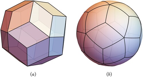
Figure 3. Construction process of the RT DGGS.

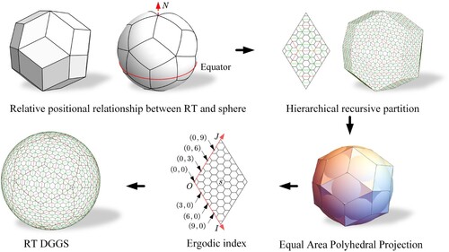
First, once a base polyhedron is selected, a fixed relative orientation between the RT and sphere must be specified. In this study, RT is oriented by placing two vertices at the north and south poles, allowing for more edges of the RT to be parallel to the longitudinal and latitudinal lines when mapping to the sphere. Second, the regular hierarchical grid is generated based on the subdivision of the aperture 4 hexagon on the polyhedral structure. Third, the equal-area mapping relationship is established based on the analysis of the geometric relationship between the RT and the sphere. Then, the polyhedral surface points correspond to the points on the spherical surface. Fourth, the corresponding transformation coordinate system is established on the rhombus structure according to the hierarchical division scheme of the grid.

A two-dimensional coordinate system and geometric distance were selected to illustrate the addresses of the surface. The rhombus face number was considered to be $s$, and the discrete grid coordinate $(i,j)$ ($i,j$ is a non-negative integer). Then, the center of a hexagonal cell in the rhombus was recorded, thereby helping cells assign a unique identifier and obtain the ergodic index of the grid. Finally, the equal-area projection was applied to obtain the RT DGGS. Moreover, the advantages of RT DGGS were evaluated by establishing grid evaluation indicators and performing efficiency tests.

3. Rhombic triacontahedron equal-area projection

The Snyder Equal-Area Polyhedral Projection is the most commonly used method for establishing platonic solid DGGS (Ben et al. 2006; Harrison, Mahdavi-Amiri, and Samavati 2011; Snyder 1992). Snyder Polyhedral Projection is usually applied to regular polygons. However, the rhombus surface of RT is not a regular polygon. Therefore, equal-area mapping between the RT and sphere must be performed. To accomplish this, a Rhombic Triacontahedron Equal-Area Mapping Projection (RTEA Projection) must be created to aid in the construction of the RT DGGS. The equal-area mapping process of forward projection from the local plane to the sphere and inverse projection from the sphere to the local plane can be established on a single rhombus face because of the symmetry of the RT and sphere. Then, the equal-area projection of the entire RT can be designed according to the symmetry.

3.1. Rhombic triacontahedron

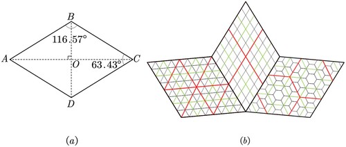
The RT (Weisstein 2022b) is a polyhedron comprising 30 golden rhombuses with 60 sides and 32 vertices. The obtuse angle of the rhombus is ${116.57}^{\circ }$ and its acute angle is ${63.43}^{\circ }$, unlike the platonic polyhedron that constructs the logical rhombus shape using the triangular surface, as shown in Figure 4(a). Therefore, the ability of the RT to produce the same equal-area cells by recursive division is unlike obtaining a regular polygon such as the platonic polyhedron (Figure 4(b)).

Figure 4. (a) Rhombic face of RT. (b) Rhombus recursive dissection produces equal-area cells of the same shape; from left to right are aperture 4 triangle, aperture 4 rhombus, and aperture 4 hexagon. Red represents the first level, green the second level, and black the third level.

Regular polygons (triangle, square, pentagon, hexagon) are applicable in Snyder Equal-Area Projection. However, there are no studies related to the rhombus, which is an axisymmetric polygon. When using Snyder Equal-Area Projection, the inscribed sphere and circumscribed sphere of platonic solids can be easily found, which allows for quickly achieving the transformation from vertex coordinates to the globe and determining the boundary of the local plane. Only the inscribed sphere of RT is identified, thus allowing for the determination of a suitable method to switch the points of the RT to the globe to realize the RTEA.

3.2. Forward projection

The equal-area condition of the RTEA can refer to Snyder Equal-Area Polyhedral Projection to project points on the earth to the RT. (1) The surface area of the RT and sphere equalize. (2) The area of a spherical triangle formed by a given azimuth remains unchanged after projection. (3) The point of the plane triangle can satisfy the differential condition of equal-area transformation.

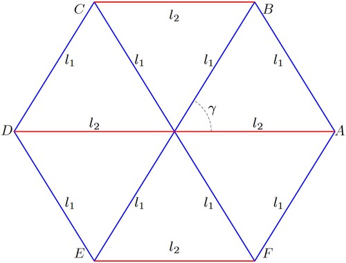
Only one right triangle needs to be considered because of the symmetry of the rhombus. As shown in Figure 5, the projection of the right angle spherical triangle $OAB$ is the plane right angle triangle $O^{\mathrm{\prime }}{A}^{\mathrm{\prime }}{B}^{\mathrm{\prime }}$. They have the same area. $O$ is the projection center. The length of the $OA$ edge is $\mathrm{g}$. The spherical angle between arc $OA$ and arc $AB$ is $G$. To deduce the corresponding relation within the basic unit, the projection of the azimuth $\alpha$ of arc $OE$ to plane right angle triangle $O^{\mathrm{\prime }}{A}^{\mathrm{\prime }}{B}^{\mathrm{\prime }}$ is $O^{\mathrm{\prime }}{E}^{\mathrm{\prime }}$ whose azimuth is $\delta$. Any point $T$ on the arc $OE$ is projected to be point $T^{\mathrm{\prime }}$ on $O^{\mathrm{\prime }}{E}^{\mathrm{\prime }}$. The arc lengths of $OT$ and $OE$ are $z$ and $q$, and the lengths of $O^{\mathrm{\prime }}{T}^{\mathrm{\prime }}$ and $O^{\mathrm{\prime }}{E}^{\mathrm{\prime }}$ are $\rho$ and $d$, respectively.

Figure 5. Corresponding relationship in basic unit.

Based on elementary geometry, the radius of the sphere is set as $R$, and the side length of the RT with the same area as the globe as $a$. The surface area of RT is $A_{polyhedron}=12\sqrt{5}{a}^2$; therefore, $a=\sqrt{\pi /\left(3\sqrt{5}\right)}R$. The radius of the inscribed sphere is $R^{\mathrm{\prime }}=\sqrt{1+1/\sqrt{5}}a$. Therefore, $A_{OAB}=A_{O^{\mathrm{\prime }}{A}^{\mathrm{\prime }}{B}^{\mathrm{\prime }}}=\pi R^2/30$, $G={36}^{\circ }$, and $\theta ={31.715}^{\circ }$ can be obtained from the geometric properties. Angle $H$, which is the spherical angle between arc $OE$ and arc $AB$, can be calculated using the spherical law of sines and cosines: (1) $H=\arccos (\sin \alpha \sin G\cos {\displaystyle \frac{g}{R}-\cos \alpha \cos G)}$(1) The area of the spherical triangle $OAE$ is expressed as follows: (2) $A_{OAE}=(\alpha +G+H-\pi )R^2$(2) By definition, $g/R$ is the spherical center angle corresponding to $g$, and $R^{\mathrm{\prime }}$ is its inscribed sphere radius, so according to $\tan \left(g/R\right)=(a\cdot \cos \theta )/R^{\mathrm{\prime }}$, (3) $g=R\cdot \arctan {\displaystyle \frac{a\cos \theta }{R^{\mathrm{\prime }}}}$(3) Furthermore, the area of plane triangle $O^{\mathrm{\prime }}{A}^{\mathrm{\prime }}{E}^{\mathrm{\prime }}$ is $A_{O^{\mathrm{\prime }}{A}^{\mathrm{\prime }}{E}^{\mathrm{\prime }}}=(O^{\mathrm{\prime }}{A}^{\mathrm{\prime }}\cdot O^{\mathrm{\prime }}{E}^{\mathrm{\prime }}\cdot \sin \delta )/2$, where $O^{\mathrm{\prime }}{A}^{\mathrm{\prime }}=R^{\mathrm{\prime }}\cdot tan\left(g/R\right)$; therefore, according to the law of sines, (4) $O^{\mathrm{\prime }}{E}^{\mathrm{\prime }}=O^{\mathrm{\prime }}{A}^{\mathrm{\prime }}{\displaystyle \frac{\sin \theta }{\sin (\pi -\delta -\theta )}={\displaystyle \frac{R^{\mathrm{\prime }}\sin \theta }{\sin (\theta +\delta )}\cdot \tan {\displaystyle \frac{g}{R}}}}$(4) Hence, the area of plane triangle $O^{\mathrm{\prime }}{A}^{\mathrm{\prime }}{E}^{\mathrm{\prime }}$ can be expressed as follows: (5) $A_{O^{\mathrm{\prime }}{A}^{\mathrm{\prime }}{E}^{\mathrm{\prime }}}={\displaystyle \frac{1}{2}(R^{\mathrm{\prime }}\tan {\displaystyle \frac{g}{R}{)}^2\cdot {\displaystyle \frac{\sin \theta \sin \delta }{\sin (\theta +\delta )}={\displaystyle \frac{1}{2}(R^{\mathrm{\prime }}\tan {\displaystyle \frac{g}{R}{)}^2{\displaystyle \frac{1}{\cot \theta +\cot \delta }}}}}}}$(5) Then, $\delta$ can be obtained according to equation (5)(5) $A_{O^{\mathrm{\prime }}{A}^{\mathrm{\prime }}{E}^{\mathrm{\prime }}}={\displaystyle \frac{1}{2}(R^{\mathrm{\prime }}\tan {\displaystyle \frac{g}{R}{)}^2\cdot {\displaystyle \frac{\sin \theta \sin \delta }{\sin (\theta +\delta )}={\displaystyle \frac{1}{2}(R^{\mathrm{\prime }}\tan {\displaystyle \frac{g}{R}{)}^2{\displaystyle \frac{1}{\cot \theta +\cot \delta }}}}}}}$(5) (6) $\delta =arccot({\displaystyle \frac{R^{\mathrm{\prime }2}{\tan }^2{\displaystyle \frac{g}{R}}}{2A_{OAE}}-\cot \theta )}$(6) To ensure that projection $A^{\mathrm{\prime }}{T}^{\mathrm{\prime }}$ of the large arc $AT$ on the triangle on the original sphere also satisfies the differential condition of the equal-area azimuth projection, $A^{\mathrm{\prime }}{T}^{\mathrm{\prime }}$ is scaled equally to $A^{\mathrm{\prime }\mathrm{\prime }}{T}^{\mathrm{\prime }\mathrm{\prime }}$, that is, (7) $\rho \cdot f=2R^{\mathrm{\prime }}\cdot \sin {\displaystyle \frac{z}{2R}}$(7) When $T^{\mathrm{\prime }}$ and $E^{\mathrm{\prime }}$, $T^{\mathrm{\prime }\mathrm{\prime }}$ and $E^{\mathrm{\prime }\mathrm{\prime }}$ coincide, the scaling factor can be calculated as follows: (8) $f={\displaystyle \frac{2R^{\mathrm{\prime }}\sin {\displaystyle \frac{q}{2R}}}{d}}$(8) Rewriting equation (7) using equation (8) yields the following equation: (9) $\rho ={\displaystyle \frac{\sin {\displaystyle \frac{z}{2R}}}{\sin {\displaystyle \frac{q}{2R}}}d}$(9) In the plane triangle $O^{\mathrm{\prime }}{A}^{\mathrm{\prime }}{E}^{\mathrm{\prime }\mathrm{\prime }}$, according to the law of sines: (10) ${\displaystyle \frac{O^{\mathrm{\prime }}{E}^{\mathrm{\prime }\mathrm{\prime }}}{\sin \theta }={\displaystyle \frac{O^{\mathrm{\prime }}{A}^{\mathrm{\prime }}}{\sin (\pi -\alpha -\theta )}}}$(10) Because $O^{\mathrm{\prime }}{E}^{\mathrm{\prime }\mathrm{\prime }}=R^{\mathrm{\prime }}\tan {\displaystyle \frac{q}{R}}$ and $O^{\mathrm{\prime }}{A}^{\mathrm{\prime }}=R^{\mathrm{\prime }}\tan {\displaystyle \frac{g}{R}}$, then. (11) $q=R\cdot \arctan ({\displaystyle \frac{\tan {\displaystyle \frac{g}{R}}}{\cos \alpha +\sin \alpha \cdot \cot \theta })}$(11) The projection radius $\rho$ can be obtained by substituting equations (4)(4) $O^{\mathrm{\prime }}{E}^{\mathrm{\prime }}=O^{\mathrm{\prime }}{A}^{\mathrm{\prime }}{\displaystyle \frac{\sin \theta }{\sin (\pi -\delta -\theta )}={\displaystyle \frac{R^{\mathrm{\prime }}\sin \theta }{\sin (\theta +\delta )}\cdot \tan {\displaystyle \frac{g}{R}}}}$(4) and (10)(10) ${\displaystyle \frac{O^{\mathrm{\prime }}{E}^{\mathrm{\prime }\mathrm{\prime }}}{\sin \theta }={\displaystyle \frac{O^{\mathrm{\prime }}{A}^{\mathrm{\prime }}}{\sin (\pi -\alpha -\theta )}}}$(10) into equation (9)(9) $\rho ={\displaystyle \frac{\sin {\displaystyle \frac{z}{2R}}}{\sin {\displaystyle \frac{q}{2R}}}d}$(9) ; therefore, the plane coordinates of $T^{\mathrm{\prime }}$ are as follows: (12) $\{\begin{array}{c}x=\rho \sin \delta \\ y=\rho \cos \delta \end{array}$(12)

3.3. Inverse projection

In the inversion process, the goal is to find the spherical coordinates of $T$ given the polyhedral coordinates of $T^{\mathrm{\prime }}$. Assuming point $T^{\mathrm{\prime }}$ of the polyhedron surface is $(x,y)$, the azimuth and projection radius can be obtained as follows: (13) $\{\begin{array}{c}\delta =\arctan \left(x/y\right)\\ \rho =\sqrt{x^2+y^2}\end{array}$(13) At the same time, the area of the spherical triangle $OAE$ can be obtained through point $T$. (14) $A_{OAE}={\displaystyle \frac{1}{2}\cdot (R^{\mathrm{\prime }}\tan {\displaystyle \frac{g}{R}{)}^2\cdot {\displaystyle \frac{1}{\cot \delta +\cot \theta }}}}$(14) Therefore, azimuth $\alpha$ is expressed as follows: (15) $\alpha ={\displaystyle \frac{A_{OAE}}{R^2}-G-H+\pi }$(15) Considering equation (15)(15) $\alpha ={\displaystyle \frac{A_{OAE}}{R^2}-G-H+\pi }$(15) as a nonlinear function for $\alpha$, then (16) $F\left(\alpha \right)={\displaystyle \frac{A_{OAE}}{R^2}-G-H-\alpha +\pi }$(16) Using Newton’s method to linearize the equation yields the following results: (17) $F^{\mathrm{\prime }}\left(\alpha \right)={\displaystyle \frac{\cos \alpha \cdot \sin G\cdot \cos \left(g/R^{\mathrm{\prime }}\right)+\sin \alpha \cdot \cos G}{\sin H}-1}$(17) (18) $\mathrm{\Delta }\alpha =-{\displaystyle \frac{F\left(\alpha \right)}{F^{\mathrm{\prime }}\left(\alpha \right)}}$(18) If ${\alpha }_0=\delta$, then $\alpha$ can be obtained by iterating the following equation. (19) ${\alpha }_{i+1}={\alpha }_i+\mathrm{\Delta }\alpha$(19) The final positioning of $T$ along arc $OT$ is simple using the proportionality from equation (7)(7) $\rho \cdot f=2R^{\mathrm{\prime }}\cdot \sin {\displaystyle \frac{z}{2R}}$(7) . (20) $z=2R\cdot \arcsin ({\displaystyle \frac{\rho f}{2R^{\mathrm{\prime }}})}$(20)

3.4. Implementation of projection

The derivation of the above equation is based on a basic unit as an example. This necessitates the use of the symmetry characteristics of the rhombus to convert a given point into the basic unit. Given the azimuth angle $\alpha$ and the given point $T$ in the first and third quadrants, the azimuth angle $\alpha$ can be adjusted directly according to the symmetry characteristics to ensure it falls within the interval $\left(0,\pi /2\right]$, and the adjusted angle $\mathrm{\Delta }w$ is recorded, as shown in Figure 6 (a). When the azimuth angle $\alpha$ of the given point $T$ is in the second and fourth quadrants, it is necessary to adjust the azimuth angle $\alpha$ according to $\left(n\pi \right)/2-\alpha n=1or3$. The azimuth angle $\alpha$ in the fourth quadrant $n=1$ and in the second quadrant $n=3$ helps it fall within the interval $\left(0,\pi /2\right]$, and the adjusted angle $\mathrm{\Delta }w$ needs to be recorded, as shown in Figure 6(b). Finally, the equal-area mapping of the rhombus can be realized using the equations derived by considering the basic unit as an example.

Figure 6. Transformation of the azimuth when the azimuth angle $\alpha$ of the given point $T$ is (a) in the first and third quadrants and (b) in the second and fourth quadrants.

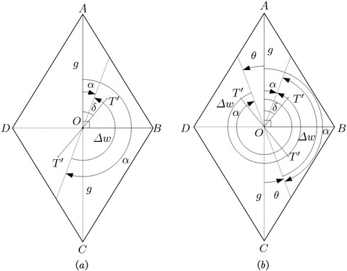
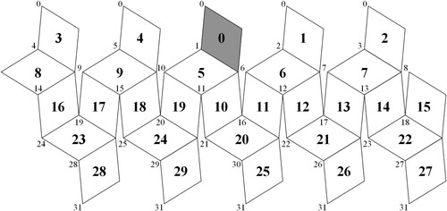
Owing to the projection carried out for each face, it is necessary to number each face of the RT after the single-rhombus surface algorithm is realized. Then, the longitudes and latitudes are easily determined for any given point and the sides of the RT mapped to the sphere can combine with the sphere. The setting rules are as follows (Figure 7): (1) the north and south poles are 0 and 31, (2) points 1, 11, and 21 are at the first meridian, and (3) the rest are analogized according to equal intervals to establish the face numbers of rhombuses.

Figure 7. RT expansion diagram and point distribution.

The points belonging to the sphere can be determined by constructing the unit vector of each side using Snyder Polyhedral Projection because platonic solids are equipped with a circumscribed sphere that helps the vertices of the platonic solid translate directly to the sphere. Because the RT has no circumscribed sphere, the translation of polyhedral vertices directly to the sphere cannot be realized as in platonic solids. According to the spatial geometric relationship analysis, the distance between the vertex of the RT and its geometric center satisfies the multiple of $1.107285080140779$ or $1.008286040002068$. Through these two parameters, the vertex of the spherical RT can be transformed into the corresponding vertex of the RT. Then, the rhombus to which one sphere point belongs can be determined by constructing the direction vector of RT on each side. The RTEA projection can be achieved through the above operations.

To simplify the calculation, the sphere radius was set to one. When the latitude and longitude of any point were $T(B,L)$, the calculation steps were as follows. According to the home plane number of $T(B,L)$, the longitude and latitude $O(B_0,L_0)$ of the projection center were obtained.

1. The spherical distance and azimuth of $OT$ were calculated according to the following equation. (21) $\{\begin{array}{c}z=\arccos [\sin B_0\sin B+\cos B_0\cos B\cos (L-L_0\left)\right]\\ \alpha =\arctan {\displaystyle \frac{\cos B\sin (L-L_0)}{\cos B_0\sin B-\sin B_0\cos B\cos (L-L_0)}}\end{array}$(21)

2. According to $\alpha$ and its position on the rhombus surface, the azimuth angle was adjusted to fall within the interval $(0,\pi /2)$, and the adjusted angle $\mathrm{\Delta }w$ was recorded.

3. $q$ was calculated according to equation (11)(11) $q=R\cdot \arctan ({\displaystyle \frac{\tan {\displaystyle \frac{g}{R}}}{\cos \alpha +\sin \alpha \cdot \cot \theta })}$(11) . If $z>q$, the distance between $T$ and $A$ was too long; therefore, its projection was supposed to be on the other faces of the polyhedron.

4. After adjusting the value of $\delta$ in step (2), the projection coordinate $T$ of $T^{\mathrm{\prime }}(x,y)$ could be calculated using equation (12)(12) $\{\begin{array}{c}x=\rho \sin \delta \\ y=\rho \cos \delta \end{array}$(12) .

The inverse calculation process is relatively simple and should be solved sequentially using the inverse transformation process equations. Based on the above discussion, the RTEA can be realized (Figure 8), thus forming the basis for the RT grid generation.

Figure 8. Equal-area projection of the RT.

4. Grid generation for the rhombic triacontahedron hexagonal discrete global grid system

The grid-generation algorithm is a fundamental step in the construction of a DGGS. We have established the corresponding equal-area projection between the sphere and the polyhedron surface employing RTEA forward and inverse projections. Upon identifying a specific partitioning method on a face or faces of the polyhedron, the mapping method can be used to create a similar topology relationship on spherical surfaces. There are always 12 pentagonal cells, regardless of the number of hexagonal cells. This is analogous to the DGGS based on icosahedron, which always has 12 pentagonal faces. In this study, cell affiliation was uncertain owing to the use of the hexagonal cell as the basic partitioning cell. Moreover, additional cases should be considered when constructing a DGGS because the RT has more faces than the icosahedron.

4.1. Construction of the coordinate system

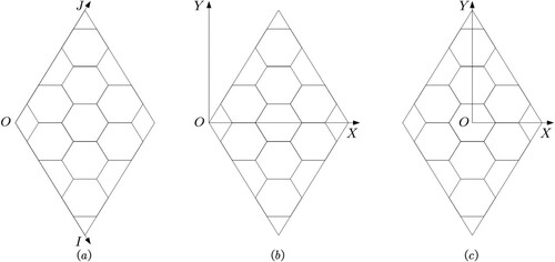
The goal of the grid-generation algorithm is to establish a unified mathematical model to describe the hexagonal rule coverage of 30 rhombus surfaces with specified partition levels and determine the spherical elements corresponding to the advanced support. According to Sahr, White, and Kimerling (2003), we denote the aperture 4 equal-area hexagonal grids based on RTEA as RTEA-H4 and establish three coordinate systems to describe the process of grid generation (Figure 9). The specific process functions are as follows:

1. The two-dimensional integer coordinate system is used to describe the grid cells that are regularly organized on the surface of RT. The angle between the axes is ${116.57}^{\circ }$. The parameters of the two-dimensional integer coordinate system are related to grid type and partition level. Supposing the recursion level of the grid is $n$; because the aperture 4 hexagonal grids are considered, the equal fraction of the rhomboid side length in the coordinates is $f=3\cdot 2^{n}n=0,1,2,3,\cdots ,$, and the values of grid coordinate parameters $I$ and $J$ are $0\le i,j\le f$. The two-dimensional integer coordinate system uniquely determines the central address through the above operation. The sequence number of the rhombus surface $s$ and the address of the grid center $(i,j)$ need to be recorded (Figure 9 (a)).

2. The transition coordinate system is used to establish a transformation between the two-dimensional integer coordinate system and plane Cartesian coordinate system, which is convenient for mapping the address to the sphere through RTEA (Figure 9 (b)).

3. The inverse equal-area projection coordinate system, for which the direction of the coordinate axis is consistent with that of RTEA, allows for the transformation between the plane point and the sphere (Figure 9 (c)). Spherical grids with different levels can be generated by adjusting the parameters of the above coordinate system according to actual needs upon completion of the construction of the above coordinate systems.

Figure 9. Illustration of the coordinate systems. (a) Two-dimensional integer coordinate system, (b) transition coordinate system, and (c) inverse equal-area projection coordinate system.

4.2. Arrangement of edge cells

In theory, the hexagonal cells on the common side of adjacent rhombuses belong to two different rhombuses. This leads to the non-unique attribution of the hexagonal cells, which is not conducive to the generation algorithm. Therefore, this study stipulates that the $J$-axis and corresponding edge elements in the two-dimensional integer coordinate system belong to the current rhombus (Figure 10). Pentagons are bound to appear on twelve vertices because the surface of the RT cannot be covered completely. Therefore, the hexagon at the vertex contains invalid parts, and the algorithm must first eliminate these and then splice the practical part of the common vertex into a complete pentagon.

Figure 10. Arrangement of edge hexagonal cells. $J$-axis and its corresponding edge cells in the two-dimensional integer coordinate system belong to the current rhombus delineated by the red lines in the figure.

4.3. Flow of grid generation

In the flow of grid generation, the adjacent hexagonal cells are staggered along the coordinate axis. The address of the hexagonal cells, $H[s,(i,j\left)\right]$, can be obtained through the two-dimensional integer coordinate system and the arrangement of edge cells (Figure 11(a)). The value range of the central coordinate of hexagonal cells is calculated according to the recursion level of the grid. The step size of direction $J$ is $\mathrm{\Delta }j=2$. Following an increase in the $I$ coordinate, the initial value $j_{{}_{inital}}$ of $J$ coordinate can be calculated using equation (22)(22) $j_{inital}=\{\begin{array}{c}0i\text{\%}3=0\\ 2i\text{\%}3=1\\ 1i\text{\%}3=2\end{array}$(22) . The index order is based on the above design, as shown in Figure 11(b). (22) $j_{inital}=\{\begin{array}{c}0i\text{\%}3=0\\ 2i\text{\%}3=1\\ 1i\text{\%}3=2\end{array}$(22) Considering the waist of the hexagonal grid cell $l_1$ and the bottom and top edges of the hexagonal cell $l_2$, the interior angle $\gamma$ required for calculation is ${58.285}^{\circ }$. As shown in Figure 12, edges with the same length are represented using the same color. Then, the coordinates of the central point $(i,j)$ in the transition coordinate system are presented as follows: (23) $\{\begin{array}{c}x=j\times l_2+(j-i)\times l_1\times \cos \gamma ,y=(j-i)\times l_1\times \sin \gamma i<j\\ x=i\times l_2,y=0i=j\\ x=j\times l_2+(i-j)\times l_1\times \cos \gamma ,y=(i-j)\times l_1\times \sin \gamma i>j\end{array}$(23) The calculation of the hexagonal cell boundary of the center point without considering the boundary condition is as follows. (24) $\{\begin{array}{c}{x}_A=x+2l_1\sin \gamma ,y_A=y\\ x_B=x+l_1\sin \gamma ,y_B=y+l_1\cos \gamma \\ x_C=x-l_1\sin \gamma ,y_C=y+l_1\cos \gamma \\ x_D=x-2l_1\sin \gamma ,y_D=y\\ x_E=x-l_1\sin \gamma ,y_E=y-l_1\cos \gamma \\ x_F=x+l_1\sin \gamma ,y_F=y-l_1\cos \gamma \end{array}$(24) The grid cells determine the attribution of the polygon vertex surface when the central point is located on the edge. Then, the corresponding hexagonal cells are generated according to the side length and angle of the hexagon. In addition, pentagonal cells are handled individually. In the final step, these grids are mapped to the sphere through the transition coordinate system and inverse equal product mapping coordinate system, as shown in Figures 11 (c) and (d), and finally to the sphere with the help of RTEA.

Figure 11. RTEA-H4 coordinate transformation. (a) The points in the two-dimensional integer coordinate system, (b) retrieval order of points, (c) conversion to transition coordinate system, and (d) conversion to inverse equal-area projection coordinate system.

Figure 12. A hexagonal cell. The same color represents the same length of edges: blue represents $l_1$, and red represents $l_2$. The angle required for the calculation of hexagonal cells from the discrete grid coordinate system to the excessive coordinate system is $\gamma$.

5. Design of experiments

RT DGGS can be constructed through the analysis of the above algorithms. We designed the following experiments to verify the advantages of the model.

Experiment 1: Grid generation. To verify the feasibility of the model, we generated the grid for the RT hexagonal DGGS. We adopted the equal-area radius of the WGS-84 reference ellipsoid as the spherical radius to ensure that the spherical grid maintained the equal-area property when expanding to the ellipsoid. Consequently, the side length of the RT was $4359933.90316m$. The hexagonal grid on the surface of the RT was transformed into the sphere by the RTEA inverse projection. First, the number of the grid level was determined and a planar hexagonal grid was constructed on the surface of the RT according to the aperture 4 hexagon scheme. Second, the pentagonal cells were addressed separately during the construction process, the index order of the planar hexagon was determined, and the grid boundary was generated. For the hexagon located on the edge, the number of faces on the boundary point should be determined. Finally, the planar grid was mapped to the sphere with the help of RTEA and the result was outputted (Figure 13). During grid generation, the number and area of cells in the level were recorded and compared with a similar area of the icosahedral DGGS method, which uses Icosahedral Snyder Equal-Area Projection (ISEA Projection).

Figure 13. Process of generating the spherical RT hexagonal grid.

Experiment 2: Comparison of grid characteristics. To verify the advantages of our method over traditional icosahedral methods that used ISEA, we evaluated the angular distortion and shape of cells.

The angle distortion is only considered when evaluating the mapping relationship because both methods are based on equal-area projection. In this study, referring to Tissot’s theorem, an infinitesimal circle on a sphere was projected onto the plane to generate an ellipse (van Leeuwen and Strebe 2006) (Figure 14).

Figure 14. Angle distortion on the RT.

Assuming the major axis of the error ellipse to be $a$ and its minor axis $b$, the angle distortion of the mapping $w$, was calculated using equation (25)(25) $w=2\times \arcsin {\displaystyle \frac{a-b}{a+b}}$(25) . The angle distortion of the projection can be represented by a single face because both the icosahedron and RT are symmetrical. We designed numbers of longitude and latitude points uniformly selected in a single plane of the spherical icosahedron and the spherical RT. Infinitesimal circles were generated according to these points, and projected onto the icosahedral and RT surfaces. Using $w$ in equation (25)(25) $w=2\times \arcsin {\displaystyle \frac{a-b}{a+b}}$(25) provides an estimate of the distortion at all the sampled circle centers. Icosahedron and RT obtained the mean and standard deviation of the angle distortion by calculating the angle distortion values of all the circles. (25) $w=2\times \arcsin {\displaystyle \frac{a-b}{a+b}}$(25) Regardless of platonic solids and RT, owing to the geometric properties of the sphere, only elements with approximately the same index can be obtained. Therefore, we constructed quantifiable grid evaluation indexes to analyze the geometric properties of cells when the cell sizes for all methods are similar under the aperture 4 hexagon.

For the shape measurement of grid cells, we used compactness to evaluate the DGGS grid shape (Kimerling et al. 1999; White et al. 1998) using the formula $\sqrt{(4\pi a-a^2/r^2)}/p$, where $a$ is the area of the grid cell, $p$ is the perimeter of the grid cell, and $r$ is the sphere radius. The compactness of each hexagonal cell was calculated, the average of all cells was selected as a representation of the compactness of the corresponding level, and the standard deviation at that level was recorded.

The difference in grid edge length is one of the essential indicators for measuring grid consistency (Sun and Zhou 2016). Therefore, the length deviation rate was introduced to analyze the deformation of the grid edge. The rate of length deviation can be expressed as $P_L=(L_N-L)/L$, where $P_L$ is the length deviation rate, $L$ is the side length of the plane grid before projection, and $L_N$ is the projected grid side length. When utilizing the two methods to measure the grid length deviation, we calculated the length deviation of each side of the hexagon and considered the maximum value as the length deviation of the cell. The average of all hexagonal cells was designated as the length deviation of the corresponding level and denoted as the standard deviation of the length deviation of the level.

The difference in angle is one of the important indexes for measuring the uniformity of the grid (Sun and Zhou 2016). Similar to the length deviation, the angle deviation rate is used to measure the deformation of the angle. The rate of angular deviation can be expressed as $P_A=(A_N-A)/A$, where $P_A$ is the rate of angular deviation, where $A$ is the angle of the plane grid before the projection and $A_N$ is the angle of the grid after the projection. We considered the maximum as the angle deviation of the grid cells by calculating the angle value of the six inner angles of the spherical hexagon and the angle value of the corresponding plane hexagon. We also calculated the mean of all hexagonal cells as the angle deviation of the current level and recorded the standard deviation.

We used six statistics of three types of measurements: the mean and the standard deviation of compactness, the mean and the standard deviation of length deviation, and the mean and the standard deviation of angle deviation. We discuss the different indexes and analyze the geometric properties of the two methods.

Experiment 3: Coding operation efficiency test. An increase in the surface will affect the efficiency of the cross-surface calculation and the calculation efficiency of the entire global discrete grid system. Therefore, we designed comparative experiments to verify the effect of the increase in the RT DGGS surface on efficiency.

The comparative experiments focused on the basic encoding operations of icosahedral DGGS and RT DGGS: (1) the conversion of latitude and longitude into codes, (2) the conversion of codes into latitude and longitude, and (3) neighborhood query. Through the global traversal of the latitude and longitude coordinates, the step size was set to 0.2 degrees, and we obtained 1.62 million points as test data.

In the experiments, we first converted the longitude and latitude to codes. Next, the codes were converted to longitude and latitude and we obtained their neighborhood codes and recorded the total time consumed by each simultaneously. Finally, we calculated the efficiency ratio of the two methods. All experiments were implemented using Microsoft Visual Studio on Windows 10 x64 platform Enterprise 2022 Visual C++ Release version, with six Intel(R) Core(TM) i5-9500F CPUs @ 3.00 GHz.

6. Results and analysis

6.1. Grid generation

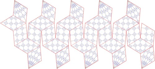
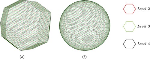
According to the experimental design, the aperture 4 Hexagon DGGS on both the RT and sphere is successfully generated through the above experimental designing, which proves the algorithm’s feasibility and aids in the analysis of the advantages of the RT DGGS. The program generated the aperture 4 hexagonal grid on the surface of the RT and sphere, and the resolutions were 2, 3, and 4 (Figure 15).

Figure 15. RTEA-H4 DGGS. Hexagonal grid on the surface of the (a) RT and (b) sphere. The RTEA-H4 DGGSs’ levels are 2, 3, and 4: the level 2 hexagonal color is red, level 3 is green, and level 4 is black.

We recorded the performance of two methods with respect to the number of cells and cell area. The number of hexagonal cells in the grid of the two methods increased exponentially as the resolutions increased. The RT DGGS exhibits relatively high resolution and segmentation efficiency at the same level. When the sizes of the cells of the two methods were similar, the cell area in the RT DGGS was relatively large, and the cell number was less than that in the icosahedral method Table 1.

Table 1. Number of cells and cell areas in DGGSs based on the spherical icosahedron and RT.

Level	Number of cells (Icosahedron)	Cell area (Icosahedron) km^2	Number of cells (RT)	Cell area (RT) km^2
1	32	17,002,187.616	80	5,667,395.873
2	122	4,250,546.904	350	1,416,848.968
3	482	1,062,636.726	1,430	354,212.000
4	1,922	265,659.182	5,750	88,553.100
5	7,682	66,414.795	23,030	22,138.300
6	30,722	16,603.699	92,150	5,534.570
7	122,882	4,150.925	368,630	1,383.64
8	491,522	1,037.731	1,474,550	345.91
9	1,966,082	259.433	5,898,230	86.478
10	7,864,322	64.585	23,592,950	21.620

6.2. Comparison of grid characteristics

6.2.1. Angle distortion

As shown in Table 2, the mean and standard deviation of the RTEA angle distortion decreased by approximately 41.6% and 30.9%, respectively, compared with those of the ISEA projection. The angle distortion of the RT method was reduced significantly. Therefore, small angle distortion of the grid generation according to RTEA is more conducive to the modeling and management of geospatial data.

Table 2. Comparison of error conditions.

	Mean	Standard deviation
Icosahedron	0.166	0.055
Rhombic Triacontahedron	0.097	0.038

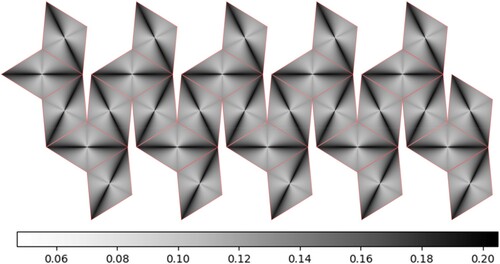
The error can be displayed on rhombic and triangular surfaces using grayscale to visualize the angular distortion, with black representing large distortion and white representing minor distortion. The smaller the distortion, the brighter is the color of the section. Figure 16 shows that RT distortion was mainly concentrated along the direction of the long axis of the rhombus. The icosahedral distortion was concentrated along the direction from the center point of the face to the three vertices. The overall color of the rhombus was lighter than that of the triangle. Moreover, the angular distortion of the RT was smaller than that of the icosahedron.

Figure 16. Distribution of angular distortion. Angular distortion is demonstrated on the face of (a) an icosahedron and (b) an RT through the grayscale values.

For further analysis, we determined the angular distortion $w$ of each face of the RT and expanded it as shown in Figure 7, thereby obtaining the entire deformation of the RTEA. As shown in Figure 17, the overall angular distortion is consistent with the angular distortion of a single face. The distortion was relatively large in the long axis direction, and the color in this direction was darker than that in the other areas. The angular distortion on both sides of the short axis is relatively small on the face. Furthermore, the axisymmetric characteristics are demonstrated by the relatively bright color, and the smallest angular deformation is observed at the center of the rhombic surface.

Figure 17. Angle distortion of RTEA.

Based on the above experiment, a significant improvement of the RTEA can be based on the following reasons: (1) Compared with the icosahedron, the RT has more faces, and its shape is closer to that of a sphere. (2) The projections of both methods are reference equal-area azimuthal projections. Both methods use the center of the surface as the projection point, and the angular deformation radiates outward from the center of the surface. The area of a single face of the RT is smaller than that of the icosahedron, resulting in a reduced angular distortion of the RTEA. The experimental results show that RT outperforms the icosahedron in constructing DGGS.

6.2.2. Geometric properties of the grids

To compare the geometric properties of the grids, the cell sizes of the two methods were made similar. Only hexagonal cells were considered in the comparison. Upon the calculation and recording of the deformation index of each level (Table 3), the following characteristics were obtained.

1. Compactness. The mean and standard deviation of compactness for the two methods were calculated and are presented in Table 3. Figure 18 shows the two indicators gradually stabilized as the level increased. The higher the values of the average compactness, the closer they were to the most compact shape possible. Furthermore, the standard deviation of compactness was smaller by 39.6% than that in the traditional method. The experimental results showed that the performance of the RT method was more optimized than that of the icosahedron. The overall shape of the spherical hexagonal grid cell based on RT was more stable and regular than that based on the icosahedron, and this was beneficial to the establishment of the hexagonal DGGS.

2. Length deviation. The results of each level are shown in Table 3. Figure 19 shows that as the subdivision level increases, the mean and standard deviation of the length deviation tend to be less pronounced, and the mean and standard deviation of the grid length deviation of icosahedron were 0.0577 and 0.0204, respectively. The mean and standard deviation of the length deviation of RT were 0.0323 and 0.0137, respectively. The mean and standard deviation of the length deviation of RT decreased by 44% and 32.8% compared to those of the icosahedron, respectively.

Figure 18. Comparison of the compactness measurement of the two methods. (a) The mean of compactness and (b) the standard deviation of compactness.

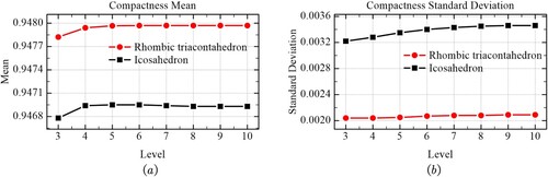
Figure 19. Comparison of length deviation measurements of the two methods. (a) Mean of the length deviation. (b) Standard deviation of the length deviation.

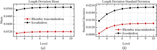
Table 3. Geometric properties of grids for aperture 4 hexagons on the spherical icosahedron and RT.

	Level	Compactness		Length deviation		Angle deviation
		Mean	Standard deviation	Mean	Standard deviation	Mean	Standard deviation
Icosahedron	3	0.94679	0.00322	0.05466	0.01477	0.04437	0.01211
	4	0.94694	0.00328	0.05623	0.01750	0.04712	0.01463
	5	0.94695	0.00335	0.05700	0.01897	0.04861	0.01620
	6	0.94695	0.00340	0.05737	0.01970	0.04940	0.01708
	7	0.94694	0.00343	0.05755	0.02005	0.04980	0.01755
	8	0.94693	0.00345	0.05763	0.02022	0.05001	0.01779
	9	0.94693	0.00346	0.05768	0.02031	0.05012	0.01791
	10	0.94693	0.00346	0.05770	0.02035	0.05017	0.01798
Rhombic triacontahedron	3	0.94782	0.00206	0.03043	0.00969	0.03221	0.00838
	4	0.94794	0.00204	0.03141	0.01173	0.03369	0.01037
	5	0.94797	0.00205	0.03186	0.01280	0.03453	0.01178
	6	0.94797	0.00207	0.03207	0.01329	0.03502	0.01259
	7	0.94797	0.00208	0.03217	0.01351	0.03530	0.01303
	8	0.94797	0.00208	0.03222	0.01360	0.03544	0.01326
	9	0.94797	0.00209	0.03224	0.01365	0.03552	0.01338
	10	0.94797	0.00209	0.03225	0.01367	0.03556	0.01344

To further analyze the length deviation, we reference the energy quantization of angular distortion $w$ considering the single surface of the RT and icosahedron as the example, quantifying the value of the length deviation of each grid cell in level 7. At this point, the $P_{Lmax}$ and $P_{Lmin}$ of the RT were 0.0656722 and 0.0157911, and those of the icosahedron $P_{Lmax}$ and $P_{Lmin}$ were 0.101339 and 0.0232165.

As shown in Figure 20, the dark colored section indicates that the length deviation is relatively large and the light colored section indicates that the deviation rate is relatively low. Their variations are consistent with the projection characteristics. This means that the length deviation of the cell depends on the equal-area projection. The RT has less angle distortion than the icosahedron. Therefore, the brightness distribution was similar to the angular distortion and RT exhibited a relatively light color, indicating that the length deviation of the RT was smaller than that of the icosahedron.

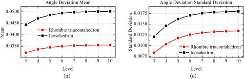
(3)

Angle deviation. The average angle deviation rate and standard deviation of each grid level are shown in Table 3. As shown in Figure 21, as the subdivision level increases, the mean and standard deviation of the angle deviation rate of the cells gradually decrease. The mean and standard deviation of the angle deviation of icosahedral cells approached 0.0502 and 0.0180, respectively. The mean and standard deviation of the length deviation of the RT method approached 0.0356 and 0.0134, respectively. The mean and standard deviation of the angle deviation of the RT cells decreased by approximately 29.1% and 25.6% compared with those of the icosahedral cells.

Figure 20. Distribution of length deviation. Length deviation shown at a face of (a) an icosahedron and (b) an RT through grayscale values.

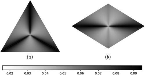
Figure 21. Comparison of the angular deviation measurement of the two methods. (a) Mean of angular deviation and (b) angular deviation of length deviation.

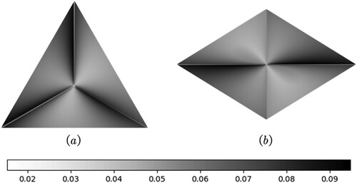
The rate of angular deviation can be quantified on a single face of the icosahedron and RT. Similarly, the angle deviation of each grid cell in level 7 can be quantified. The $P_{Amax}$ and $P_{Amin}$ of RT were 0.075764 and 0.023928, and the $P_{Amax}$ and $P_{Amin}$ of the icosahedron were 0.0976778 and 0.01572725, respectively. Owing to the characteristics of the equal-area projection of the two methods, the error direction of the triangular surface is larger than that of the rhombic surface. Furthermore, according to the connection line, the aperture 4 hexagon is perpendicular to the edge of the rhombus structure in this study. We also found that the distribution of the hexagon on the triangular surface will cause the angle error to be larger than that of the RT. As shown in Figure 22, the overall tone of the RT was brighter than that of the icosahedron (Figure 22).

Figure 22. Distribution of angle deviation. Angle deviation is shown on the face of (a) an icosahedron through the grayscale value and (b) an RT through grayscale values.

A comparison of grid characteristics showed that the angle distortion of the RT is smaller and the geometric properties of the RT’s grid were better than those of the icosahedron grid. The RT DGGS characteristics exhibited better properties than the icosahedron DGGS.

6.3. Coding operation efficiency test

To ensure objectivity and fairness of the experiments, all functions were run ten times, and the average time taken was used as the time taken for each operation. The experimental data obtained are shown in Table 4.

Table 4. Results of comparison of experimental efficiency.

Level	Latitude and longitude converting to codes			Codes converting to latitude and longitude			Neighborhood query
	Icosahedron ($\mu s$ )	Rhombic Triacontahedron ($\mu s$)	Efficiency ratio	Icosahedron ($\mu s$)	Rhombic Triacontahedron ($\mu s$)	Efficiency ratio	Icosahedron ($\mu s$)	Rhombic Triacontahedron ($\mu s$)	Efficiency ratio
11	0.000518	0.000536	0.967577	0.000638	0.000618	1.032309	0.000810	0.000446	1.813822
12	0.000536	0.000552	0.970909	0.000651	0.000629	1.034407	0.001483	0.000788	1.881776
13	0.000545	0.000561	0.972747	0.000653	0.000631	1.034791	0.002789	0.001437	1.940314
14	0.000556	0.000571	0.973660	0.000658	0.000635	1.036096	0.005455	0.002743	1.988966
15	0.000562	0.000577	0.975340	0.000669	0.000645	1.037209	0.010622	0.005322	1.995951
16	0.000575	0.000588	0.977550	0.000672	0.000647	1.038022	0.021124	0.010512	2.009416
17	0.000584	0.000596	0.979255	0.000676	0.000650	1.039741	0.042017	0.020845	2.015721
18	0.000596	0.000607	0.980617	0.000680	0.000654	1.040189	0.083706	0.041487	2.017632
19	0.000606	0.000617	0.980951	0.000685	0.000658	1.041915	0.167072	0.082737	2.019314
20	0.000617	0.000628	0.981982	0.000692	0.000663	1.042928	0.334540	0.165579	2.020424

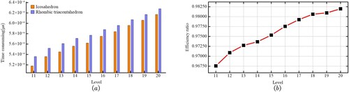
Conversion of latitude and longitude to codes. Compared with the icosahedron DGGS, the RT DGGS proposed in this study is more complicated to judge the cross-plane attribution of the encoding. Encoding latitude and longitude under the RT DGGS framework is not as fast as that in the icosahedral DGGS. However, with the increase in subdivision levels, the efficiency of the RT will gradually increase (Figure 23). The advantages of RT are then reflected. A set of adjacent edges on its rhombus face is a natural two-dimensional coordinate system, which easily describes the cell location. Further, the cells’ code of RT does not require judging of the triangle again when coordinating transformation conversion as with the icosahedron.

Figure 23. Efficiency comparison for latitude and longitude converting to codes. (a) Comparison of the time consumed by the two schemes. (b) Efficiency ratio of the two schemes.

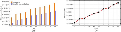
Comparison of the efficiency of code conversion to latitude and longitude. In this operation, the code first converts to $(x,y)$ of the polyhedron surface. Then, it maps to the spherical surface through the equal-area coordinates. Finally, the geographic coordinates are obtained. The icosahedron can use two triangular faces to form a ‘rhombus’ as the basic structure for division and coding. However, it is not an ideal rhombus structure. Specifically, the two triangular faces are not located in the same plane, which increases the cell position description and the difficulty of increasing the complexity of grid-related operations. In the operation, the cell encoding of the icosahedral DGGS must perform many triangular and logical rhombus judgments. The rhombus, as the basic unit of RT, directly converts the plane coordinates $(x,y)$ to latitude and longitude. Its structure greatly reduces the repeated calculation and improves efficiency. Therefore, the RT's efficiency is greater than that of the icosahedron, as shown in Figure 24.

Figure 24. Comparison of the efficiency of encoding conversion to latitude and longitude. (a) Comparison of the time consumed by the two schemes. (b) Efficiency ratio of the two schemes.

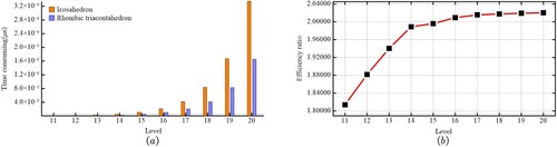
Neighborhood query. The hexagon has six adjacent cells with sides in different directions. Therefore, further judgment is required when querying adjacent units when they are across. When using encoding for querying, RT is less complicated than the icosahedron because of its symmetry. It can divide the types of edge cells similar to the icosahedron. However, the neighborhood query average efficiency of RT is approximately twice that of the icosahedron (Table 4). Furthermore, its efficiency ratio increases gradually with the level (Figure 25). Because both schemes rely on coded addition operations, the efficiency of coding operations decreases as the level increases (Figure 25(b)).

Figure 25. Neighborhood query efficiency comparison. (a) Comparison of the time consumed by the two schemes. (b) Efficiency ratio of the two schemes.

7. Conclusion

This paper proposed a new DGGS construction method based on RT. Further, this study established the RTEA projection and constructed the hexagonal RT DGGS according to the characteristics of the aperture 4 hexagon subdivision, which expands the definition of DGGS and benefits the study of Catalan polyhedral DGGS, for example, rhombic dodecahedron.

Compared with the traditional icosahedron DGGS, the method proposed in this study exhibited noticeable improvement in both angle distortion of projection and geometric properties of the grid cells. It is more suitable for hexagonal grid modeling and provides a remarkable model basis for geospatial data processing and analysis, thus exhibiting application potential. Furthermore, as the surface increases, the efficiency of RT's cross-surface calculations is not significantly reduced, and it has more advantages in encoding the conversion to latitude and longitude and proximity queries. In future research, we will continue to focus on the research method based on hexagonal RT DGGS and adopt a more efficient coding index operation to provide theoretical and technical support to help solve the problem of large-scale spatial data organization.

Data availability

Data sharing not applicable to this article as no datasets were generated or analysed during the current study.

Disclosure statement

No potential conflict of interest was reported by the author(s).

Additional information

Funding

This work was supported by the Special Science Fund for Innovation Ecosystem Construction of National Supercomputing Center in Zhengzhou [grant no 201400210100] and the National Key Research and Development Program of China [grant no 2018YFB0505301].

References

- Ben, J., Y. Li, C. Zhou, R. Wang, and L. Du. 2018. “Algebraic Encoding Scheme for Aperture 3 Hexagonal Discrete Global Grid System.” Science China Earth Sciences 61 (2): 215–227. doi:10.1007/s11430-017-9111-y.
- Ben, J., X. Tong, Y. Zhang, and H. Zhang. 2006. “Snyder Equal-Area Map Projection for Polyhedral Globes.” Geomatics and Information Science of Wuhan University 31 (10): 900–903.
- Bowater, D., and E. Stefanakis. 2019. “On the Isolatitude Property of the RHEALPix Discrete Global Grid System.” Big Earth Data 3 (4): 362–377. doi:10.1080/20964471.2019.1658494.
- Goodchild, M. F., H. Guo, A. Annoni, L. Bian, K. De Bie, F. Campbell, M. Craglia, et al. 2012. “Next-Generation Digital Earth.” Proceedings of the National Academy of Sciences 109 (28): 11088–11094. doi:10.1073/pnas.1202383109.
- Han, B., T. Qu, Z. Huang, Q. Wang, and X. Pan. 2021. “Emergency Airport Site Selection Using Global Subdivision Grids.” Big Earth Data, 1–18. doi:10.1080/20964471.2021.1996866.
- Harrison, E., A. Mahdavi-Amiri, and F. Samavati. 2011. “Optimization of Inverse Snyder Polyhedral Projection.” In 2011, International Conference on Cyberworlds, 136–143. doi:10.1109/CW.2011.36.
- Hojati, M., C. Robertson, S. Roberts, and C. Chaudhuri. 2022. “GIScience Research Challenges for Realizing Discrete Global Grid Systems as a Digital Earth.” Big Earth Data, 1–22. doi:10.1080/20964471.2021.2012912.
- Kimerling, J. A., K. Sahr, D. White, and L. Song. 1999. “Comparing Geometrical Properties of Global Grids.” Cartography and Geographic Information Science 26 (4): 271–288. doi:10.1559/152304099782294186.
- Peterson, P. 2011. “Close-Packed Uniformly Adjacent, Multiresolutional Overlapping Spatial Data Ordering.” US Patent 8,018,458, filed September 13.
- Peterson, P. R. 2016. “Discrete Global Grid Systems.” International Encyclopedia of Geography: People, the Earth, Environment and Technology 2016: 1–10. doi:10.1002/9781118786352.wbieg1050.
- Qu, T., L. Wang, J. Yu, J. Yan, G. Xu, M. Li, C. Cheng, K. Hou, and B. Chen. 2020. “STGI: a Spatio-Temporal Grid Index Model for Marine big Data.” Big Earth Data 4 (4): 435–450. doi:10.1080/20964471.2020.1844933.
- Rawson, A., Z. Sabeur, and M. Brito. 2021. “Intelligent Geospatial Maritime Risk Analytics Using the Discrete Global Grid System.” Big Earth Data, 1–29. doi:10.1080/20964471.2021.1965370.
- Sahr, K. 2008. “Location Coding on Icosahedral Aperture 3 Hexagon Discrete Global Grids.” Computers, Environment and Urban Systems 32 (3): 174–187. doi:10.1016/j.compenvurbsys.2007.11.005.
- Sahr, K., D. White, and A. J. Kimerling. 2003. “Geodesic Discrete Global Grid Systems.” Cartography and Geographic Information Science 30 (2): 121–134. doi:10.1559/152304003100011090.
- Snyder, J. P. 1992. “An Equal-Area Map Projection For Polyhedral Globes.” Cartographica: The International Journal for Geographic Information and Geovisualization 29 (1): 10–21. doi:10.3138/27H7-8K88-4882-1752.
- Suess, M., P. Matos, A. Gutierrez, M. Zundo, and M. Martin-Neira. 2004. “Processing of SMOS Level 1c Data Onto a Discrete Global Grid.” IEEE International Geoscience and Remote Sensing Symposium 3: 1914–1917. doi:10.1109/IGARSS.2004.1370716.
- Sun, W., and C. Zhou. 2016. “Distortion Analysis of Approximate Equal-Area Grids Based on Octahedron.” Geomatics and Information Science of Wuhan University 41 (12): 1577–1583. doi:10.13203/j.whugis20140844.
- Tang, X., X. Yao, D. Liu, L. Zhao, L. Li, D. Zhu, and G. Li. 2021. “A Ceph-Based Storage Strategy for Big Gridded Remote Sensing Data.” Big Earth Data, 323–339. doi:10.1080/20964471.2021.1989792.
- Thompson, J. A., M. J. Brodzik, K. A. Silverstein, M. A. Hurley, and N. L. Carlson. 2022. “EASE-DGGS: A Hybrid Discrete Global Grid System for Earth Sciences.” Big Earth Data, 340–357. doi:10.1080/20964471.2021.2017539.
- van Leeuwen, D., and D. Strebe. 2006. “A "Slice-and-Dice" Approach to Area Equivalence in Polyhedral Map Projections.” Cartography and Geographic Information Science 33 (4): 269–286. doi:10.1559/152304006779500687.
- Wang, R., J. Ben, J. Zhou, and M. Zheng. 2020. “Indexing Mixed Aperture Icosahedral Hexagonal Discrete Global Grid Systems.” ISPRS International Journal of Geo-Information 9 (3): 171. doi:10.3390/ijgi9030171.
- Wang, R., J. Ben, J. Zhou, and M. Zheng. 2021. “A Generic Encoding and Operation Scheme for Mixed Aperture Three and Four Hexagonal Discrete Global Grid Systems.” International Journal of Geographical Information Science 35 (3): 513–555. doi:10.1080/13658816.2020.1763363.
- Weisstein, Eric. W. 2022a. “Catalan Solid.” From MathWorld–A Wolfram Web Resource. https://mathworld.wolfram.com/CatalanSolid.html.
- Weisstein, Eric. W. 2022b. “Rhombic Triacontahedron.” From MathWorld–A Wolfram Web Resource. https://mathworld.wolfram.com/RhombicTriacontahedron.html.
- White, D., A. J. Kimerling, K. Sahr, and L. Song. 1998. “Comparing Area and Shape Distortion on Polyhedral-Based Recursive Partitions of the Sphere.” International Journal of Geographical Information Science 12 (8): 805–827. doi:10.1080/136588198241518.
- Yao, X., G. Li, J. Xia, J. Ben, Q. Cao, L. Zhao, Y. Ma, L. Zhang, and D. Zhu. 2019. “Enabling the Big Earth Observation Data via Cloud Computing and DGGS: Opportunities and Challenges.” Remote Sensing 12 (1): 62. doi:10.3390/RS12010062.
- Zhao, X., J. Ben, W. Sun, and X. Tong. 2016. “Overview of the Research Progress in the Earth Tessellation Grid.” Acta Geodaetica et Cartographica Sinica 45: 1–14. doi:10.11947/j.AGCS.2016.F001.
- Zhou, J., J. Ben, R. Wang, M. Zheng, and L. Du. 2020a. “Lattice Quad-Tree Indexing Algorithm for a Hexagonal Discrete Global Grid System.” ISPRS International Journal of Geo-Information 9 (2): 83. doi:10.3390/ijgi9020083.
- Zhou, J., J. Ben, R. Wang, M. Zheng, X. Yao, and L. Du. 2020b. “A Novel Method of Determining the Optimal Polyhedral Orientation for Discrete Global Grid Systems Applicable to Regional-Scale Areas of Interest.” International Journal of Digital Earth 13 (12): 1553–1569. doi:10.1080/17538947.2020.1748127.